Annual Evaluation of Natural Ventilation Induction in Solar Chimneys under Tropical, Dry, and Temperate Climates of Mexico: A Case Study ^†

Abstract

This article presents an annual performance evaluation of single- and double-air-channel solar chimneys for natural ventilation induction under weather conditions in Mexico. The global energy balance method modeled both types of solar chimneys in an unsteady state. The case study evaluated five cities in Mexico. Experimental data of a single-air-channel chimney prototype evaluated under controlled conditions were used to validate the GEB numerical solution. Model validation considers climatic parameters to increase the accuracy of ventilation calculations, e.g., solar radiation, ambient temperature, wind speed, relative humidity, and atmospheric pressure. Experimental evaluation was performed considering the warmest and coldest days in each month of 2018. The modeling time to achieve the initial condition independence for each configuration was 72 h of the physical phenomenon. Results show that double-air-channel solar chimney tested configurations induced at least 70% more airflow than single-air-channel solar chimneys. Both solar chimney airflows were higher than the dwelling-unit ventilation for a space of 54 m${}^3$, and volumetric flows up to 120 m${}^3$h${}^{-1}$ were identified for two studied cities.

1. Introduction

The process of replacing stale air with fresh air is ventilation. In buildings, ventilation removes stagnant air from indoor spaces to moderate contaminants, humidity, and even temperature levels impacting indoor air quality (IAQ) [1]. IAQ impacts building occupants’ health, welfare, and comfort, e.g., the emergence of the COVID-19 pandemic [2,3,4,5]. This way, ventilation is crucial where people spend up to 90% of their time, e.g., households, factories, offices, recreational areas, and establishments [6,7]. However, mainly in old buildings, building design does not support supplying air to and removing air from indoor spaces to induce natural ventilation. Thus, residents use mechanical systems, e.g., active systems such as air conditioners and fans, generating considerable energy consumption. According to the International Energy Agency (IEA) [8], 36% of global energy consumption was by the residential and construction sector, where 30% of the energy consumed in buildings was dissipated through ventilation and exfiltration systems before the COVID-19 pandemic [9]. In 2021, the energy efficiency report of the IEA stated that the new orientation towards building managers suggests increasing the ventilation rate to reduce the transmission of COVID-19 [10]. The IEA projections suggest that increasing the ventilation rate through active systems represents an increase of 10% in total energy consumption for non-residential buildings. Therefore, it is necessary to address the natural ventilation problem by providing alternative ventilation mechanisms in buildings without exceeding the energy consumption that represents an excessive consumption of natural resources.

In Mexico, the Energy Ministry reports that 25.9% of total electricity consumption corresponds to the residential sector [11]. This is a direct consequence of using active systems, i.e., refrigeration and air conditioning devices. According to statistics from the National Institute of Statistics and Geography (INEGI), 45% of households have mechanical ventilation systems, and just over 20% have air conditioning [12]. The current energy scenario in Mexico requires alternatives to satisfy the demand for ventilation through unconventional methods, such as using renewable energy. Among the alternatives is using passive systems, e.g., solar chimneys. A solar chimney is a device attached to the room’s roof or façade that works through solar energy to induce air renewal in the housing area [13,14,15]. Solar chimneys compromise a glass cover and an absorbent wall, forming an air channel like typical chimneys. SCs must be placed facing the sun to capture energy by the semi-transparent cover to transmit to the absorber plate and then transfer the energy to the fluid in the channel to be liberated at the top of the SC.

Solar chimneys (SCs) have been addressed from different perspectives, e.g., searching for a natural ventilation solution in particular cases. Related works propose different numerical methodologies, experimental evaluations, and parametric studies, particularly evaluating vertical and façade configurations. This way, variants such as roof-type, vertical, and inclined gable-type for single-channel solar chimneys (SC-SoCh) began being investigated [16,17,18,19,20]. Arce et al. [21] proposed a double-air-channel solar chimney (TC-SoCh) model through an energy balance study. Then, Tlatelpa-Becerro et al. [22] studied the TC-SoCh model through climatic conditions of the Mexican Republic using energy balance. Later, Zavala-Guillén et al. [23] studied the TC-SoCh using a computational fluid dynamics (CFD) model for three cities in the Mexican Republic; the results obtained mass flows of up to 0.2 kg/s in warm climate conditions, which were higher than those obtained under SC-SoCh configurations.

On the other hand, Jiménez-Xamán et al. [24] evaluated the induced ventilation of an SC coupled to a room using a CFD model for Merida climatic conditions. In this way, SC studies comprise numerical evaluations considering steady-state models and a few parameters, e.g., solar radiation, outdoor temperature, and wind speed climatic conditions. Nevertheless, SC parametric studies require high computational cost to perform many configurations for annual evaluation, including climatic conditions, geometry, orientation, and materials. As an alternative solution method, the global energy balance (GEB) permits modeling physical phenomena with a lower computational cost, including many configurations [25]. This way, Tariq et al. [26] and Tlatelpa-Becerro et al. [27] used GEB to attempt to reduce the computing time and the number of configurations to be evaluated through the implementation of trained neural networks for the prediction of the induced airflow and the thermal behavior of SCs. However, solar chimney literature studies consider a few weather variables, e.g., solar radiation, outdoor temperature, and wind speed, increasing the uncertainty and inaccuracy of ventilation predictions [28,29,30]. This way, parametric studies of SCs permit a better understanding of their operation to obtain an optimal design in each case. However, it is necessary to explore the performance of SCs on a larger scale under diverse climatic conditions and to consider additional external variables that affect the calculation of induced ventilation.

The related works identify a growing interest in the importance of SCs. However, the literature reports different models in transient, quasi-transitory, and steady-state conditions by simplifying the physical phenomena mathematically by considering few climatic conditions parameters to reduce computational performance for numerical solutions. In this context, GEB is an alternative for heat transfer analysis in an unsteady state with a reasonable computational time considering additional variables and climatic conditions. In this line of work, this article presents a case study of an annual evaluation of natural ventilation induced through SC-SoCh and TC-SoCh under tropical, dry, and temperate climates of Mexico. SC mathematical models were developed using GEB. The proposed models consider additional climatic variables compared to those reported in the literature, e.g., solar radiation, ambient temperature, wind speed, atmospheric pressure, and relative humidity changes, for accurate air density calculation, which is crucial for calculating the induced ventilation by SCs. The GEB experimental evaluation was validated through experimental data from a SC-SoCh prototype [31]. The validated models permit an annual evaluation and comparison between SC-SoCh and TC-SoCh performance under Mexico’s extensive and detailed climatic conditions for a year to find a passive system to induce natural ventilation for buildings. The case study evaluated five cities in Mexico (climates of Villahermosa, Mérida, Hermosillo, Monterrey, and Mexico City). The warmest and coldest days of each month of 2018 were evaluated. The modeling time to achieve the initial condition independence for each configuration was 72 h of the physical phenomenon. Results show that double-air-channel solar chimney tested configurations induced at least 70% more airflow than single-air-channel SCs. Both solar chimney airflows were higher than the dwelling-unit ventilation for a space of 54 m${}^3$ and volumetric flows up to 120 m${}^3$h${}^{-1}$ for two studied cities.

The rest of the article is structured as follows. Section 2 describes the GEB models applied to SC-SoCh and TC-SoCh. Also, the model validation for numerical solutions compared through an SC prototype is described. The results and discussion of the numerical solution are described in Section 3. Finally, Section 4 presents the research conclusions and formulates the main lines for future work.

2. Materials and Methods

This section describes the proposed GEB approach for SC-SoCh and TC-SoCh, including the correlations for calculating convective heat transfer coefficients and properties of air. Also, the validation process of the GEB models is described to determine the accuracy of the mathematical model proposed. Finally, the selection of the weather conditions and the parameter set considered in this study are exposed.

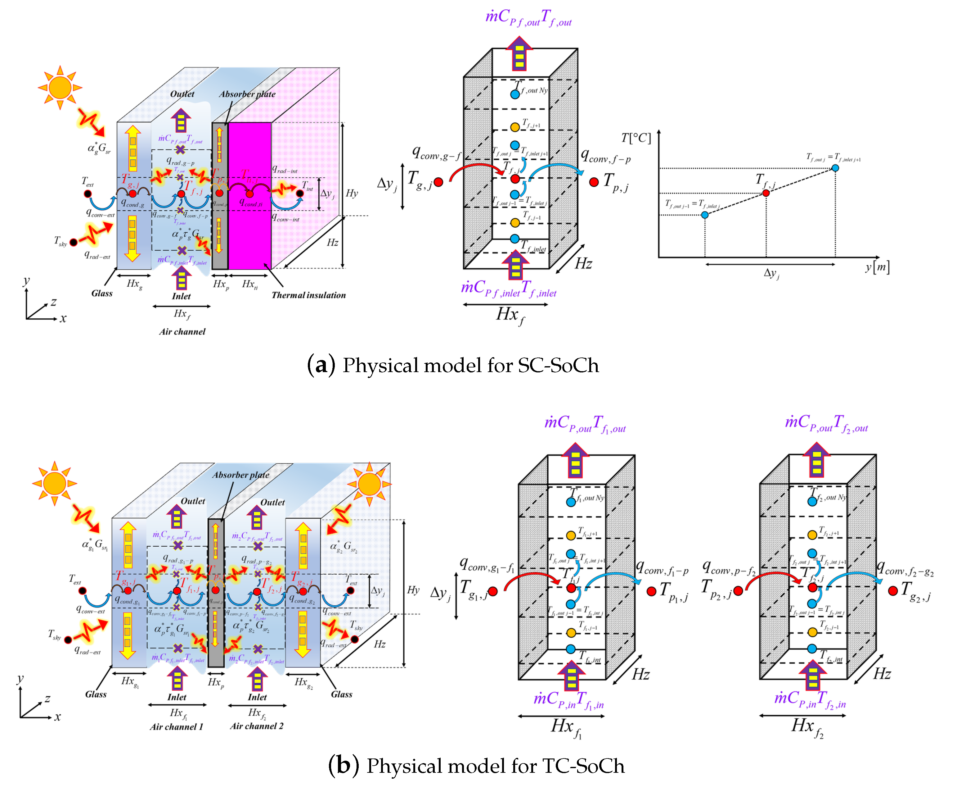
2.1. The Proposed GEB Approach for SC-SoCh and TC-SoCh

The mathematical model reported by Ong [30,32] was used as a reference for developing the solar chimney models. However, the models reported considering the air channel with only one node to state an energy balance. The assumptions considered for SC-SoCh and TC-SoCh models are unsteady-state conditions to evaluate the variations to the climatic conditions and the thermal inertia effect in the induced ventilation; one-dimensional heat transfer is assumed for energy transfer processes through the glass, absorber plate, and thermal insulation, but two-dimensional heat transfer is assumed through the air channel; the temperature of air varies along the height of the channel. Multiple nodes are assumed along the y-direction on solid elements for the air channel; the two-dimensional effect along the height of the channel permits the evaluation of the thermal inertia effect inside the channel, which influences the calculation of the mass flow rate because the empirical correlations depend on the mean temperature of the fluid; in addition, the change in air properties is addressed by considering the temperature change along the height of the channel.

A thermal network analogy is considered to perform the GEB model in each node; the glass cover and absorber plate are parallel; therefore, the section area of the inlet and outlet is the same; temperatures along the width of the channel are equal; airflow in the channel is laminar or turbulent; the air into the channel is non-radiating absorber fluid. Therefore, surface radiative exchange is considered between the parallel plates of the channel; frictional losses were neglected due to the low order of airflow; the glass cover is opaque to infrared radiation; density of air is dependent on temperature, relative humidity, and atmospheric pressure; the sky is considered as a blackbody for long wavelength radiation at the sky temperature; properties of thermal insulation are dependent on temperature; and thermophysical properties are evaluated at an average temperature. Finally, this study evaluates solar chimney models; the room’s or enclosure’s temperature is fixed. Figure 1 shows solar chimney models for SC-SoCh and TC-SoCh. Figure 1a shows the physical models for SC-SoCh, and Figure 1b shows the physical models for TC-SoCh.

2.1.1. GEB Model for SC-SoCh

The SC-SoCh is mainly comprised of a glass cover and absorber plate; both elements create an air channel connected to a room. Therefore, the developed mathematical model of SC-SoCh is suitable for analyzing SC as a façade for any orientation. However, the orientation of SC-SoChs is south for the five cities evaluated. Next, each element of the GEB model, i.e., glass cover, air channel, absorber plate, and thermal insulation, is described.

The glass cover (g) receives and absorbs part of incident solar radiation (${\alpha }_g^{*}{G}_{s}r$); it also absorbs radiation from the absorber plate ($q_{rad,g-p}$) and loses energy by natural convection to air ($q_{conv-ext}$) and radiative transfer to the sky ($q_{rad-ext}$). Heat conduction is considered in the glass cover ($q_{cond,g}$). According to the thermal network analogy, conductive and convective terms are joined, such as thermal resistance. The energy storage term is included to consider the unsteady state in all elements of SC-SoCh. The j subscript is employed to indicate a node in the y-direction because the two-dimensional effect along the height of the channel affects the GEB for the solid elements, which consider the heat transfer in only one direction. Equation (1) describes the energy transfer through the glass cover.   

$$\begin{array}{c}\underset{\mathrm{Convective}-\mathrm{Conductive}\mathrm{thermal}\mathrm{resistance}}{\underbrace{\frac{(T_{ext}-T_{g,j})}{(\frac{1}{h_{conv-ext}}+\frac{H{x}_{g,j}}{2{\lambda }_{g,j}})}}{A}_{g,j}}+\underset{\mathrm{Radiative}\mathrm{thermal}\mathrm{resistance}}{\underbrace{\frac{(T_{sky}-T_{g,j})}{\left(\frac{1}{h_{radg,j-sky}}\right)}}{A}_{g,j}}+\underset{\mathrm{Absorbed}\mathrm{solar}\mathrm{radiation}}{\underbrace{{\alpha }_g^{*}{G}_{sr}{A}_{g,i}}}\hfill \\ -\underset{\mathrm{Convective}-\mathrm{Conductive}\mathrm{thermal}\mathrm{resistance}}{\underbrace{\frac{(T_{g,j}-T_{f,j})}{(\frac{H{x}_{g,j}}{2{\lambda }_{g,j}}+\frac{1}{h_{convg,j-f,j}})}}{A}_{g,j}}+\underset{\mathrm{Radiative}\mathrm{thermal}\mathrm{resistance}}{\underbrace{\frac{(T_{g,j}-T_{p,j})}{\left(\frac{1}{h_{radg,j-p,j}}\right)}}{A}_{g,j}}\hfill \\ =\underset{\mathrm{Energy}\mathrm{storage}}{\underbrace{\left({\rho }_{g,j}{C}_{P,g,j}H{x}_{g,j}{A}_{g,j}\right)\frac{d{T}_{g,j}}{dt}}}\hfill \end{array}$$

(1)

In Equation (1), the term $h_{radg,j-sky}$ is the radiative transfer coefficient between the cover glass and sky; therefore, $h_{radg,j-sky}=\sigma {\epsilon }_g\left(T_{sky}^2+T_{g,j}^2\right)\left(T_{sky}+T_{g,j}\right)$. $h_{radg,j-p,j}$ is the radiative transfer coefficient between the cover glass and the absorber plate, which is obtained through a net radiation transfer model; therefore $h_{radg,j-p,j}=\frac{\sigma \left(T_{g,j}^2+T_{p,j}^2\right)\left(T_{g,j}+T_{p,j}\right)}{\frac{1}{{\epsilon }_g}+\frac{1}{{\epsilon }_p}-1}$. The convective heat transfer coefficients, properties of each element, and overall considerations about numerical modeling are described in Section 2.1.3. In the present study, the energy storage term is substituted by a backward low-order approximation through the finite difference method. Thus, all energy storage terms of this study are expressed as $\frac{dT}{dt}=\frac{\left(T-T^0\right)}{\Delta t}$, where T is the temperature of the current time (t), while $T^0$ is the temperature of the previous time ($t-\Delta t$).

The GEB of the air channel (f) considers the natural convection effect along the height of the channel through the mass flow rate ($\dot{m}{C}_{Pf}{T}_f$) and the convective heat transfer with the glass cover and the absorber plate ($q_{conv,g-f}$ and $q_{conv,f-p}$). Figure 1a shows the reallocation of $T_{f,out}$ and $T_{f,inlet}$ according to j position because the equation is a generic mathematical expression for every node or section inside the air channel. The mass flow rate is the same at the inlet and outlet. A linear relation is performed to relate the air temperatures and the channel height for each j node. Equation (2) describes the GEB of the air channel.

$$\begin{array}{c}\underset{\mathrm{Convective}-\mathrm{Conductive}\mathrm{thermal}\mathrm{resistance}}{\underbrace{\frac{(T_{g,j}-T_{f,j})}{(\frac{H{x}_{g,j}}{2{\lambda }_{g,j}}+\frac{1}{h_{convg,j-f,j}})}}{A}_{g,j}}+\underset{\mathrm{Mass}\mathrm{flow}\mathrm{inlet}}{\underbrace{{\dot{m}}_{inlet}{C}_{Pf,inlet}{T}_{f,inlet}}}-\underset{\mathrm{Convective}-\mathrm{Conductive}\mathrm{thermal}\mathrm{resistance}}{\underbrace{\frac{(T_{f,j}-T_{p,j})}{(\frac{1}{h_{convf,j-p,j}}+\frac{H{x}_{p,j}}{2{\lambda }_{p,j}})}}{A}_{p,j}}\hfill \\ -\underset{\mathrm{Mass}\mathrm{flow}\mathrm{outlet}}{\underbrace{{\dot{m}}_{out}{C}_{Pf,out}{T}_{f,out}}}=\underset{\mathrm{Energy}\mathrm{storage}}{\underbrace{\left({\rho }_{f,j}{C}_{P,f,j}H{x}_{f,j}{A}_{f,j}\right)\frac{d{T}_{f,j}}{dt}}}\hfill \end{array}$$

(2)

Additional considerations are assumed for Equation (2): the mass flow rate and specific heat are constant, along with the height of the control volume ($\Delta y_j$), and the linear relation of $T_{f,j}=\gamma T_{f,out}+\left(1-\gamma \right)T_{f,inlet}$. $\gamma$ is the mean temperature weighting factor of 0.75 for the present study. Therefore, Equation (3) describes the GEB of the air channel under new assumptions.

$$\begin{array}{c}\underset{\mathrm{Convective}-\mathrm{Conductive}\mathrm{thermal}\mathrm{resistance}}{\underbrace{\frac{(T_{g,j}-T_{f,j})}{(\frac{H{x}_{g,j}}{2{\lambda }_{g,j}}+\frac{1}{h_{convg,j-f,j}})}}{A}_{g,j}}+\underset{\mathrm{Mass}\mathrm{flow}}{\underbrace{\dot{m}{C}_{Pf,j}(T_{f,inlet}-T_{f,out})}}-\underset{\mathrm{Convective}-\mathrm{Conductive}\mathrm{thermal}\mathrm{resistance}}{\underbrace{\frac{(T_{f,j}-T_{p,j})}{(\frac{1}{h_{convf,j-p,j}}+\frac{H{x}_{p,j}}{2{\lambda }_{p,j}})}}{A}_{p,j}}\hfill \\ =\underset{\mathrm{Energy}\mathrm{storage}}{\underbrace{\left({\rho }_{f,j}{C}_{P,f,j}H{x}_{f,j}{A}_{f,j}\right)\frac{d{T}_{f,j}}{dt}}}{A}_{g,j}=A_{p,j}=\Delta y_{j}Hz\hfill \end{array}$$

(3)

The absorber plate (p) receives the solar radiation transmitted by the glass cover (${\alpha }_g^{*}{\tau }_g^{*}{G}_{sr}$) and interacts by natural convection to the air ($q_{conv,f-p}$) and by radiative transfer to the glass cover ($q_{rad,g-p}$). Like the glass cover, heat conduction is considered in the absorber plate ($q_{cond,p}$). This element is in contact with thermal insulation to reduce energy losses from the solar chimney. Equation (4) describes the energy transfer through the absorber plates.

$$\begin{array}{c}\underset{\mathrm{Absorbed}\mathrm{solar}\mathrm{radiation}}{\underbrace{{\alpha }_p^{*}{\tau }_g^{*}{G}_{sr}{A}_{p,i}}}+\underset{\mathrm{Convective}-\mathrm{Conductive}\mathrm{thermal}\mathrm{resistance}}{\underbrace{\frac{(T_{f,j}-T_{p,j})}{(\frac{1}{h_{convf,j-p,j}}+\frac{H{x}_{p,j}}{2{\lambda }_{p,j}})}}{A}_{p,j}}+\underset{\mathrm{Radiative}\mathrm{thermal}\mathrm{resistance}}{\underbrace{\frac{(T_{g,j}-T_{p,j})}{\left(\frac{1}{h_{radg,j-p,j}}\right)}}{A}_{p,j}}\hfill \\ -\underset{\mathrm{Convective}-\mathrm{Conductive}\mathrm{thermal}\mathrm{resistance}}{\underbrace{\frac{(T_{p,j}-T_{ti,j})}{(\frac{H{x}_{p,j}}{2{\lambda }_{p,j}}+\frac{H{x}_{ti,j}}{2{\lambda }_{ti,j}})}}{A}_{p,j}}=\underset{\mathrm{Energy}\mathrm{storage}}{\underbrace{\left({\rho }_{p,j}{C}_{P,p,j}H{x}_{p,j}{A}_{p,j}\right)\frac{d{T}_{p,j}}{dt}}}\hfill \end{array}$$

(4)

The GEB of thermal insulation (ti) considers heat conduction ($q_{cond,ti}$), heat convection, and radiation between this element and the internal ambient area or room ($q_{conv,f-p}$ and $q_{rad-int}$) since SC-SoCh can be used as a façade on buildings. Therefore, Equation (5) describes the GEB of thermal insulation.

$$\begin{array}{c}\underset{\mathrm{Conductive}\mathrm{thermal}\mathrm{resistance}}{\underbrace{\frac{(T_{p,j}-T_{ti,j})}{(\frac{H{x}_{p,j}}{2{\lambda }_{p,j}}+\frac{H{x}_{ti,j}}{2{\lambda }_{ti,j}})}}{A}_{ti,j}}-\underset{\mathrm{Convective}-\mathrm{Conductive}\mathrm{thermal}\mathrm{resistance}}{\underbrace{\frac{(T_{ti,j}-T_{int})}{(\frac{H{x}_{ti,j}}{2{\lambda }_{ti,j}}+\frac{1}{h_{conv-int}})}}{A}_{ti,j}}+\underset{\mathrm{Radiative}\mathrm{thermal}\mathrm{resistance}}{\underbrace{\frac{(T_{ti,j}-T_{int})}{\left(\frac{1}{h_{rad-int}}\right)}}{A}_{ti,j}}\hfill \\ =\underset{\mathrm{Energy}\mathrm{storage}}{\underbrace{\left({\rho }_{ti,j}{C}_{P,ti,j}H{x}_{ti,j}{A}_{ti,j}\right)\frac{d{T}_{ti,j}}{dt}}}\hfill \end{array}$$

(5)

In Equation (5), the term $h_{rad-int}$ is the radiative transfer coefficient between the thermal insulation and the internal ambient room area; therefore $h_{rad-int}=\sigma {\epsilon }_{ti}\left(T_{ti,j}^2+T_{int}^2\right)\left(T_{ti,j}+T_{int}\right)$. The convective heat transfer coefficient ($h_{conv-int}$) is described in Section 2.1.3.

2.1.2. GEB Model for TC-SoCh

The TC-SoCh comprises two glass covers and an absorber plate in the middle, which creates two channels; this configuration permits an increase in the heat transfer between the absorber plate and the fluid in the air channels and increases the air volume for natural ventilation. TC-SoCh is suitable for roofs mainly because its configuration permits the exploitation of received energy in both side channels. However, identifying the optimal position of a TC-SoCh on the roof differs from this study’s objective; however, the TC-SoCh is oriented to the north–south for this study. Next, the GEB model is described for each element, i.e., glass covers, air channels, and absorber plate; thermal insulation is not required for this configuration of the solar chimney.

The glass cover 1 ($g_1$) receives and absorbs part of the incident solar radiation (${\alpha }_{g_1}^{*}{G}_{s{r}_1}$); if the glass cover 1 is oriented to the south, then $G_{s{r}_1}$ would be incident solar radiation on that orientation, while $G_{s{r}_2}$ would be incident solar radiation on the north orientation; the model can evaluate the effect of different solar radiation components; however, the method employed to decompose direct and diffuse solar radiation and calculate the incident angle are based on the methodology reported by Duffie and Kalogirou [33,34]. The GEB model of a glass cover considers the energy losses by natural convection to air ($q_{conv-ext}$) and radiative transfer to the sky ($q_{rad-ext}$); also, there is radiative heat transfer between glass cover 1 and the absorber plate ($q_{rad,g_1-p}$). Heat conduction is considered in the glass cover ($q_{cond,g_1}$). According to the thermal network analogy, conductive and convective terms are joined, such as thermal resistance. The energy storage term is included to consider the unsteady state in all elements of SC-SoCh. The j subscript indicates a node in the y-direction, which is the same assumption as for SC-SoCh. Equation (6) describes the energy transfer through glass cover 1 considering the described heat transfer processes.

$$\begin{array}{c}\underset{\mathrm{Convective}-\mathrm{Conductive}\mathrm{thermal}\mathrm{resistance}}{\underbrace{\frac{(T_{ext}-T_{g_1,j})}{(\frac{1}{h_{conv-ext}}+\frac{H{x}_{g_1,j}}{2{\lambda }_{g_1,j}})}}{A}_{g_1,j}}+\underset{\mathrm{Radiative}\mathrm{thermal}\mathrm{resistance}}{\underbrace{\frac{(T_{sky}-T_{g_1,j})}{\left(\frac{1}{h_{rad{g}_1,j-sky}}\right)}}{A}_{g_1,j}}+\underset{\mathrm{Absorbed}\mathrm{solar}\mathrm{radiation}}{\underbrace{{\alpha }_{g_1}^{*}{G}_{s{r}_1}{A}_{g_1,i}}}\hfill \\ -\underset{\mathrm{Convective}-\mathrm{Conductive}\mathrm{thermal}\mathrm{resistance}}{\underbrace{\frac{(T_{g_1,j}-T_{f_1,j})}{(\frac{H{x}_{g_1,j}}{2{\lambda }_{g_1,j}}+\frac{1}{h_{conv{g}_1,j-f_1,j}})}}{A}_{g_1,j}}-\underset{\mathrm{Radiative}\mathrm{thermal}\mathrm{resistance}}{\underbrace{\frac{(T_{g_1,j}-T_{p,j})}{\left(\frac{1}{h_{rad{g}_1,j-p,j}}\right)}}{A}_{g_1,j}}\hfill \\ =\underset{\mathrm{Energy}\mathrm{storage}}{\underbrace{\left({\rho }_{g_1,j}{C}_{P,g_1,j}H{x}_{g_1,j}{A}_{g_1,j}\right)\frac{d{T}_{g_1,j}}{dt}}}\hfill \end{array}$$

(6)

In Equation (6), the term $h_{rad{g}_1,j-sky}$ is the radiative transfer coefficient between glass cover 1 and the sky; therefore $h_{rad{g}_1,j-sky}=\sigma {\epsilon }_{g_1}\left(T_{sky}^2+T_{g_1,j}^2\right)\left(T_{sky}+T_{g_1,j}\right)$. The term $h_{rad{g}_1,j-p,j}$ is a radiative transfer coefficient between glass cover 1 and the absorber plate, which is obtained through a net radiation transfer model; therefore $h_{rad{g}_1,j-p,j}=\frac{\sigma \left(T_{g_1,j}^2+T_{p,j}^2\right)\left(T_{g_1,j}+T_{p,j}\right)}{\frac{1}{{\epsilon }_{g_1}}+\frac{1}{{\epsilon }_p}-1}$. The convective heat transfer coefficients, properties of each element, and overall considerations about numerical modeling are described in Section 2.1.3. Like in the proposed mathematical model of SC-SoCh, the energy storage term is substituted by a backward low-order approximation through the finite difference method.

The GEB of air channel 1 ($f_1$) considers the natural convection effect along the height of the channel through the mass flow rate (${\dot{m}}_1{C}_{P{f}_1}{T}_{f_1}$) and the convective heat transfer with glass cover 1 and the absorber plate ($q_{conv,g_1-f_1}and{q}_{conv,f_1-p}$). Figure 1b shows the reallocation of $T_{f_1,out}$ and $T_{f_1,int}$ according to the j position, which is the same consideration as for the SC-SoCh model. A linear relation is performed to relate the air temperatures and the channel height for each j node. The mass flow rate ${\dot{m}}_1$ corresponds only to the left channel or the channel oriented to the north orientation. Equation (7) describes the GEB of air channel 1.

$$\begin{array}{c}\underset{\mathrm{Convective}-\mathrm{Conductive}\mathrm{thermal}\mathrm{resistance}}{\underbrace{\frac{(T_{g_1,j}-T_{f_1,j})}{(\frac{H{x}_{g_1,j}}{2{\lambda }_{g_1,j}}+\frac{1}{h_{conv{g}_1,j-f_1,j}})}}{A}_{g_1,j}}+\underset{\mathrm{Mass}\mathrm{flow}\mathrm{inlet}}{\underbrace{{\dot{m_1}}_{inlet}{C}_{P{f}_1,inlet}{T}_{f_1,inlet}}}-\underset{\mathrm{Convective}-\mathrm{Conductive}\mathrm{thermal}\mathrm{resistance}}{\underbrace{\frac{(T_{f_1,j}-T_{p,j})}{(\frac{1}{h_{conv{f}_1,j-p,j}}+\frac{H{x}_{p,j}}{2{\lambda }_{p,j}})}}{A}_{p,j}}\hfill \\ -\underset{\mathrm{Mass}\mathrm{flow}\mathrm{outlet}}{\underbrace{{\dot{m_1}}_{out}{C}_{P{f}_1,out}{T}_{f_1,out}}}=\underset{\mathrm{Energy}\mathrm{storage}}{\underbrace{\left({\rho }_{f_1,j}{C}_{P,f_1,j}H{x}_{f_1,j}{A}_{f_1,j}\right)\frac{d{T}_{f_1,j}}{dt}}}{A}_{g_1,j}=A_{p,j}=\Delta y_{j}Hz\hfill \end{array}$$

(7)

As in the GEB model of SC-SoCh, additional considerations are assumed for Equation (7): the mass flow rate and specific heat are constant, along with the height of the control volume ($\Delta y_j$), and there is a linear relation of $T_{f_1,j}=\gamma T_{f_1,out}+\left(1-\gamma \right)T_{f_1,int}$. The value for $\gamma$ is 0.75 for this study, which was obtained during the validation process and coincided with the literature [35]. Therefore, Equation (8) describes the GEB of air channel 1 under new assumptions.   

$$\begin{array}{c}\underset{\mathrm{Convective}-\mathrm{Conductive}\mathrm{thermal}\mathrm{resistance}}{\underbrace{\frac{(T_{g_1,j}-T_{f_1,j})}{(\frac{H{x}_{g_1,j}}{2{\lambda }_{g_1,j}}+\frac{1}{h_{conv{g}_1,j-f_1,j}})}}{A}_{g_1,j}}+\underset{\mathrm{Mass}\mathrm{flow}}{\underbrace{\dot{m_1}{C}_{P{f}_1,j}(T_{f_1,inlet}-T_{f_1,out})}}\hfill \\ -\underset{\mathrm{Convective}-\mathrm{Conductive}\mathrm{thermal}\mathrm{resistance}}{\underbrace{\frac{(T_{f_1,j}-T_{p,j})}{(\frac{1}{h_{conv{f}_1,j-p,j}}+\frac{H{x}_{p,j}}{2{\lambda }_{p,j}})}}{A}_{p,j}}=\underset{\mathrm{Energy}\mathrm{storage}}{\underbrace{\left({\rho }_{f_1,j}{C}_{P,f_1,j}H{x}_{f_1,j}{A}_{f_1,j}\right)\frac{d{T}_{f_1,j}}{dt}}}\hfill \end{array}$$

(8)

Properties of air and the mean temperature weighting factor are described in Section 2.1.3.

For this configuration, the absorber plate (p) is constantly exposed to solar radiation during daylight; this energy is transferred with the fluid of both channels. The absorber plate receives the transmitted solar radiation by glass covers 1 and 2 (${\alpha }_{g_1}^{*}{\tau }_{g_1}^{*}{G}_{s{r}_1}$ and ${\alpha }_{g_2}^{*}{\tau }_{g_2}^{*}{G}_{s{r}_2}$) and transfers energy to the air by natural convection in both channels ($q_{conv,f_1-p}$ and $q_{conv,p-f_2}$) and by radiative transfer to glass covers 1 and 2 ($q_{rad,g_1-p}$ and $q_{rad,p-g_2}$). As in the glass covers, heat conduction is considered in the absorber plate ($q_{cond,p}$). This element is not in contact with thermal insulation like as in SC-SoCh, but TC-SoCh draws on energy losses to increase induced airflow. Equation (9) describes the energy transfer through the absorber plates.

$$\begin{array}{c}\underset{\mathrm{Absorbed}\mathrm{solar}\mathrm{radiation}}{\underbrace{({\alpha }_p^{*}{\tau }_{g_1}^{*}{G}_{s{r}_1}+{\alpha }_p^{*}{\tau }_{g_1}^{*}{G}_{s{r}_2})A_{p,i}}}\hfill \\ +\stackrel{\mathrm{Air}\mathrm{channel}1}{\overbrace{\underset{\mathrm{Convective}-\mathrm{Conductive}\mathrm{thermal}\mathrm{resistance}}{\underbrace{\frac{(T_{f_1,j}-T_{p,j})}{(\frac{1}{h_{conv{f}_1,j-p,j}}+\frac{H{x}_{p,j}}{2{\lambda }_{p,j}})}}{A}_{p,j}}+\underset{\mathrm{Radiative}\mathrm{thermal}\mathrm{resistance}}{\underbrace{\frac{(T_{g_1,j}-T_{p,j})}{\left(\frac{1}{h_{rad{g}_1,j-p,j}}\right)}}{A}_{p,j}}}}\hfill \\ -\stackrel{\mathrm{Air}\mathrm{channel}2}{\overbrace{\underset{\mathrm{Convective}-\mathrm{Conductive}\mathrm{thermal}\mathrm{resistance}}{\underbrace{\frac{(T_{p,j}-T_{f_2,j})}{(\frac{H{x}_{p,j}}{2{\lambda }_{p,j}}+\frac{1}{h_{convp,j-f_2,j}})}}{A}_{p,j}}-\underset{\mathrm{Radiative}\mathrm{thermal}\mathrm{resistance}}{\underbrace{\frac{(T_{p,j}-T_{g_2,j})}{\left(\frac{1}{h_{radp,j-g_2,j}}\right)}}{A}_{p,j}}}}\hfill \\ =\underset{\mathrm{Energy}\mathrm{storage}}{\underbrace{\left({\rho }_{p,j}{C}_{P,p,j}H{x}_{p,j}{A}_{p,j}\right)\frac{d{T}_{p,j}}{dt}}}\hfill \end{array}$$

(9)

If the absorber plate is composed of massive materials like concrete, brick, or a phase-change material, the GEB model would consider multiple nodes or layers to represent thermal storage.

The GEB of air channel 2 ($f_2$) considers the same effects as air channel 1: the natural convection effect along the height of the channel through the mass flow rate (${\dot{m}}_2{C}_{P{f}_2}{T}_{f_2}$) and the convective heat transfer with glass cover 2 and the absorber plate ($q_{conv,f_2-g_2}$ and $q_{conv,p-f_2}$). Figure 1b shows the reallocation of $T_{f_2,out}$ and $T_{f_2,int}$ according to the j position. The mass flow rate ${\dot{m}}_2$ corresponds to the right channel or the channel oriented to the south orientation. A linear relation is performed to relate the air temperatures along the channel height for each j node. Equation (10) describes the GEB of air channel 2.   

$$\begin{array}{c}\underset{\mathrm{Convective}-\mathrm{Conductive}\mathrm{thermal}\mathrm{resistance}}{\underbrace{\frac{(T_{p,j}-T_{f_2,j})}{(\frac{H{x}_{p,j}}{2{\lambda }_{p,j}}+\frac{1}{h_{conv{f}_2,j-p,j}})}}{A}_{p,j}}+\underset{\mathrm{Mass}\mathrm{flow}\mathrm{inlet}}{\underbrace{{\dot{m_2}}_{inlet}{C}_{P{f}_2,inlet}{T}_{f_2,inlet}}}-\underset{\mathrm{Convective}-\mathrm{Conductive}\mathrm{thermal}\mathrm{resistance}}{\underbrace{\frac{(T_{f_2,j}-T_{g_2,j})}{(\frac{1}{h_{conv{f}_2,j-g_2,j}}+\frac{H{x}_{g_2,j}}{2{\lambda }_{g_2,j}})}}{A}_{g_2,j}}\hfill \\ -\underset{\mathrm{Mass}\mathrm{flow}\mathrm{outlet}}{\underbrace{{\dot{m_2}}_{out}{C}_{P{f}_2,out}{T}_{f_2,out}}}=\underset{\mathrm{Energy}\mathrm{storage}}{\underbrace{\left({\rho }_{f_2,j}{C}_{P,f_2,j}H{x}_{f_2,j}{A}_{f_2,j}\right)\frac{d{T}_{f_2,j}}{dt}}}{A}_{g_2,j}=A_{p,j}=\Delta y_{j}Hz\hfill \end{array}$$

(10)

As in the GEB model of SC-SoCh, additional considerations for TC-SoCh are assumed in Equation (10): the mass flow rate and specific heat are constant along with the height of the control volume ($\Delta y_j$), and there is linear relation of $T_{f_2,j}=\gamma T_{f_2,out}+\left(1-\gamma \right)T_{f_2,int}$. Also, the $\gamma$ value is 0.75, as in air channel 1. Therefore, Equation (11) describes the GEB of the air channel under new assumptions.

$$\begin{array}{c}\underset{\mathrm{Convective}-\mathrm{Conductive}\mathrm{thermal}\mathrm{resistance}}{\underbrace{\frac{(T_{p,j}-T_{f_2,j})}{(\frac{H{x}_{p,j}}{2{\lambda }_{p,j}}+\frac{1}{h_{conv{f}_2,j-p,j}})}}{A}_{p,j}}+\underset{\mathrm{Mass}\mathrm{flow}}{\underbrace{\dot{m_2}{C}_{P{f}_2,j}(T_{f_2,inlet}-T_{f_2,out})}}-\underset{\mathrm{Convective}-\mathrm{Conductive}\mathrm{thermal}\mathrm{resistance}}{\underbrace{\frac{(T_{f_2,j}-T_{g_2,j})}{(\frac{1}{h_{conv{f}_2,j-g_2,j}}+\frac{H{x}_{g_2,j}}{2{\lambda }_{g_2,j}})}}{A}_{g_2,j}}\hfill \\ =\underset{\mathrm{Energy}\mathrm{storage}}{\underbrace{\left({\rho }_{f_2,j}{C}_{P,f_2,j}H{x}_{f_2,j}{A}_{f_2,j}\right)\frac{d{T}_{f_2,j}}{dt}}}{A}_{g_2,j}=A_{p,j}=\Delta y_{j}Hz\hfill \end{array}$$

(11)

The GEB for glass cover 2 ($g_2$) considers the same effects as on glass cover 1. The temperatures of the ambient outdoor and the sky used by the GEB model are the same for glass covers 1 and 2. Equation (12) describes the energy transfer through glass cover 1.

$$\begin{array}{c}\underset{\mathrm{Convective}-\mathrm{Conductive}\mathrm{thermal}\mathrm{resistance}}{\underbrace{\frac{(T_{f_2,j}-T_{g_2,j})}{(\frac{1}{h_{conv{f}_2,j-g_2,j}}+\frac{H{x}_{g_2,j}}{2{\lambda }_{g_2,j}})}}{A}_{g_2,j}}+\underset{\mathrm{Radiative}\mathrm{thermal}\mathrm{resistance}}{\underbrace{\frac{T_{p,j}-\left(T_{g_2,j}\right)}{\left(\frac{1}{h_{radp,j-g_2,j}}\right)}}{A}_{g_2,j}}+\underset{\mathrm{Absorbed}\mathrm{solar}\mathrm{radiation}}{\underbrace{{\alpha }_{g_2}^{*}{G}_{s{r}_2}{A}_{g_2,i}}}\hfill \\ -\underset{\mathrm{Convective}-\mathrm{Conductive}\mathrm{thermal}\mathrm{resistance}}{\underbrace{\frac{(T_{g_2,j}-T_{ext})}{(\frac{H{x}_{g_2,j}}{2{\lambda }_{g_2,j}}+\frac{1}{h_{conv-ext}})}}{A}_{g_2,j}}-\underset{\mathrm{Radiative}\mathrm{thermal}\mathrm{resistance}}{\underbrace{\frac{(T_{g_2,j}-T_{sky})}{\left(\frac{1}{h_{rad{g}_2,j-sky}}\right)}}{A}_{g_2,j}}\hfill \\ =\underset{\mathrm{Energy}\mathrm{storage}}{\underbrace{\left({\rho }_{g_2,j}{C}_{P,g_2,j}H{x}_{g_2,j}{A}_{g_2,j}\right)\frac{d{T}_{g_2,j}}{dt}}}\hfill \end{array}$$

(12)

In Equation (12), the term $h_{rad{g}_2,j-sky}$ is the radiative transfer coefficient between glass cover 2 and the sky; therefore $h_{rad{g}_2,j-sky}=\sigma {\epsilon }_{g_2}\left(T_{sky}^2+T_{g_2,j}^2\right)\left(T_{sky}+T_{g_2,j}\right)$. The term $h_{rad{g}_2,j-p,j}$ is the radiative transfer coefficient between glass cover 1 and the absorber plate, which is obtained through a net radiation transfer model; therefore $h_{radp,j-g_2,j}=\frac{\sigma \left(T_{g_2,j}^2+T_{p,j}^2\right)\left(T_{g_2,j}+T_{p,j}\right)}{\frac{1}{{\epsilon }_{g_2}}+\frac{1}{{\epsilon }_p}-1}$. The convective heat transfer coefficients, properties of each element, and overall considerations about numerical modeling are described in Section 2.1.3.

2.1.3. Coefficients for and Properties of Convective Heat Transfer

This section presents the relations to obtain the convective coefficients; thermophysical properties of air in the function of laminar or turbulent flow; the procedure to determine the air density as a function of temperature, relative humidity, and atmospheric pressure; and the correlations to calculate the airflow induced by SC-SoCh and TC-SoCh.

The sky temperature is $T_{sky}=0.00552T_{amb}^{1.5}$; it is given by Swinbank [36].

For this study, convective heat is set to $h_{conv-int}=10 {\mathrm{Wm}}^{-2}{\mathrm{K}}^{-1}$[32]. The term $h_{conv-ext}$ is the average convective heat transfer coefficient between the glass cover and external ambient area, and it is set to $h_{conv-ext}=2.8+3.0V_{wind}$. For this study, the external convective coefficient is a function of the wind velocity ($V_{wind}$ (ms${}^{-1}$)) [37].

The convective heat transfer coefficients between the glass cover and the fluid in the air channel ($h_{convg,j-f,j},h_{conv{g}_1,j-f_1,j}$ and $h_{conv{f}_2,j-g_2,j}$) and between the absorber plate and the fluid of the air channel ($h_{convf,j-p,j},$$h_{conv{f}_1,j-p,j}$ and $h_{convp,j-f_2,j}$) are functions of the convective Nusselt number ($N{u}_{conv}$). Equation (13) describes the convective coefficients for each solar chimney model.

$$\begin{array}{c}\underset{\mathrm{Glass}\mathrm{cover}-\mathrm{Air}}{\underbrace{h_{convg,j-f,j}=\frac{N{u}_{g,j-f,j}{\lambda }_{f,j}}{\Delta y_j}}};\underset{\mathrm{Air}-\mathrm{Absorber}\mathrm{plate}}{\underbrace{h_{convf,j-p,j}=\frac{N{u}_{f,j-p,j}{\lambda }_{f,j}}{\Delta y_j}}};\hfill \\ \underset{\mathrm{Glass}\mathrm{cover}1-\mathrm{Air}:\mathrm{Airchannel}1}{\underbrace{h_{conv{g}_1,j-f_1,j}=\frac{N{u}_{g_1,j-f_1,j}{\lambda }_{f_1,j}}{\Delta y_j}}};\underset{\mathrm{Air}-\mathrm{Absorber}\mathrm{plate}:\mathrm{Airchannel}1}{\underbrace{h_{conv{f}_1,j-p,j}=\frac{N{u}_{f_1,j-p,j}{\lambda }_{f_1,j}}{\Delta y_j}}}\hfill \\ \underset{\mathrm{Absorber}\mathrm{plate}-\mathrm{Air}:\mathrm{Airchannel}2}{\underbrace{h_{convp,j-f_2,j}=\frac{N{u}_{p,j-f_2,j}{\lambda }_{f_2,j}}{\Delta y_j}}};\underset{\mathrm{Air}-\mathrm{Glass}\mathrm{cover}2:\mathrm{Airchannel}2}{\underbrace{h_{conv{f}_2,j-g_2,j}=\frac{N{u}_{f_2,j-g_2,j}{\lambda }_{f_2,j}}{\Delta y_j}}}\hfill \end{array}$$

(13)

In Equation (13), $N{u}_{conv}$ is an experimental correlation reported by Churchill and Chu [38]. This number depends on the Prandtl number ($Pr$) and the Rayleigh number ($Ra$). If $Ra<{10}^9$, the flow is in the laminar regime, and the mathematical expression to compute $N{u}_{conv}$ is set to $N{u}_{conv}=0.68+0.67R{a}^{1/4}/{[1+{(0.492/Pr)}^{9/16}]}^{4/9}$[39]. However, if $Ra>{10}^9$, the flow is in the turbulent regime, and the mathematical expression to compute $N{u}_{conv}$ is set to $N{u}_{conv}={[0.825+0.387R{a}^{1/6}/{[1+{(0.492/Pr)}^{9/16}]}^{8/27}]}^2$. However, the $Ra$ depends on the temperature difference between the glass cover or absorber wall surface and the fluid, which is expressed by the Grashof number ($Gr$) [39]. Equation (14) describes the Grashof number.

$$\begin{array}{c}G{r}_{g,j-f,j}=\frac{g{\beta }_{f,j}\left|T_{g,j}-T_{f,j}\right|\Delta y_j^3}{{\nu }_{f,j}^2};G{r}_{f,j-p,j}=\frac{g{\beta }_{f,j}\left|T_{f,j}-T_{p,j}\right|\Delta y_j^3}{{\nu }_{f,j}^2}\hfill \\ G{r}_{g_1,j-f_1,j}=\frac{g{\beta }_{f_1,j}\left|T_{g_1,j}-T_{f_1,j}\right|\Delta y_j^3}{{\nu }_{f_1,j}^2};G{r}_{f_1,j-p,j}=\frac{g{\beta }_{f_1,j}\left|T_{f_1,j}-T_{p,j}\right|\Delta y_j^3}{{\nu }_{f_1,j}^2}\hfill \\ G{r}_{p,j-f_2,j}=\frac{g{\beta }_{f_2,j}\left|T_{p,j}-T_{f_2,j}\right|\Delta y_j^3}{{\nu }_{f_2,j}^2};G{r}_{f_2,j-g_2,j}=\frac{g{\beta }_{f_2,j}\left|T_{f_2,j}-T_{g_2,j}\right|\Delta y_j^3}{{\nu }_{f_2,j}^2}\hfill \end{array}$$

(14)

In Equation (14), ${\nu }_f$ is the kinematic viscosity of the fluid. It can be expressed as ${\nu }_f=\frac{{\mu }_f}{{\rho }_f}$, ${\beta }_f$ is the thermal expansion coefficient of air, which is expressed as ${\beta }_f=\frac{1}{T_f}$, and g is the gravitational constant [32]. Equations (15) and (16) describe the mathematical expressions of $Pr$ and $Ra$, respectively [40].

$$\begin{array}{c}{Pr}_{f,j}=\frac{C_{Pf,j}{\mu }_{f,j}}{{\lambda }_{f,j}};{Pr}_{f_1,j}=\frac{C_{P{f}_1,j}{\mu }_{f_1,j}}{{\lambda }_{f_1,j}};{Pr}_{f_2,j}=\frac{C_{P{f}_2,j}{\mu }_{f_2,j}}{{\lambda }_{f_2,j}}\hfill \end{array}$$

(15)

$$\begin{array}{c}R{a}_{g,j-f,j}=G{r}_{g,j-f,j}{Pr}_{f,j};R{a}_{f,j-p,j}=G{r}_{f,j-p,j}{Pr}_{f,j}\hfill \\ R{a}_{g_1,j-f_1,j}=G{r}_{g_1,j-f_1,j}{Pr}_{f_1,j};R{a}_{f_1,j-p,j}=G{r}_{f_1,j-p,j}{Pr}_{f_1,j}\hfill \\ R{a}_{p,j-f_2,j}=G{r}_{p,j-f_2,j}{Pr}_{f_2,j};R{a}_{f_2,j-g_2,j}=G{r}_{f_2,j-g_2,j}{Pr}_{f_2,j}\hfill \end{array}$$

(16)

For this study, the physical properties of air, like ${\mu }_f$, ${\lambda }_f$ and $C_{Pf}$, have been assumed to vary linearly with air temperature ($T_f$) [32,41,42]. Equation (17) describes empirical relations validated by Arce et al. [43] over a range from 250 to 400 K.

$$\begin{array}{c}{\mu }_f=\left[2.2078T_f^{0.7756}\right]\times {10}^{-7};\\ {\lambda }_f=\left[0.1723T_f^{0.8812}\right]\times {10}^{-3};\\ C_{P,f}=\left[0.9125T_f^{0.0174}\right]\times {10}^3\end{array}$$

(17)

However, the density of air ${\rho }_f$ does not vary linearly with only air temperature as was the case with the last property. For this study, an empirical relation of ${\rho }_f$ as function of ambient temperature, relative humidity, and atmospheric pressure has been employed to consider the effects of changing air moisture and atmospheric pressure on induced airflow. The procedure to compute the density of air according to Giancomo [44] and Davis [45] is: The first step is to obtain the saturation vapor pressure ($P_{sv}$). Equation (18) expresses mathematically the term, and the enhancement factor f is expressed mathematically in Equation (19).

$$\begin{array}{c}{P}_{sv}=1Pa\times e^{\left(A{T}^2+BT+C+\frac{D}{T}\right)}\hfill \\ A=1.2378847\times {10}^{-5}{ \mathrm{K}}^{-2}\hfill \\ B=-1.9121316\times {10}^{-2}{ \mathrm{K}}^{-1}\hfill \\ C=33.93711047\hfill \\ D=-6.3431645\times {10}^{-3} \mathrm{K}\hfill \end{array}$$

(18)

$$\begin{array}{c}f=\alpha +\beta P+\gamma t^2\hfill \\ \alpha =1.00062\hfill \\ \beta =3.14\times {10}^{-8}{\mathrm{Pa}}^{-1}\hfill \\ \gamma =5.6\times {10}^{-7}{ \mathrm{K}}^{-2}\hfill \end{array}$$

(19)

In Equation (18), T is the air temperature in Kelvin, while t in Equation (19) is the air temperature in Celsius degrees. P is the atmospheric pressure in pascals. Equation (20) computes $P_{sv}$ and f as the mole fraction of water vapor.

$$x_v=RH\times f\times \frac{P_{sv}}{P}$$

(20)

In Equation (20), the term $RH$ is the relative humidity. Finally, Equation (21) describes the compressibility Z.

$$\begin{array}{c}Z=1-\frac{P}{T}\left[\begin{array}{c}{a}_0+a_1\left(T+273.15\right)+a_2{\left(T+273.15\right)}^2\\ +\left(b_0+b_1\left(T+273.15\right)\right)x_v+\left(c_0+c_1\left(T+273.15\right)\right)x_v^2\end{array}\right]+\frac{P^2}{T^2}\left(d+e{x}_v^2\right)\hfill \\ a_0=1.58123\times {10}^{-6}{ \mathrm{KPa}}^{-1}\hfill \\ a_1=-2.9331\times {10}^{-8}{ \mathrm{K}}^{-1}{\mathrm{Pa}}^{-1}\hfill \\ a_2=1.1043\times {10}^{-10}{ \mathrm{K}}^{-1}{ \mathrm{Pa}}^{-1}\hfill \\ b_0=5.707\times {10}^{-6}{ \mathrm{KPa}}^{-1}\hfill \\ b_1=-2.051\times {10}^{-8}{\mathrm{Pa}}^{-1}\hfill \\ c_0=1.9898\times {10}^{-4}{ \mathrm{KPa}}^{-1}\hfill \\ c_1=-2.376\times {10}^{-6}{ \mathrm{Pa}}^{-1}\hfill \\ d=1.83\times {10}^{-11}{ \mathrm{K}}^2{\mathrm{Pa}}^{-2}\hfill \\ e=-0.765\times {10}^{-8}{ \mathrm{K}}^2{\mathrm{Pa}}^{-2}\hfill \end{array}$$

(21)

Equation (22) describes the equation for the density of moist air.

$${\rho }_f=\frac{P{M}_a}{ZRT}\left[1-x_v\left(1-\frac{M_v}{M_a}\right)\right]$$

(22)

In Equation (22), R is the molar gas constant ($8.314510\pm 8.4\times {10}^{-6}\mathrm{J}·{\mathrm{mol}}^{-1}·{\mathrm{K}}^{-1}$), $M_a$ is the molar mass of dry air ($0.028963512440\mathrm{kg}·{\mathrm{mol}}^{-1}$), and $M_v$ is the molar mass of water ($0.018015\mathrm{kg}·{\mathrm{mol}}^{-1}$).

The air mass flow induced by the solar chimney for uniform room air temperature is given by Andersen [46] and Bansal et al. [29]. Equation (23) describes the correlations for airflow.

$$\dot{m}=C_d\frac{{\rho }_{f,out}{A}_{outlet}}{\sqrt{1+\frac{A_{outlet}}{A_{inlet}}}}\sqrt{\frac{2gHy\left(T_{f,mean}-T_{room}\right)}{T_{room}}}$$

(23)

In Equation (23), $A_{outlet}$ and $A_{inlet}$ are the outlet and inlet area, respectively, of the solar chimney openings, $C_d$ is the coefficient of discharge, and $T_{room}$ is the temperature of the room. Equation (24) shows the expressions to compute the volumetric flow rate ($\dot{V}$). Finally, the air changes per hour ($ACH$) is $ACH=\frac{\dot{V}}{Volumeofthebuilding}$.

$$\dot{V}=\frac{\dot{m}}{{\rho }_{f,out}}$$

(24)

Equation (23) permits determining the mass flow rate of SC-SoCh, but for the TC-SoCh, it is necessary to use this correlation for each channel and add both mass flow rates to obtain the total induced ventilation. The same procedure is applied to the volumetric flow rate.

2.1.4. Algorithm of SC-SoCh and TC-SoCh Models

The GEB equations of SC-SoCh and TC-SoCh were solved using a similar algorithm, expressed in Algorithm 1. This algorithm summarizes the main parts of the solution of the algebraic equation system formed by the SC-SoCh and TC-SoCh models.

Algorithm 1 Method for solving SC-SoCh and TC-SoCh

Data:  $Hx$, $Hy$, $Hz$, $\lambda$, $C_P$, $\rho$, ${\alpha }^{*}$, ${\tau }^{*}$, ${\rho }^{*}$, $G_{solar}$, $T_{ext}$, $T_{int}$, $h_{conv}$, $V_{wind}$, $C_d$, $HR$, $P_{atm}$, $ϵ$, $t_{modeling}$, $\Delta t$, $alpha$ 1: Set variables (T), properties, and boundary conditions of system 2: Fill matrix $T=T_{initialcondition}$ 3: Generate mesh along the y-axis $\Delta y=Hy/Ny$ 4: $k=0$ 5: while  $t\le t_{modeling}$  do 6:     Rename matrix $T=T^t$ 7:     $t=k\Delta t$ 8:     while $R_{\varphi }^k\ge ϵ$ do 9:           Rename $T^{*}=T$ 10:         Compute coefficients $a,b,c,...$ 11:         Gauss–Seidel solver T 12:         Relaxation of T 13:         Calculate $\dot{m},\dot{V}$ 14:         Compute error $R_T^k={\sum }_i^N|{\left(a_P{T}_P\right)}^n-{(\sum a_{neighbors}{T}_{neighbors}+b)}^n|$ 15:     end while 16:     $k=k+1$ 17: end while 18: Print temperature matrix (T) and air flow ($\dot{m},\dot{V}$)

The structure of Algorithm 1 permits the solutions for the unsteady state models, which are present for GEB and CFD models. The initial temperature field and the system’s boundary conditions were stated based on climatic conditions; the numerical solution considered three simulation days to achieve the independence of the initial condition because only simulating one day affects the results. The computation of coefficients consists of determining properties and convective and radiative coefficients, which depend on temperature and other climatic conditions. Afterward, the equation systems are ready to be solved using the Gauss–Seidel solver; this iterative solver was selected because both solar chimney models generate non-linear effects, which demand an iterative solution. The relaxation of temperature in the numerical solution was stated to handle any problem in the numerical solution; however, the relaxation coefficient $\alpha$ was 1.0. Therefore, the temperature solution could have been more relaxed because the numerical solutions were obtained without convergence problems.

Furthermore, the relaxation is a necessary step for the study and numerical solution of the heat transfer process in massive materials like phase-change materials. The airflow induced by SC is calculated using temperature information. The residual equation is used for computing the error between iterations. Finally, the temperature and airflow results are printed until the simulation ends.

In numerical studies, the potential sources of error are discretization errors and rounding errors. For this study, the roundoff error was reduced using double precision for all calculations. In contrast, the discretization error was attended to by using a suitable time step obtained by a temporal independence study of the SC-SoCh and TC-SoCh models.

2.2. GEB Model Validation

In this subsection, a summary of the experimental setup, acquisition system, and validation process of the GEB models is described.

The solution methodology and GEB models were validated using experimental data of the SC-SoCh prototype reported in [31]. The SC-SoCh prototype was evaluated under controlled conditions. Figure 2 shows the schematic diagram of the SC-SoCh prototype. The SC-SoCh was installed at the Thermal System Laboratory of Centro Nacional de Investigación y Desarrollo Tecnológico (CENIDET), located in Cuernavaca, Morelos, Mexico ($18°{55}^{\prime }{34.0}^{″}$ N, $99°{13}^{\prime }{50.7}^{″}$ W). The experimental prototype and the acquisition system were installed in a section of restricted access to the laboratory to reduce the disturbances during the study. A triple-layer of thermal insulation (OSB plate–extruded polystyrene–OSB plate) was implemented to reduce heat transfer through the back of the absorber plate and sidewalls; an aluminum sheet reduced radiative exchange between surfaces and sidewalls into the channel. A cover glass of 0.006 m was installed with thermal insulation (extruded polystyrene); the thermal insulation was instrumented to quantify heat flow losses through this envelope. The absorber plate was built to emulate uniform and fixed heat flux conditions over a set area $A_{Plate}$ (1.22 × 0.46 m). The absorber plate was comprised of two galvanized steel pieces containing temperature sensors and wire resistance. The wire resistance was a constantan filament with a resistance of 10.635 $\Omega$ m${}^{-1}$. T-type thermocouples (copper–constantan) with an uncertainty of ±0.5 °C were employed to measure the air temperature, surfaces of thermal insulation, sidewalls, and laboratory. Thermopiles manufactured with T-type thermocouples were installed on the absorber plate and insulation surfaces to measure an average temperature over a specific zone. The thermopiles have an uncertainty of ±0.3 °C. A hot-wire anemometer, model FMA901R-MA OMEGA, was used to measure the airspeed at the inlet of the solar chimney. This sensor has a measurement range of 0.0–2.2 ms${}^{-1}$ with an uncertainty of ±0.0508 ms${}^{-1}$. A BMP180 sensor was used to measure atmospheric pressure. The sensor has an uncertainty of ±0.00035 atm. An analog sensor AMT-1001 was used to monitor relative humidity. This sensor emits an analog signal range of 0.0–3.0 V with an uncertainty of ±5.023 RH%. An AGILENT 34970A digital multimeter with three KEYSIGHT 34901A multiplexer cards was used to collect all variable data for the SC-SOCH. These devices were installed using a shield for sensor connectors to reduce electromagnetic disturbances from electronic and power devices.

The temperatures of the elements, airspeed, relative humidity, and atmospheric pressure data were collected from SC-SoCh and processed to analyze the solar chimney performance; the energy losses through the inlet, outlet, and envelopes; and the airflow induced for different heat fluxes induced in the absorber plate. The details of this collected data, the methodology implemented, and the SC-SoCh prototype performance are described by Torres-Aguilar et al. [31]. The GEB models were validated with the experimental results of SC-SoCh for three different configurations of induced heat flux in the absorber plate of the experimental prototype: 100, 300, and 500 Wm${}^{-2}$. The air channel’s evaluated height and gap were 1.77 and 0.15 m, respectively. The time interval between measurements and for the GEB model was 30 s, while the total evaluation time was 21 h. The root mean square deviation (RMSD) was calculated for the temperature of the absorber plate, the temperature of fluid in the channel, and the volumetric flow rate. Equation (25) describes the RMSD [47].

$$RMSD=\sqrt{\frac{{\sum \left[\left(X_{model}-X_{exp}\right)X_{exp}\right]}^2}{n}}$$

(25)

In Equation (25), $X_{model}$ and $X_{exp}$ are the modeling and experimental results, respectively, and n is the amount of data.

Table 1. RMSD of GEB model.

Parameter	Experimental Evaluation: 100 Wm−2	Experimental Evaluation: 300 Wm−2	Experimental Evaluation: 500 Wm−2
Mass flow rate	11.79%	5.46%	5.04%
Volumetric flow rate	11.25%	6.19%	3.69%
Temperature of fluid	5.11%	8.75%	10.13%
Temperature of absorber plate	3.20%	7.12%	9.67%

shows the RMSD of every parameter compared for each heat flux configuration.

The maximum deviation value of airflow calculations for the present GEB model was 11.79%, and the maximum temperature deviation was 10.13%. Figure 3 compares volumetric flow rate results between experimental and theoretical evaluation for different heat flux configurations.

Figure 3 shows the minimal difference between the induced airflows of the SC-SoCh model and the experimental data in the first hour of the test and simulation. The highest RMSD (11.79%) was obtained for the induced mass flow rate. The maximum RMSD obtained in the present study is lower than the differences reported by Marthur et al. [42] and Duan [48], who reported 23 and 17.4% inaccuracy between their model and experimental data, respectively. Therefore, the accuracy of the present solar chimney models is acceptable and represents an improvement in the proposed models over models reported in the literature.

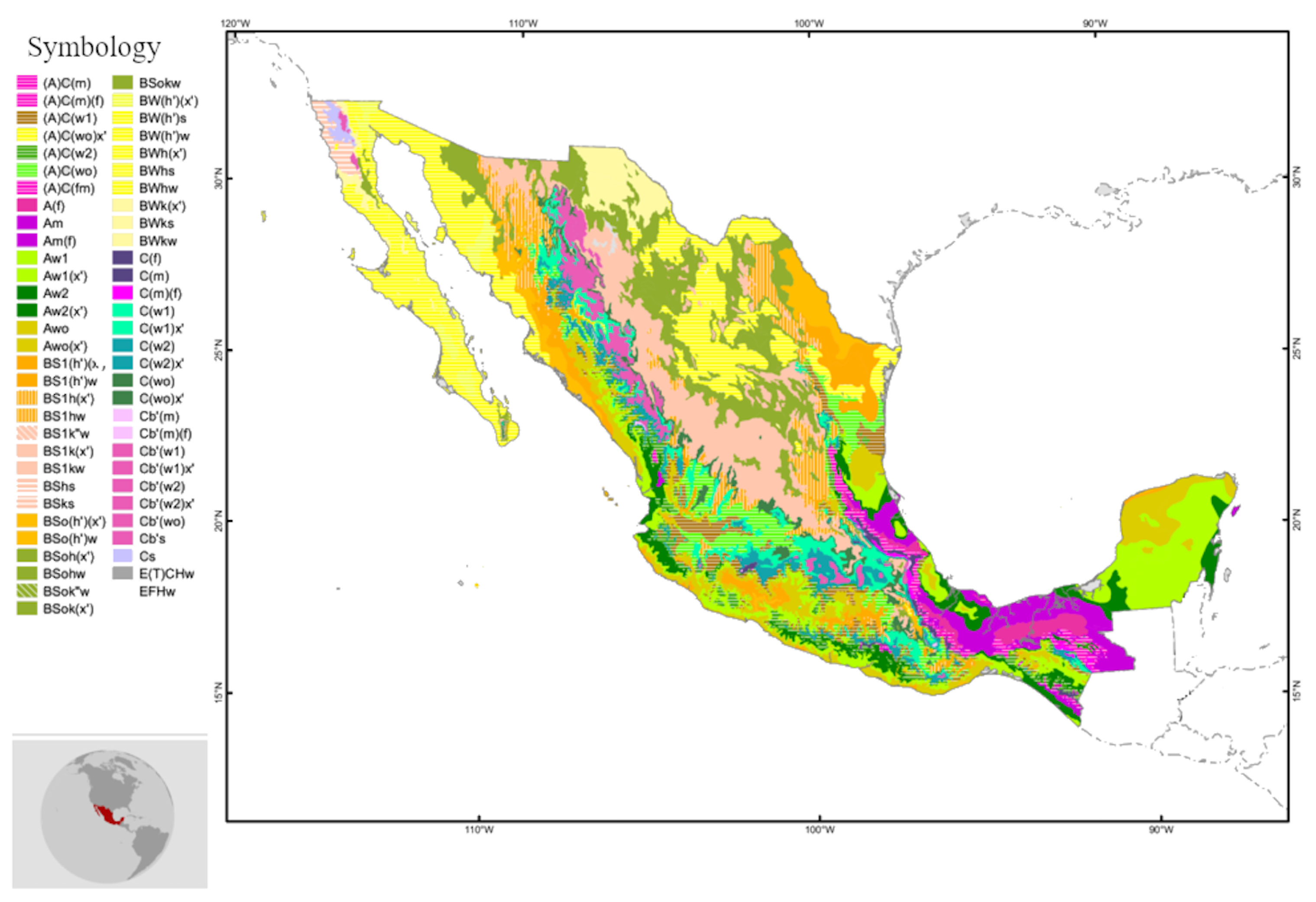
2.3. Parameters of Study: Weather Conditions of Mexico and Considerations for Numerical Modeling

The effect of natural ventilation induced by SC was studied for five weather conditions in Mexico. The selection of the five cities is based on Mexico’s main climatic conditions and their demography, which impact the country’s energy consumption to satisfy ventilation and thermal comfort needs. Mexico is a country with a wide variety of weather. However, according to the INEGI [49], CONABIO [50], and Garcia [51], the A climates (tropical savanna and monsoon), B climates (desert and semi-arid), and C climates (humid subtropical and cool oceanic) are present on 27.7, 49.1, and 23.2% of Mexican territory, respectively. Figure 4 shows the distribution of climates along the Mexican territory. The image was taken from CONABIO and is used only for academic purposes in accordance with the Creative Common license BY-NC 2.5 MX [50].

For this study, five cities of Mexico were selected to evaluate the performance of the SC-SoCh and TC-SoCh for inducing natural ventilation. The selected cities are representative of the main climates of Mexico: Villahermosa (Am) ($17°{59}^{\prime }{12.8}^{″}$ N, $92°55.{817}^{\prime }$ W), Mérida (Aw) ($20°{58}^{\prime }{31.3}^{″}$ N, $89°37.{018}^{\prime }$ W), Hermosillo (BWh) ($29°6^{\prime }{9.4}^{″}$ N, $110°58.{639}^{\prime }$ W), Monterrey (BSh) ($25°{40}^{\prime }{30.3}^{″}$ N, $100°19.{108}^{\prime }$ W), and Mexico City (Cwb) ($19°{25}^{\prime }{42.5}^{″}$ N, $99°7.{66}^{\prime }$ W). The climate data of a typical year were obtained through meteorological stations of Comisión Nacional del Agua (CONAGUA) [52]. Villahermosa and Merida are an exponent of tropical regions; in addition, the populations of these cities is about 683,000 and 995,000 residents, respectively. Hermosillo and Monterrey are dry and semi-arid regions with 936,000 and 1,142,000 residents, respectively. Mexico City and Mexico Valley (metropolitan area) are exponents of humid and sub-humid temperate regions with populations of about 21,800,000 [53]. These cities exposed the need to study the solar chimney performance to contribute to energy saving and help to obtain ventilation for building residents. Two days of every month were selected in all cities to evaluate the warmest and coldest days. The climate data employed were solar radiation, ambient temperature, airspeed, relative humidity, and atmospheric pressure. In addition, the angle of incidence and the components of global solar radiation were obtained using the longitude and latitude of each city and the orientation of SC-SoCh and TC-SoCh considered; Kalogirou [34] and Duffie et al. [33] reported the methodology of this procedure.

The modeling time for every configuration was 72 h of the physical phenomenon; this means that the climate data of a warm or cold day were replicated three times consecutively to obtain independent behavior of the initial condition. The initial temperature of every component of both SCs was established as equal to the ambient temperature. Previous numerical experimentation with both mathematical models revealed that the results of the second day of the numerical modeling were independent of the initial condition; therefore, the results of the first 24 h were discarded, and the analysis was focused on the results of the next 24 h or day. The time interval for the numerical modeling was $\Delta t=5$ s.

The SC-SoCh and TC-SoCh were oriented to the south and north–south in each city. For this study, the values of $C_d$ and $\gamma$ were 0.57 [54] and 0.75 [40], respectively. The mathematical models proposed consider the effect along the y-direction; therefore, the air channel was divided into $Ny$ elements or sections. The air channels for both SCs are $Ny$ = 21. In addition, the dimensions and properties of every element of both SCs are exposed in

Table 2. System parameters for numerical modeling.

	SC-SoCh and TC-SoCh
Height = $Hy$ = 2.0 m Width = $Hz$ = 1.0 m	Air gap = $H{x}_f$ = $H{x}_{f_1}$ = $H{x}_{f_2}$ = 0.15 m	$T_{finlet}=T_{amb}$
Glass cover ${}^1$	Absorber plate (Aluminum with a cover of matte black paint) ${}^2$	Thermal insulation (extruded polystyrene) ${}^3$
$H{x}_g$ = 0.003 m ${\rho }_g$ = 2500 kg m${}^{-3}$ $C_{Pg}$ = 750 J kg${}^{-1}$ K${}^{-1}$ ${\lambda }_g$ = 1.4 W m${}^{-1}$ K${}^{-1}$  ${\alpha }_g^{*}$ = 0.085 ${\tau }_g^{*}$ = 0.838 ${ϵ}_g^{*}$ = 0.840	$H{x}_p$ = 0.0015 m ${\rho }_p$ = 2770 kg m${}^{-3}$  $C_{Pp}$ = 875 J kg${}^{-1}$ K${}^{-1}$  ${\lambda }_p$ = 177 W m${}^{-1}$ K${}^{-1}$  ${\alpha }_p^{*}$ = 0.97 ${ϵ}_p^{*}$ = 0.90	$H{x}_{ti}$ = 0.0508 m ${\rho }_{ti}$ = 21 kg m${}^{-3}$  $C_{Pti}$ = 1210 J kg${}^{-1}$ K${}^{-1}$  ${\lambda }_{ti}$ = 0.0001$T_{ti}$ + 0.0262 W m${}^{-1}$ K${}^{-1}$  ${ϵ}_{ti}^{*}$ = 0.94
	Cases evaluated according to ANSI/ASHRAE 62.2-2019
Configurations	Parameters	Dwelling-unit ventilation
Reference Case	Volume = 27 m${}^3$ Area of floor = 9 m${}^2$ Number of bedrooms = 1	$\dot{V}$ = 30.06 m${}^3$h${}^{-1}$
Case 1	Volume = 54 m${}^3$ Area of floor = 18 m${}^2$ Number of bedrooms = 2	$\dot{V}$ = 47.52 m${}^3$h${}^{-1}$
Case 2	Volume = 108 m${}^3$ Area of floor = 36 m${}^2$ Number of bedrooms = 4	$\dot{V}$ = 82.44 m${}^3$h${}^{-1}$
Case 3	Volume = 162 m${}^3$ Area of floor = 54 m${}^2$ Number of bedrooms = 6	$\dot{V}$ = 117.36 m${}^3$h${}^{-1}$
Case 4	Volume = 216 m${}^3$ Area of floor = 72 m${}^2$ Number of bedrooms = 7	$\dot{V}$ = 152.28 m${}^3$h${}^{-1}$

¹ [39], ² [55], ³ [1].

.

The indicators reported in the ANSI/ASHRAE Standard 62.2-2019 [1] were followed to evaluate the airflow induced by the SC-SoCh and TC-SoCh. Since the standard is focused on residential buildings, the total ventilation rate required for a dwelling unit was obtained for the annual evaluation with both solar chimney models. The ventilation rate reported in the standard corresponds to the capacity of ventilation supplied by mechanical ventilation systems. Therefore, this study aims to analyze the capacity of SCs to induce natural ventilation in residential buildings as a substitute for mechanical systems under Mexican weather conditions.

The ANSI/ASHRAE Standard 62.2-2019 [1] stated that the total ventilation rate is a function of the floor area and the number of bedrooms. Therefore, four cases or configurations were set to analyze the capacity of SC-SoCh and TC-SoCh for providing natural ventilation for residential buildings; the parameters of these cases are stated in Table 2.

The GEB method was described in [25]. The Gauss–Seidel solver was implemented to solve the non-linear equation systems of the SC-SoCh and TC-SoCh models. The convergence criterion employed was 1$\times {10}^{-8}$. The proposed SC-SoCh and TC-SoCh models were developed in ANSI C99 language and compiled with GCC 7.5.0 on GNU/Linux (Ubuntu 18.05, 64 bits). Next, results and discussion are described.

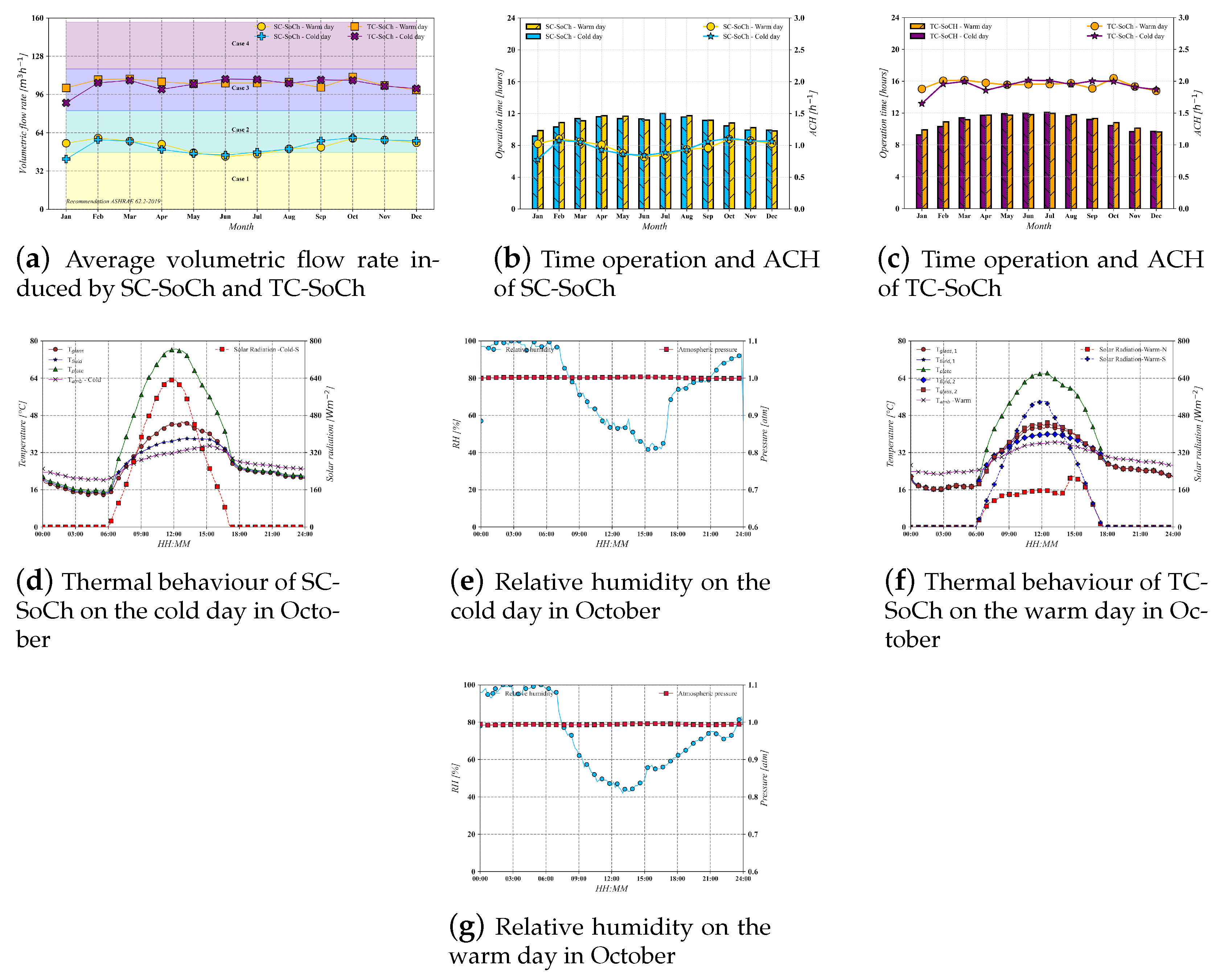
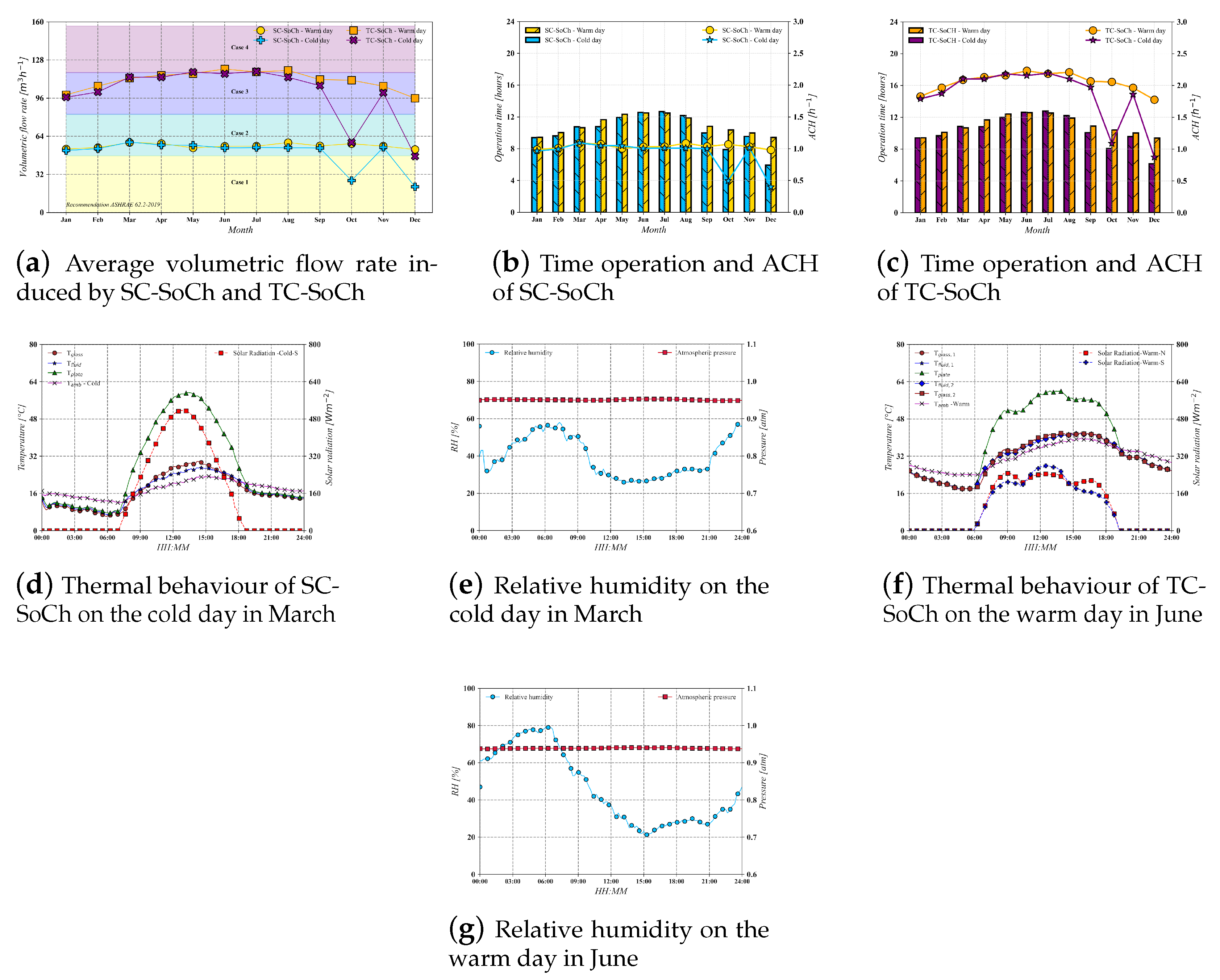
3. Results and Discussion

In this section, the dynamic analysis results are presented for weather conditions in Mexico. The present information corresponds to the annual performance of SC-SoCh and TC-SoCh and their capability for providing natural ventilation according to ASHRAE 62.2-2019 [1]. The annual performance is exposed through the volumetric flow rate, ACH, and operation time of SC-SoCh and TC-SoCh. Comparing both solar chimney configurations permitted the identification of the best solar chimney system for ventilation purposes in every weather condition.

3.1. Am: Villahermosa

A comparison between system performances (SC-SoCh and TC-SoCh) was assessed considering the volumetric flow rate induced by the passive systems. Figure 5a shows the annual performance of solar chimney systems and compares the average volumetric flow rate obtained for warm and cold days. The shaded area indicates the volumetric flow rate required to provide enough ventilation for each case described in Table 2. Results show that the SC-SoCh induces enough natural ventilation for a dwelling unit of two rooms most of the year (Case 1: 47.52 m${}^3$h${}^{-1}$). The performance of SC-SoCh on the cold day in November was the lowest of this evaluation. However, the volumetric flow rate for this day was 33.16 m${}^3$h${}^{-1}$, which is enough to provide enough ventilation for a dwelling unit of 27 m${}^3$ (reference case) according to ASHRAE 62.2-2019.

On the other hand, the highest airflow induced by the SC-SoCh was 56.80 m${}^3$h${}^{-1}$ on the warm day in December. Regarding the performance of the TC-SoCh, Figure 5a shows that the natural ventilation induced by this device almost doubles the airflow achieved by the SC-SoCh. Therefore, the TC-SoCh configuration is ideal to satisfy the ventilation required for a dwelling unit of four rooms most of the year (Case 2: 82.44 m${}^3$h${}^{-1}$) and for a dwelling unit of six rooms (Case 3: 117.36 m${}^3$h${}^{-1}$) from May to July (spring and summer).

Figure 5b,c show the operation time when the solar chimney induces natural ventilation. The maximum operation time registered for the year for SC-SoCh was 12.88 h. In contrast, for the day with the best performance (the warm day in December), the solar chimney worked for 10.09 h. The minimum operation time under this climate was 7.81 h during fall. SC-SoCh was in operation for at least 10 h during the spring and summer seasons (March–August). The operation time of TC-SoCh was like that of SC-SoCh since the maximum operation time was 12.65 h. The TC-SoCh worked more time than the SC-SoCh for most of the year.

The ACH values of Figure 5b,c considered a volume of remotion of 54 m${}^3$ (Case 1). The lowest values of ACH were 0.614 and 1.051 h${}^{-1}$ for SC-SoCh and TC-SoCh, respectively, while the highest values of ACH were 1.051 and 2.206 h${}^{-1}$ for SC-SoCh and TC-SoCh, respectively. The capacity of TC-SoCh to induce natural ventilation and exploit the incident energy was higher than the capacity of SC-SoCh.

Figure 5d,f show the temperature evolution of both SCs, ambient temperature, incident solar radiation on the glass, and relative humidity of the best performance registered: the warm day in December for SC-SoCh and the warm day in May for TC-SoCh. The ambient temperature on both days was similar, in contrast to solar radiation. Incident solar radiation influenced the behavior of the absorber plate temperature more than the ambient temperature. The airflow was also affected by the changes in the relative humidity. Figure 5e shows that the moisture in the air was at its maximum value most of the day; also, Figure 5g shows variations of about 40% for relative humidity. The variation in air moisture directly influences the changes to density and airflow.

The SC-SoCh and TC-SoCh are suitable for inducing natural ventilation in a humid and warm climate. However, the parameters of the SCs in the present study are not optimized, which indicates the capacity to increase the efficiency and benefits obtained through passive systems.

3.2. Aw: Mérida

Figure 6a shows the annual performance of solar chimney devices by comparing the average volumetric flow rates obtained for warm and cold days. SC-SoCh is suitable to induce natural ventilation for a dwelling unit of two rooms most of the year (Case 1: 47.52 m${}^3$h${}^{-1}$). The lowest performance of SC-SoCh was on a cold day in January. The average volumetric flow rate for this day was 41.94 m${}^3$h${}^{-1}$, which was below the necessary rate for Case 1 and is insufficient to provide ventilation for a dwelling unit of 27 m${}^3$ (reference case). The highest average volumetric flow rate induced by SC-SoCh was 59.83 m${}^3$h${}^{-1}$ on the cold day in October.

Figure 6a shows that airflow induced by TC-SoCh was higher than that of SC-SoCh; during some months, the airflow was doubled. Therefore, the TC-SoCh configuration can successfully provide the required ventilation for a dwelling unit of four rooms all year (Case 2: 82.44 m${}^3$h${}^{-1}$), in contrast to the results shown in Section 3.1, but it is not capable of satisfying the required ventilation of Case 3 (117.36 m${}^3$h${}^{-1}$). The highest average volumetric flow rate induced by TC-SoCh was 110.59 m${}^3$h${}^{-1}$ on the warm day in October. However, the parameters of the SC are not optimized for the weather conditions of Merida. Figure 6b,c shows the operation time of both solar chimney systems. The maximum operation time recorded for SC-SoCh was 11.99 h on the cold day in July. The operation time recorded on the cold day in October, the best performance day, was 10.43 h. The minimum operation time was 9.14 h during the winter. The operation time of SC-SoCh during the spring and summer seasons (March–August) was at least 11 h. The operation time tendency of TC-SoCh was like that of SC-SoCh since the maximum operation time was 12.09 h. Although the operation times differed in minutes, TC-SoCh worked more time than SC-SoCh in January–September.

The air volume of Case 1 was considered for computing ACH for the annual evaluation. Figure 6b,c shows variations in the ACH values for SC-SoCh throughout the year compared to those of TC-SoCh. The lowest values of ACH were 0.776 and 1.648 h${}^{-1}$ for SC-SoCh and TC-SoCh, respectively, while the highest values of ACH were 1.108 and 2.048 h${}^{-1}$ for SC-SoCh and TC-SoCh, respectively. The capacity to induce natural ventilation by TC-SoCh is higher than that of SC-SoCh, as in the previous evaluation.

Figure 6d,f show the evolution of both SCs and weather conditions of the best performance registered: the cold day in October for SC-SoCh and the warm day in October for TC-SoCh. Ambient temperature differences were around 2 °C, and relative humidity was similar in both evaluations; therefore, the systems were more sensitive to solar radiation changes. Although the incident solar radiation in the single orientation of SC-SoCh was higher than that of the TC-SoCh configuration, the performance of the latter is better; this behavior highlights the superior efficiency of TC-SoCh over SC-SoCh.

Although the literature and present results suggest that the capability of SC-SoCh to induce natural ventilation under this climate is suitable, an optimal design and implementation of TC-SoCh could be the best option to exploit natural resources and provide more natural ventilation.

3.3. BWh: Hermosillo

The performances of SC-SoCh and TC-SoCh were assessed under dry weather conditions. The thermal comfort of buildings could be affected by the implementation of SCs under these weather conditions; however, preconditioning the air of the inlets, for example, doors and windows, is an alternative to enhance the capacity of SCs to induce natural ventilation.

Figure 7a shows the annual performance of solar chimney systems. The results show that the SC-SoCh induced enough natural ventilation for a dwelling unit of two rooms all year (Case 1: 47.52 m${}^3$h${}^{-1}$); however, its ventilation capacity under the present parameters was not enough to cover the more considerable volume of Case 2. The highest and lowest performances of SC-SoCh were on the warm day in March and the cold day in December, with average volumetric flow rates of 47.78 and 59.14 m${}^3$h${}^{-1}$, respectively.

Figure 7a shows that in May–August, the induced natural ventilation of SC-SoCh was duplicated by TC-SoCh. For the rest of the year, the achieved airflow of TC-SoCh was over 80% higher than that of SC-SoCh. The TC-SoCh capacity covers the minimum requirements of ventilation for a dwelling unit of four rooms all year (Case 2: 82.44 m${}^3$h${}^{-1}$) and a dwelling unit of six rooms (Case 3: 117.36 m${}^3$h${}^{-1}$) from June–August (summer). The highest and lowest performances of TC-SoCh were on the warm day in July and the cold day in December, with average volumetric flow rates of 86.52 and 120.18 m${}^3$h${}^{-1}$, respectively.

Figure 7b,c show SCs’ operation time. The maximum and minimum operation times recorded by the SC-SoCh were 12.38 and 8.56 h, respectively; these behaviors were obtained on the cold day in July and the cold day in December, respectively. The operation time for the day with the highest induced airflow was 10.88 h, which is in the middle of the recorded times. SC-SoCh operated for at least 10 h during the spring and summer (March–September). The tendency of the operation time of TC-SoCh was like that of SC-SoCh; the difference was from 1 to 36 min between both evaluations. During March–August, the operation time of TC-SoCh was higher than the registered time of SC-SoCh. In the cold seasons, the airflow induced by SC-SoCh was superior to that of TC-SoCh.

A volume of 54 m${}^3$ (Case 1) was considered for computing the ACH values: Figure 7b,c. As a result, the lowest values of ACH were 0.884 and 1.602 h${}^{-1}$ for SC-SoCh and TC-SoCh, respectively, while the highest values of ACH were 1.095 and 2.225 h${}^{-1}$, respectively.

Figure 7d,f show the evolution of both SCs for their best registered performances: the warm day in March and the warm day in July for SC-SoCh and TC-SoCh, respectively. Although the temperature of the absorber plate of SC-SoCh was higher than that of TC-SoCh, the induced airflow by TC-SoCh was superior. The induced airflow depends on solar radiation, ambient temperature, and air moisture. However, the temperature of the elements was more sensitive to solar radiation than other parameters. The ambient temperature is a factor for preconditioning the inlet air since it can affect the thermal comfort in a room. On the other hand, the model considered the ambient temperature at the inlet, so the temperature difference between the fluid of the channel and the internal fluid of the room could induce more natural ventilation, which increases the benefits of SCs under dry weather conditions.

3.4. BSh: Monterrey

The Monterrey weather conditions, such as in Hermosillo, are considered dry climates according to García [51].

Figure 8a shows the annual performance of SC-SoCh and TC-SoCh and compares the average volumetric flow rate obtained for warm and cold days. Figure 8a shows that SC-SoCh induces enough natural ventilation for a dwelling unit of two rooms most of the year (Case 1: 47.52 m${}^3$h${}^{-1}$); during the cold days in October and December, the average volumetric flow was insufficient to satisfy the minimum ventilation for a dwelling of 27 m${}^3$ (reference case: 30.06 m${}^3$h${}^{-1}$). The highest and lowest performances of SC-SoCh were obtained for the cold day in March and the cold day in December, respectively; the highest and lowest average volumetric flow rates were 58.98 and 21.53 m${}^3$h${}^{-1}$, respectively.

TC-SoCh induced at least 81% more natural ventilation than that generated by SC-SoCh; the highest difference between both systems was obtained during March–September, when the airflow induced by TC-SoCh was from 92 to 116% higher than that SC-SoCh. The highest and lowest average volumetric flow rates were 120.37 and 58.98 m${}^3$h${}^{-1}$, respectively, and were recorded on the hot day in June and the cold day in December. TC-SoCh provided the required ventilation for a dwelling unit of two rooms most of the year (Case 2: 82.44 m${}^3$h${}^{-1}$) and for a dwelling unit of six rooms (Case 3: 1117.36 m${}^3$h${}^{-1}$) from June to August (summer). However, the capacity to provide natural ventilation dropped abruptly in October and December due to the sensitive systems under the weather conditions. During this drop, TC-SoCh generated sufficient natural ventilation for a dwelling of two rooms (Case 1: 47.52 m${}^3$h${}^{-1}$).

Figure 8b,c show the operation time of both SCs. The maximum and minimum operation times for SC-SoCh were 12.68 and 5.94 h for the cold day in July and the cold day in December, respectively. For the best performance day of SC-SoCh (the cold day in March), the operation time was 10.76 h. The operation time differences between both SCs were below thirteen minutes. Only in January and part of December did the operation time of SC-SoCh exceed that of TC-SoCh. The maximum and minimum operation times for TC-SoCh were 12.78 and 6.14 h for the cold day in July and the cold day in December, respectively. Both systems were affected by October and December weather conditions (fall), specifically during the cold days.

The ACH values in Figure 8b,c considered a volume of remotion of 54 m${}^3$ (Case 1). The lowest values of ACH were 0.398 and 0.873 h${}^{-1}$ for SC-SoCh and TC-SoCh, respectively, while the highest values of ACH were 1.092 and 2.229 h${}^{-1}$ for SC-SoCh and TC-SoCh, respectively. The natural ventilation induced by TC-SoCh was higher than that of SC-SoCh.

Figure 8d,f show the temperature evolution of both SCs, ambient temperature, incident solar radiation on the glass, and relative humidity of the best performance evaluations: the cold day in March for SC-SoCh and the warm day in June for TC-SoCh. Figure 8f shows that the absorber plate of TC-SoCh reached and maintained high temperatures for more time than the absorber plate of SC-SoCh. Although the weather conditions of both evaluations were not the same in March and June, respectively, the temperature evolution showed that the energy received and employed by TC-SoCh was higher than that of SC-SoCh. According to Figure 8, the main differences in relative humidity were before dawn and after sunset. The relative humidity in both cases presented differences of around 5% of relative humidity throughout daylight hours.

3.5. Cwb: Mexico City

Figure 9a shows the annual performance of solar chimney devices by comparing the average volumetric flow rates obtained for warm and cold days. SC-SoCh can induce natural ventilation for a dwelling unit of two rooms most of the year (Case 1: 47.52 m${}^3$h${}^{-1}$). The highest and lowest performances of SC-SoCh were on the cold day in October and the cold day in November, respectively; the average volumetric flow rates obtained on these days were 62.05 and 33.19 m${}^3$h${}^{-1}$, respectively. The lowest induced airflow was enough to provide ventilation for a dwelling unit of 27 m${}^3$ (reference case).

TC-SoCh induced more airflow than SC-SoCh over the year; from May to August, the airflow was doubled. TC-SoCh induced at least 77% more airflow over the year than SC-SoCh. TC-SoCh provided the required ventilation for a dwelling unit of four rooms (Case 2: 88.44 m${}^3$h${}^{-1}$) most of the year except during cold days in November. TC-SoCh provided ventilation for a dwelling of six rooms (Case 3: 11.36 m${}^3$h${}^{-1}$) during the warm days in February and September and the cold days in July. The highest average volumetric flow rate induced by TC-SoCh was 118.99 m${}^3$h${}^{-1}$ on the warm day in September, while the lowest airflow induced was 72.06 m${}^3$h${}^{-1}$ on the cold day in November.

Figure 9b,c show the operation times of both solar chimney systems. The maximum and minimum operation times recorded for SC-SoCh were 12.46 and 9.19 h on the warm day in June and the cold day in November, respectively. The operation time recorded on the cold day in October, the best performance day, was 10.77 h. The operation time of SC-SoCh during the spring and summer seasons (March–August) was at least 11 h. Similar behavior of operation times of TC-SoCh were registered; the maximum operation time difference of all year between both solar chimney models was 11.5 min. From March to September, the operation time of TC-SoCh was higher than that of SC-SoCh. Only in October and December was the operation of SC-SoCh superior. The maximum operation time of TC-SoCh was 12.51 h on a cold day in June.

The air volume of Case 1 was considered for computing ACH for the annual evaluation. Figure 9b,c show the variations in the ACH values in SC-SoCh in contrast to those of TC-SoCh throughout the year. The highest and lowest values of ACH for SC-SoCh were 0.614 and 1.149 h${}^{-1}$, respectively, while for TC-SoCh, they were 1.334 and 2.203 h${}^{-1}$, respectively. As in the previous evaluation, the capacity to induce natural ventilation by TC-SoCh is higher than that of SC-SoCh under these weather conditions.

Figure 9d,f show the evolution of both SCs and weather conditions of the best performance evaluated: the cold day in October for SC-SoCh and the warm day in September for TC-SoCh. The SCs were more sensitive to solar radiation since the temperature evolution of the absorber plate had the same tendency as the solar radiation. In addition, the temperature difference between inlet air and the external ambient air increased the induced airflow.

An optimal design and implementation of SC-SoCh and TC-SoCh could improve both systems’ capacities to induce natural ventilation under these weather conditions, which would be a feasible alternative.

3.6. Discussion

The annual evaluation of SC-SoCh and TC-SoCh under climate conditions of Mexico revealed that this passive ventilation system induces enough natural ventilation to satisfy the primary conditions of a dwelling unit. Although the design parameters of both SCs are not optimized, the performance over the year shows the potential benefits as a substitute for mechanical systems.

The performances of SC-SoCh and TC-SoCh were enough to satisfy the dwelling-unit ventilation required by the reference case (27 m${}^3$) for the five cities evaluated. However, the differences between both configuration’s performances are remarkable. The performance of TC-SoCh was higher than SC-SoCh in all configurations. TC-SoCh induced from 75% to 80% more airflow than SC-SoCh for Merida, Villahermosa, and Hermosillo weather conditions; for the rest, the increment of induced airflow was above 70% at a minimum. The performance variations between SC-SoCh and TC-SoCh were consequences of climatic condition variations, but the most evident difference was the increment of the energy capture area, which increases the sensible heat and the heat transfer rate inside the air channel; the weather data used in the models involved diffuse and direct solar radiation, which favored the TC-SoCh configuration because during the daylight, one channel received diffuse and direct solar radiation like the air channel of SC-SoCh, but the other air channel of TC-SoCh received diffuse solar energy, increasing energy capture to induce airflow. However, the performance difference obtained showed a nonlinear thermal effect in the airflow induced by the solar chimneys due to air channel arrangement and material properties, an effect reported for SC-SoCh and TC-SoCh in steady-state models [23]. The features of SC-SoCh make it a preferred choice to be implemented in buildings because SC-SoCh uses a façade which requires less modification to the building construction; in contrast, the TC-SoCh configuration is required to be installed on the roof, which supposes more modifications and difficulties to customers for installation. This way, more parametric studies about SC-SoCh are required to optimize the parameters, which increases the thermal performance for inducing more airflow. The thermal behavior of both SCs depends on climate conditions directly. However, it is necessary to couple the SC to a room and to consider other parameters like infiltration, thermal sources, and human activities in the building to evaluate the interactions between these features with the SC-SoCh and TC-SoCh.

Regarding the weather effect on SCs, the evaluation of five climatic conditions showed that the solar radiation and relative humidity are remarkable. Villahermosa and Merida have high relative humidity and solar radiation (Am and Aw). However, the maximum mean airflows induced by SC-SoCh and TC-SoCh were lower than those for the evaluation under Monterrey and Hermosillo climates (BSh and BWh). SCs were affected by the air’s moisture because the specific air volume of humid air is lower than that of the air of dry regions. Therefore, the thermosyphon effect was reduced in humid regions, reducing airflows. Moreover, the mean airflows induced by SC-SoCh and TC-Soch were satisfactory for the reference case building. An extensive parametric study of SC-SoCh and TC-SoCh is needed to obtain the maximum capabilities of these passive ventilation systems. In addition, the present study only focused on ventilation purposes, and a thermal comfort evaluation requires an evaluation considering the room model coupled to the solar chimney to consider the exact effects of the temperature and relative humidity.

On the other hand, although the TC-SoCh is more efficient in receiving and exploiting solar radiation than the SC-SoCh, the operation time of the TC-SoCh was not always superior to the operation time of the SC-SoCh. This behavior is because the low thermal mass of the absorber plate induced a minimal thermal storage effect. Therefore, the evolution of absorber plate temperature was mainly influenced by solar radiation. The operation time registered for SC-SoCh and TC-SoCh is enough for workspaces such as offices, schools, and shopping centers, which demand high ventilation during daylight; these results were anticipated because the absorber plate is a thin metal sheet. However, the delay effect in both SC models was insignificant compared to the effect for massive absorber plates as reported by Li et al. [56] and Ke et al. [15]. This effect is desirable in warm and humid climates where natural ventilation is required after sunset. Therefore, studying mass thermal effects of SCs under weather conditions in Mexico can help to increase the natural ventilation induced by these passive systems.

The volumetric flow rates calculated over the year in Monterrey and Hermosillo were the highest of the present study (up to 120 m${}^3$h${}^{-1}$). However, the evaluation of SC-SoCh and TC-SoCh in these locations shows the importance of air preconditioning before its entrance into the room since the ambient temperature of these locations is higher than in other cities with temperate climates. Therefore, it is necessary to study the implementation of a water sprayer to reduce the negative impact of ambient temperature on thermal comfort.

As discussed, the weather conditions over the year affected the performance of the SC-SoCh and TC-SoCh; during the autumn (October and November), the highest drops in induced airflow were registered in the annual evaluation of Villahermosa, Monterrey, and Mexico City. These behaviors exposed the necessity to evaluate SCs annually and understand their limitations in order to optimize current designs.

4. Conclusions

This article presented a case study of natural ventilation induced by the SC-SoCh and TC-SoCh under tropical, dry, and temperate climates of Mexico in the context of energy efficiency analysis. The proposed mathematical models are based on the GEB method for analyzing the ventilation capacity of two solar chimney configurations in an unsteady state. Both models considered solar radiation, ambient temperature, wind speed, relative humidity, and atmospheric pressure to improve result accuracy.

The studied systems considered climatic data from five cities (Villahermosa, Mérida, Hermosillo, Monterrey, and Mexico City) of Mexico provided by the Comisiń Nacional de Agua. The experimental evaluation was performed by considering the warmest and coldest days of every month of the year. Both solar chimney configurations considered using only metal absorber plates with exact dimensions of airgaps and height. The proposed mathematical model and methodology were compared through experimental results obtained by the solar chimney prototype reported in [31]. Experimental validation showed an improvement, with RMSD values of mass flow rate and volumetric flow rate from 3.69 to 11.79%; we included the effect of the moisture in the air and the change in atmospheric pressure in contrast with other reported mathematical models. The proposed models considered only the effect of surface radiative exchange in the air channel and with the sky.

The main results indicate that the tested TC-SoCh configurations induced at least 70% more airflow than SC-SoCh. The SC-SoCh and TC-SoCh airflows were higher than the dwelling-unit ventilation for a space of 54 m${}^3$ reported by international standards. The highest volumetric flows were up to 120 m${}^3$h${}^{-1}$ for the cities of Hermosillo and Monterrey due to the solar radiation and the low moisture content in the air. The air moisture affects the performance of SC-SoCh and TC-SoCh in tropical weather. The studied configuration provided natural ventilation in buildings as a renewable alternative to reduce energy consumption, reducing CO${}_2$ emitted into the environment by not using active systems or electrical devices to provide ventilation.

It is essential to recognize that implementing any passive system technology in the real world is a challenge due to the paradigm in building design and the practicality of active systems to satisfy ventilation needs and thermal comfort. This study exposed the capabilities of SC-SoCh and TC-SoCh to provide natural ventilation in buildings under different climatic conditions as a substitute for mechanical fans and other electrical devices. The construction cost and maintenance depend on the region and country. However, these passive ventilation systems are an alternative to reduce energy consumption and electrical bills. Also, their zero emission of pollutants is a valuable feature.

The main lines for future work are oriented towards performing a parametric study to determine the ventilation capacity of SC-SoCh and TC-SoCh by varying materials for the absorber plate, such as masonry and phase-change materials; increasing the height and air gap of the channel; and measuring the performance of solar chimneys coupled to a building to evaluate the induced ventilation and strategies oriented to improve thermal comfort. Also, the proposed methodology could extend to a performance study using phase-change materials to increase the operation time of SCs and natural ventilation. Likewise, study of energy consumption costs and pollution emission impacts is relevant.

References

1. ANSI/ASHRAE 62.2-2019. Ventilation for Acceptable Indoor Air Quality in Residential Buildings. 2019. Available online: https://www.ashrae.org/about/news/2019/ashrae-releases-updated-versions-of-standard-62-1-and-62-2 (accessed on 15 November 2023).
2. Roh, T.; Moreno-Rangel, A.; Baek, J.; Obeng, A.; Hasan, N.T.; Carrillo, G. Indoor Air Quality and Health Outcomes in Employees Working from Home during the COVID-19 Pandemic: A Pilot Study. Atmosphere 2021, 12, 1665. [Google Scholar] [CrossRef]
3. Kumar, A.; Moreno-Rangel, A.; Khan, M.A.I.; Piasecki, M. Ventilation and Indoor Air Quality. Atmosphere 2022, 13, 1730. [Google Scholar] [CrossRef]
4. Mata, T.M.; Martins, A.A.; Calheiros, C.S.C.; Villanueva, F.; Alonso-Cuevilla, N.P.; Gabriel, M.F.; Silva, G.V. Indoor Air Quality: A Review of Cleaning Technologies. Environments 2022, 9, 118. [Google Scholar] [CrossRef]
5. Lavtižar, K.; Fikfak, A.; Fink, R. Overlooked Impacts of Urban Environments on the Air Quality in Naturally Ventilated Schools Amid the COVID-19 Pandemic. Sustainability 2023, 15, 2796. [Google Scholar] [CrossRef]
6. Awbi, H. Ventilation of Buildings. 2003. Available online: https://www.taylorfrancis.com/books/mono/10.4324/9780203634479/ventilation-buildings-awbi (accessed on 15 November 2023).
7. Wang, Z.; Wang, Y.; Zeng, R.; Srinivasan, R.S.; Ahrentzen, S. Random Forest based hourly building energy prediction. Energy Build. 2018, 171, 11–25. [Google Scholar] [CrossRef]
8. International Energy Agency. Key World Energy Statistics; International Energy Agency: Paris, France, 2019. [Google Scholar]
9. International Energy Agency. Energy Efficiency; International Energy Agency: Paris, France, 2020. [Google Scholar]
10. International Energy Agency. Energy Efficiency; International Energy Agency: Paris, France, 2021. [Google Scholar]
11. Secretaría de Energía. Programa para el Desarrollo del Sistema Eléctrico Nacional 2022–2036; Secretaría de Energía: Mexico City, Mexico, 2022. [Google Scholar]
12. Instituto Nacional de Estadística y Geografía. Primera Encuesta Nacional Sobre Consumo de Energéticos en Viviendas Particulares (ENCEVI); Instituto Nacional de Estadística y Geografía: Mexico City, Mexico, 2018. [Google Scholar]
13. Abdeen, A.; Serageldin, A.A.; Ibrahim, M.G.; El-Zafarany, A.; Ookawara, S.; Murata, R. Solar chimney optimization for enhancing thermal comfort in Egypt: An experimental and numerical study. Sol. Energy 2019, 180, 524–536. [Google Scholar] [CrossRef]
14. Li, Y.; Long, T.; Bai, X.; Wang, L.; Li, W.; Liu, S.; Lu, J.; Cheng, Y.; Ye, K.; Huang, S. An experimental investigation on the passive ventilation and cooling performance of an integrated solar chimney and earth–air heat exchanger. Renew. Energy 2021, 175, 486–500. [Google Scholar] [CrossRef]
15. Ke, W.; Ji, J.; Xu, L.; Yu, B.; Tian, X.; Wang, J. Numerical study and experimental validation of a multi-functional dual-air-channel solar wall system with PCM. Energy 2021, 227, 120434. [Google Scholar] [CrossRef]
16. Correia-da Silva, J.; Silva, A.; De Oliveira Fernandes, E. Passive Cooling in Livestock Buildings. In Proceedings of the Seventh International IBPSA Conference, IBPSA, Rio de Janeiro, Brazil, 13–15 August 2001; pp. 215–218. [Google Scholar]
17. Raman, P.; Mande, S.; Kishore, V. A passive solar system for thermal comfort conditioning of buildings in composite climates. Sol. Energy 2001, 70, 319–329. [Google Scholar] [CrossRef]
18. Chungloo, S.; Limmeechokchai, B. A field study of free convection in an inclined-roof solar chimney. ScienceAsia 2009, 35, 189–195. [Google Scholar] [CrossRef]
19. Salata, F.; Alippi, C.; Tarsitano, A.; Golasi, I.; Coppi, M. A First Approach to Natural Thermoventilation of Residential Buildings through Ventilation Chimneys Supplied by Solar Ponds. Sustainability 2015, 7, 9649–9663. [Google Scholar] [CrossRef]
20. Yuan, P.; Fang, Z.; Wang, W.; Chen, Y.; Li, K. Numerical Simulation Analysis and Full-Scale Experimental Validation of a Lower Wall-Mounted Solar Chimney with Different Radiation Models. Sustainability 2023, 15, 11974. [Google Scholar] [CrossRef]
21. Arce, J.; Xamán, J.; Alvarez, G.; Jiménez, M.; Guzmán, J.; Heras, M. Theoretical study on a diurnal solar chimney with double air flow. In Proceedings of the 1st International Conference on Solar Heating, Cooling and Buildings (EUROSUN). Sociedade Portuguesa de Energia Solar (SPES), Lisbon, Portugal, 7–10 October 2008; pp. 1–8. [Google Scholar]
22. Tlatelpa-Becerra, A. Estudio de la Transferencia de Calor en una Chimenea Solar para Uso Diurno con Doble Canal de Aire. Master’s Thesis, Cenidet, Cuernavaca, Mexico, 2011. [Google Scholar]
23. Zavala-Guillén, I.; Xamán, J.; Hernández-Pérez, I.; Hernández-Lopéz, I.; Gijón-Rivera, M.; Chávez, Y. Numerical study of the optimum width of 2a diurnal double air-channel solar chimney. Energy 2018, 147, 403–417. [Google Scholar] [CrossRef]
24. Jiménez-Xamán, C.; Xamán, J.; Gijón-Rivera, M.; Zavala-Guillén, I.; Noh-Pat, F.; Simá, E. Assessing the thermal performance of a rooftop solar chimney attached to a single room. J. Build. Eng. 2020, 31, 101380. [Google Scholar] [CrossRef]
25. Torres-Aguilar, C.; Moreno-Bernal, P.; Xamán, J.; Nesmachnow, S.; Cisneros-Villalobos, L. Global energy balances for energy analysis in buildings. In Proceedings of the V Ibero-American Congress of Smart Cities, Cuenca, Ecuador, 28–30 November 2022; pp. 306–320. [Google Scholar]
26. Tariq, R.; Torres-Aguilar, C.; Sheikh, N.A.; Ahmad, T.; Xamán, J.; Bassam, A. Data engineering for digital twining and optimization of naturally ventilated solar façade with phase changing material under global projection scenarios. Renew. Energy 2022, 187, 1184–1203. [Google Scholar] [CrossRef]
27. Cardenas, M.; Tlatelpa-Becerro, A.; Rico-Martínez, R.; Urquiza, G.; Alarcón Hernández, F.; Fuentes-Albarran, M. Prediction of the dynamic behavior of a solar chimney by means of artificial neural networks. Rev. Mex. Ing. Quim. 2022, 21, 1–16. [Google Scholar]
28. Awbi, H.; Gan, G. Simulation of solar-induced ventilation. Dep. Constr. Manag. Eng. 1992, 1, 2016–2030. [Google Scholar]
29. Bansal, N.; Mathur, R.; Bhandari, M. Solar Chimney for Enhanced Stack Ventilation. Build. Environ. 1993, 28, 373–377. [Google Scholar] [CrossRef]
30. Ong, K. Thermal performance of solar air heaters: Mathematical model and solution procedure. Sol. Energy 1995, 55, 93–109. [Google Scholar] [CrossRef]
31. Torres-Aguilar, C.E.; Arce, J.; Xamán, J.; Macias-Melo, E. Experimental study and numerical analysis of radiative losses of single-channel solar chimney. J. Build. Phys. 2022, 46, 340–371. [Google Scholar] [CrossRef]
32. Ong, K. A mathematical model of a solar chimney. Energy 2003, 28, 1047–1060. [Google Scholar] [CrossRef]
33. Duffie, J.; Beckman, W. Solar Engineering of Thermal Processes, 4th ed.; Wiley: Hoboken, NJ, USA, 2013. [Google Scholar]
34. Kalogirou, S. Solar Energy Engineering: Processes and Systems, 4th ed.; Academic Press: Cambridge, MA, USA, 2009. [Google Scholar]
35. Chantawong, P.; Hirunlabh, J.; Zeghmati, B.; Khedari, J.; Teekasap, S.; Win, M.M. Investigation on thermal performance of glazed solar chimney walls. Sol. Energy 2006, 80, 288–297. [Google Scholar] [CrossRef]
36. Swinbank, W. Long-wave radiation from clear skies. Q. J. R. Meteorol. Soc. 1963, 89, 339–348. [Google Scholar] [CrossRef]
37. McAdams, W. Heat Transmission, 1st ed.; McGraw-Hill: New York, NY, USA, 1954. [Google Scholar]
38. Churchill, S.W.; Chu, H. Correlating equations for laminar and turbulent free convection from a horizontal cylinder. Int. J. Heat Mass Transf. 1975, 18, 1049–1053. [Google Scholar] [CrossRef]
39. Bergman, T.L.; Lavine, A.S.; Incropera, F.P.; DeWitt, D.P. Fundamentals of Heat and Mass Transfer, 8th ed.; Wiley: Hoboken, NJ, USA, 2018. [Google Scholar]
40. Martí, J.; Heras-Celemin. Dynamic physical model for a solar chimney. Sol. Energy 2007, 81, 614–622. [Google Scholar] [CrossRef]
41. Bansal, N.; Mathur, J.; Mathur, S.; Jain, M. Modeling of window-sized solar chimneys for ventilation. Build. Environ. 2005, 40, 1302–1308. [Google Scholar] [CrossRef]
42. Mathur, J.; Bansal, N.; Jain, M. Experimental investigations on solar chimney for room ventilation. Sol. Energy 2006, 80, 927–935. [Google Scholar] [CrossRef]
43. Arce, J.; Xamán, J.; Alvarez, G.; Jiménez, M.; Enríquez, R.; Heras, M. A Simulation of the Thermal Performance of a Small Solar Chimney Already Installed in a Building. J. Sol. Energy Eng. 2013, 135, 011005-1–011005–10. [Google Scholar] [CrossRef]
44. Giacomo, P. Equation for the determination of the density of moist air. Metrologia 1982, 18, 33–40. [Google Scholar] [CrossRef]
45. Davis, R. Equation for the determination of the density of moist air. Metrologia 1992, 29, 67–70. [Google Scholar] [CrossRef]
46. Andersen, K. Theoretical considerations on natural ventilation by thermal buoyancy. Ashrae 1995, 101, 1103–1117. [Google Scholar]
47. Ke, W.; Ji, J.; Wang, C.; Zhang, C.; Xie, H.; Tang, Y.; Lin, Y. Comparative analysis on the electrical and thermal performance of two CdTe multi-layer ventilated windows with and without a middle PCM layer: A preliminary numerical study. Renew. Energy 2022, 189, 1306–1323. [Google Scholar] [CrossRef]
48. Duan, S. A predictive model for airflow in a typical solar chimney based on solar radiation. J. Build. Eng. 2019, 26, 100916. [Google Scholar] [CrossRef]
49. INEGI. Guía para la Interpretación de Cartografía Climatológica; Instituto Nacional de Estadistica, Geografia e Informatica: Mexico City, Mexico, 2005. [Google Scholar]
50. CONABIO. Sistema Nacional de Información sobre Biodiversidad (SNIB); Comision Nacional para el Conocimiento y Uso de la Biodiversidad: Mexico City, Mexico, 2023. [Google Scholar]
51. García, E. Modificaciones al Sistema de Clasificación Climática de Köppen, 1st ed.; Universidad Nacional Autónoma de México: Mexico City, Mexico, 2004. [Google Scholar]
52. CONAGUA. Estaciones Meteorológicas Automáticas (EMAS); Comision Nacional del Agua: Mexico City, Mexico, 2023. [Google Scholar]
53. INEGI. Censo de Población y Vivienda 2020; Instituto Nacional de Estadistica, Geografia e Informatica: Aguascalientes, Mexico, 2020. [Google Scholar]
54. Jianliu, X.; Weihua, L. Study on solar chimney used for room natural ventilation in Nanjing. Energy Build. 2013, 66, 467–469. [Google Scholar] [CrossRef]
55. ASTM C578-01; Standard Specification for Rigid, Cellular Polystyrene Thermal Insulation. ASTM International: West Conshohocken, PA, USA, 2002.
56. Li, Y.; Liu, S.; Lu, J. Effects of various parameters of a PCM on thermal performance of a solar chimney. Appl. Therm. Eng. 2017, 127, 1119–1131. [Google Scholar] [CrossRef]
Figure 1. SC-SoCh and TC-SoCh physical models.
Sustainability 15 16399 g001
Figure 2. SC-SoCh schematic diagram.
Sustainability 15 16399 g002
Figure 3. Comparison between experimental and theoretical volumetric flow rates.
Sustainability 15 16399 g003
Figure 4. Mexico map of Köppen climate classifications.
Sustainability 15 16399 g004
Figure 5. Annual performance in tropical climate (Am, Villahermosa).
Sustainability 15 16399 g005
Figure 6. Annual performance in tropical climate (Aw, Mérida).
Sustainability 15 16399 g006
Figure 7. Annual performance in dry climate (BWh, Hermosillo).
Sustainability 15 16399 g007
Figure 8. Annual performance in dry climate (BSh, Monterrey).
Sustainability 15 16399 g008
Figure 9. Annual performance in temperate climate (Cwb, Mexico City).
Sustainability 15 16399 g009