
Photovoltaic Power Forecasting Approach Based on Ground-Based Cloud Images in Hazy Weather


Abstract
:1. Introduction
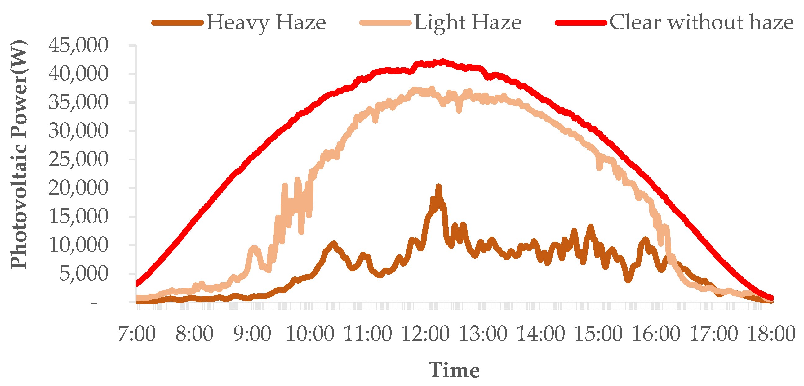
2. Analysis of the Impact of Haze on Photovoltaic Power
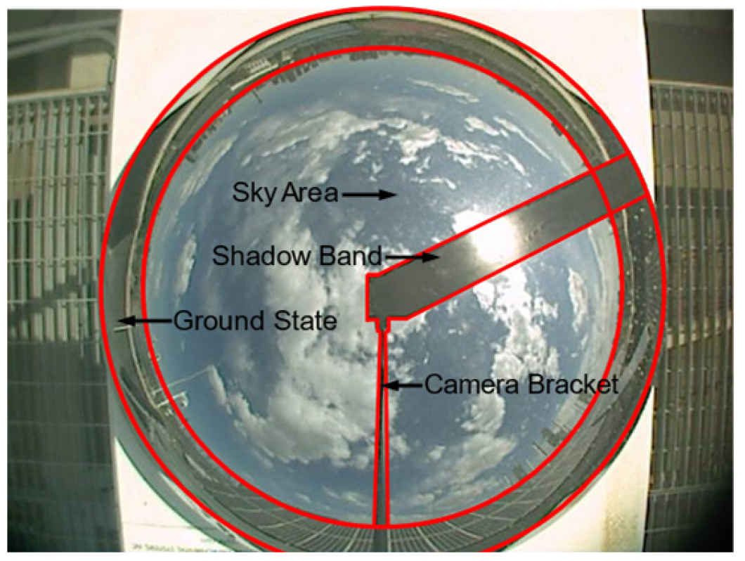
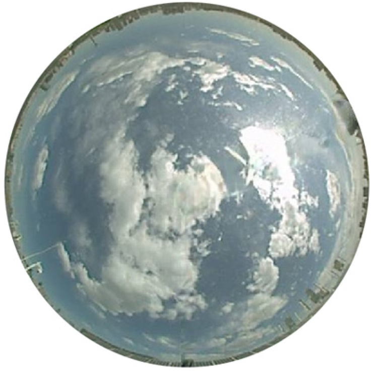
3. Ground-Based Cloud Image Introduction
4. Feature Extraction
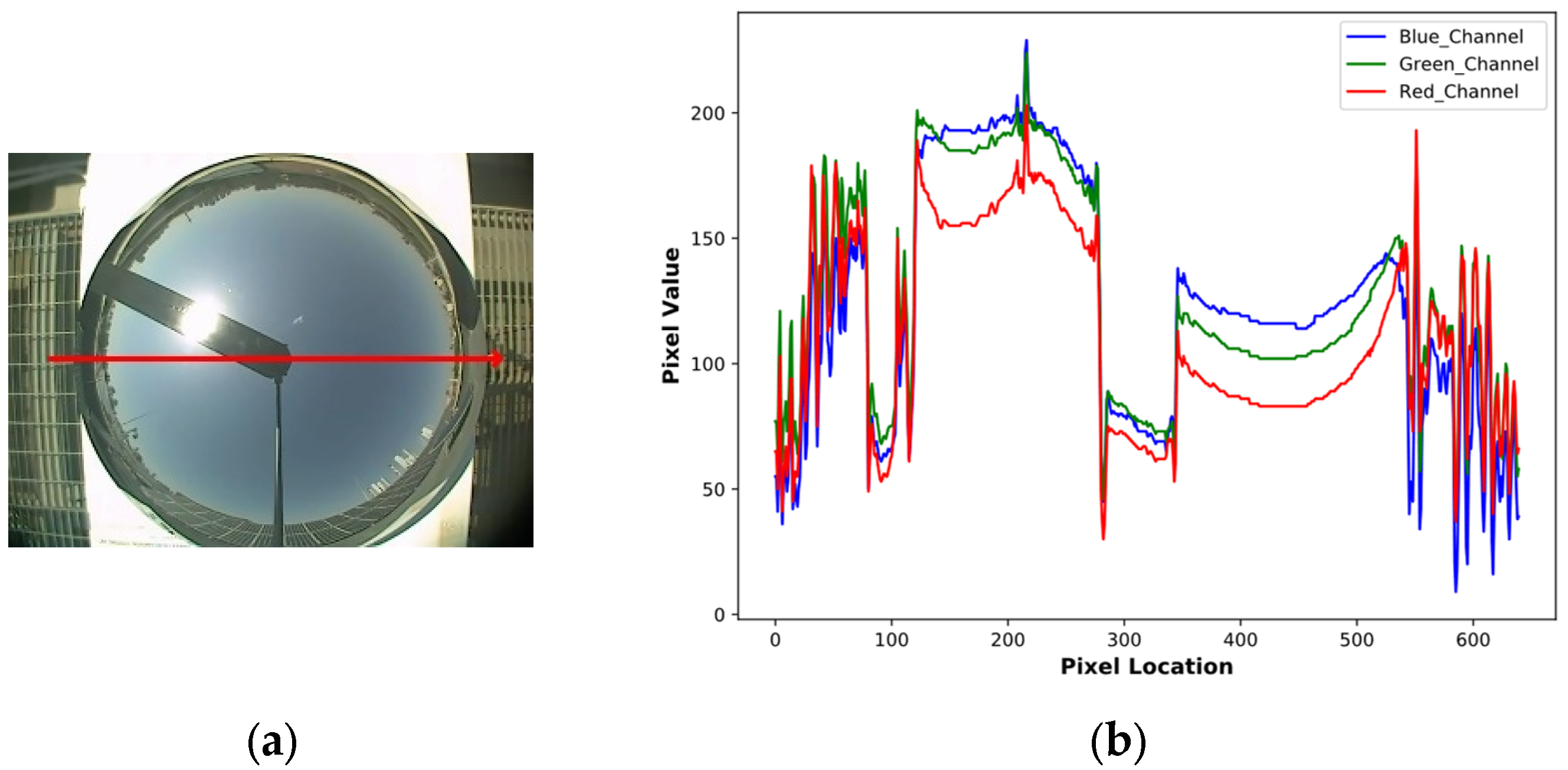
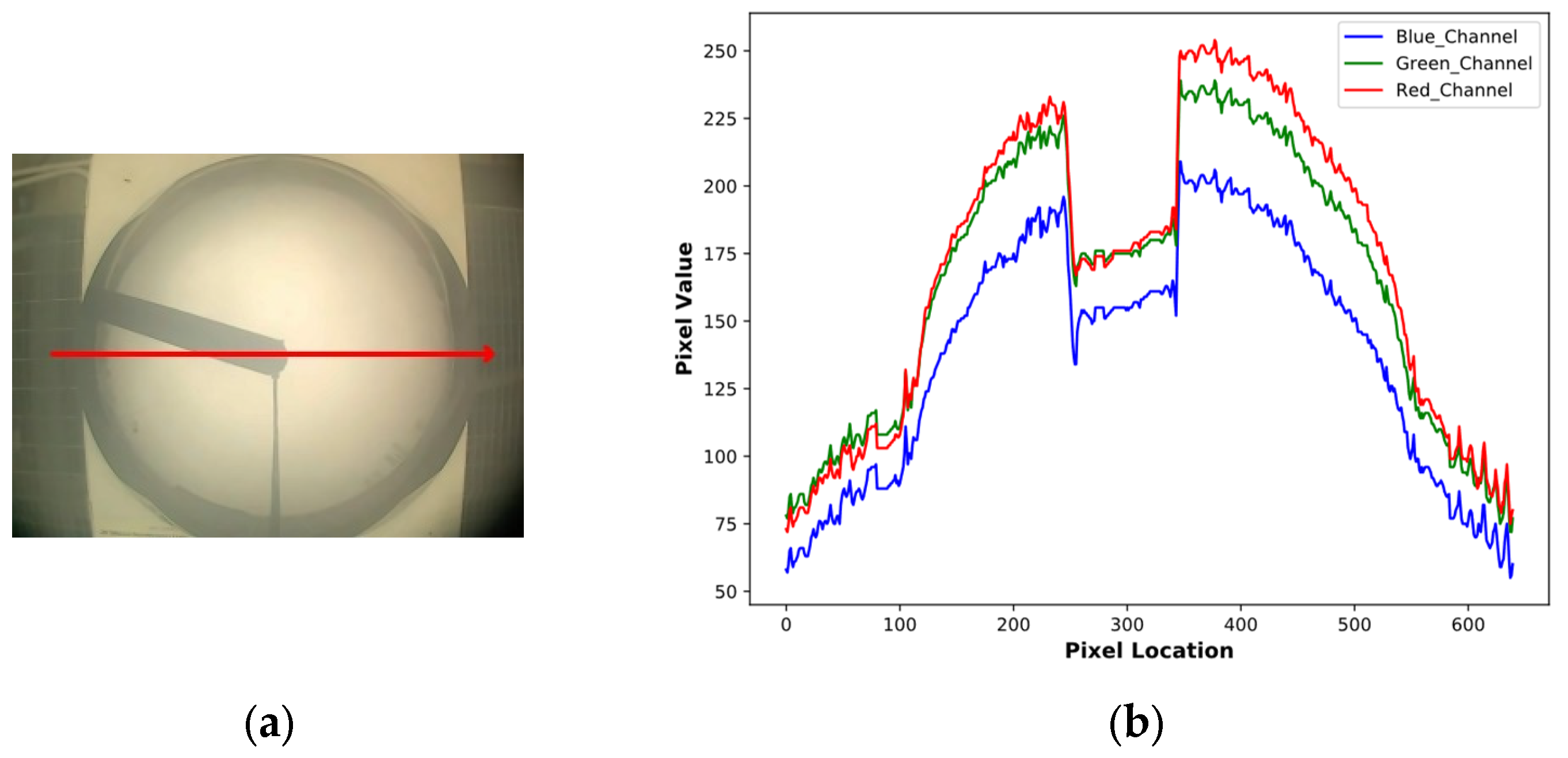
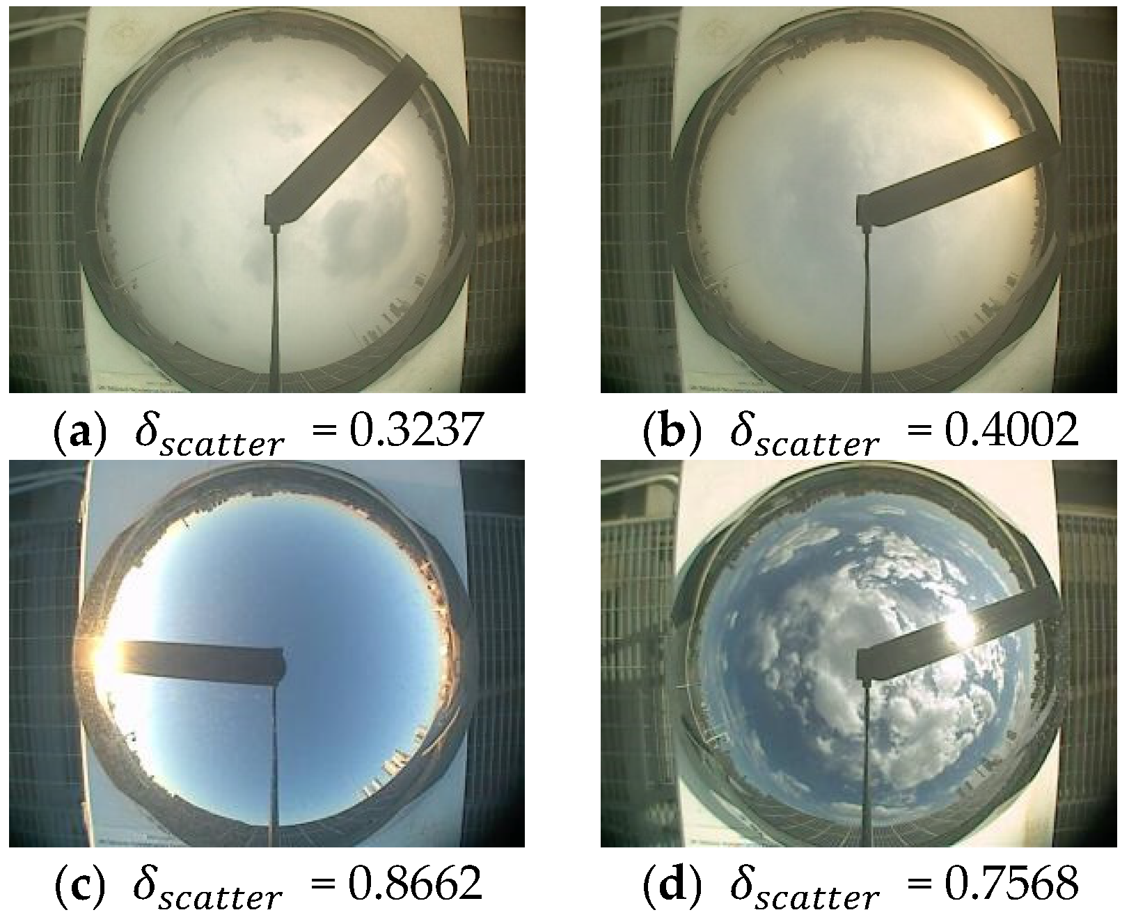
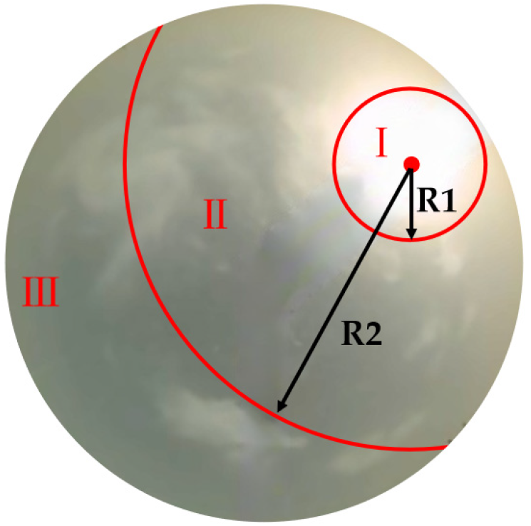
4.1. Aerosol Scattering Coefficient
4.2. Other Features
4.2.1. Cloud Cover
4.2.2. Color Features
4.2.3. Light Intensity
4.2.4. Texture Features
5. Construction and Evaluation of the Predictive Model
5.1. Model Selection
5.2. Evaluation Indices
6. Case Study
6.1. Data Preprocessing
6.2. Feature Correlation Analysis
6.3. Model Hyperparameter Tuning
- (1)
- LSTM
- (2)
- SVM
- (3)
- XGBoost
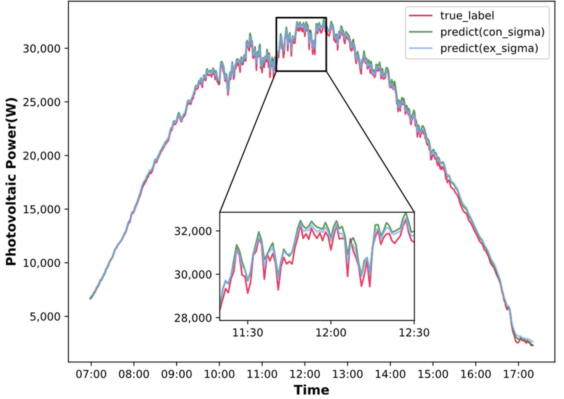
6.4. Forecast Results
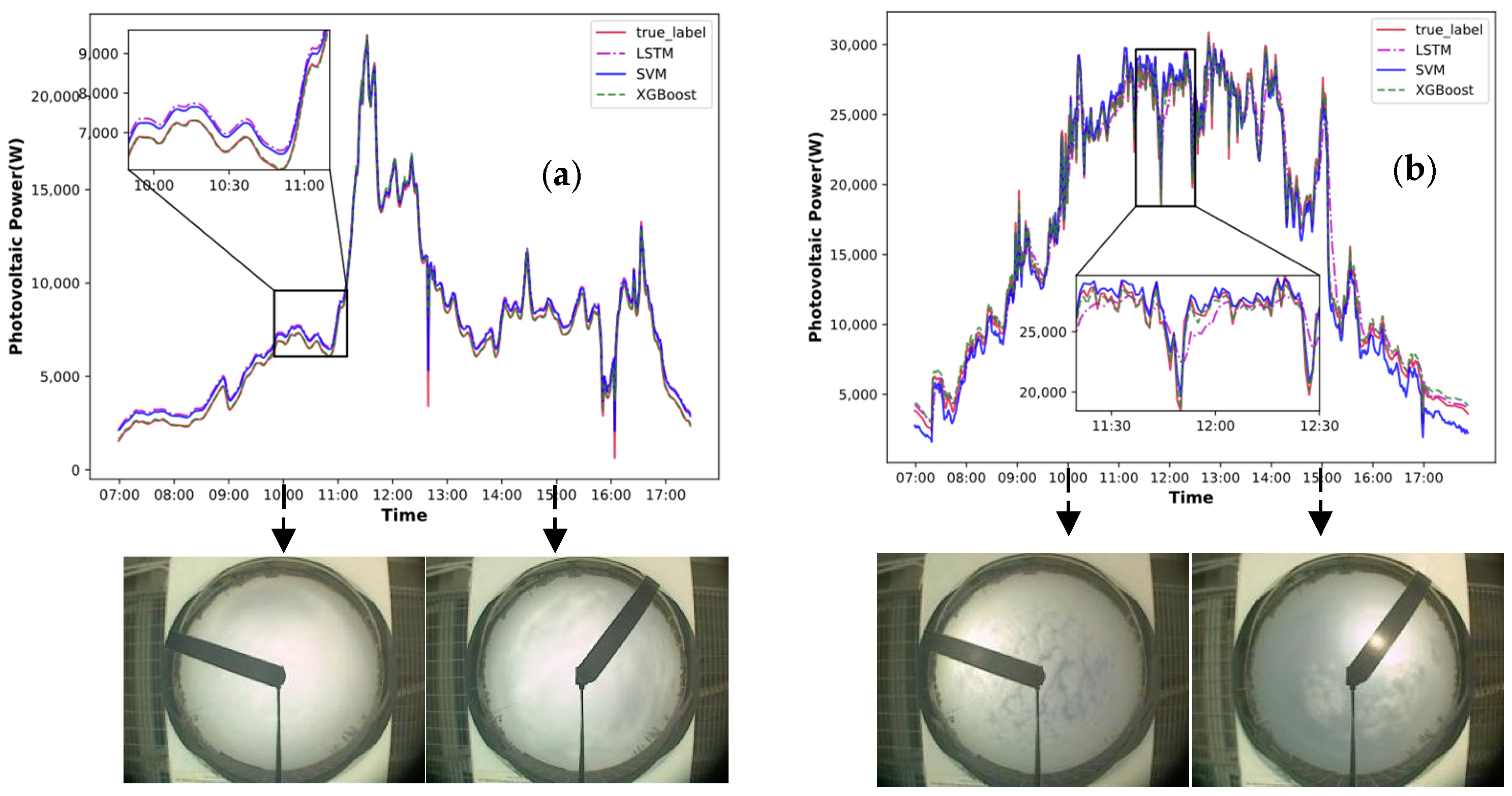
6.4.1. Prediction Results of Photovoltaic Power in Haze Weather
6.4.2. The Effect of the Scattering Coefficient Feature on the Prediction Results
- (1)
- Case of Haze Weather

- (2)
- Case of Clear Weather
7. Conclusions
Author Contributions
Funding
Institutional Review Board Statement
Informed Consent Statement
Data Availability Statement
Acknowledgments
Conflicts of Interest
References
- Mohamad Radzi, P.N.L.; Akhter, M.N.; Mekhilef, S.; Mohamed Shah, N. Review on the Application of Photovoltaic Forecasting Using Machine Learning for Very Short- to Long-Term Forecasting. Sustainability 2023, 15, 2942. [Google Scholar] [CrossRef]
- Seyyed, A.S.; Bram, H.; Joshua, M.P. A Review of the Effects of Haze on Solar Photovoltaic Performance. Renew. Sustain. Energy Rev. 2021, 167, 112796. [Google Scholar]
- Rahim, N.A.; Mohammed, M.F.; Eid, B.M. Assessment of effect of haze on photovoltaic systems in Malaysia due to open burning in Sumatra. IET Renew. Power Gene 2016, 11, 299–304. [Google Scholar] [CrossRef]
- Neher, I.; Buchmann, T.; Crewell, S.; Evers-Dietze, B.; Pfeilsticker, K.; Pospichal, B.; Schirrmeister, C.; Meilinger, S. Impact of atmospheric aerosols on photovoltaic energy production Scenario for the Sahel zone. Energy Procedia 2017, 125, 170–179. [Google Scholar] [CrossRef]
- Gutiérrez, C.; Somot, S.; Nabat, P.; Mallet, M.; Gaertner, M.Á.; Perpiñán, O. Impact of aerosols on the spatiotemporal variability of photovoltaic energy production in the Euro-Mediterranean area. Sol. Energy 2018, 174, 1142–1152. [Google Scholar] [CrossRef]
- Chu, H.Y.; Gao, Z.Q.; Sheng, S.Q. Photovoltaic power prediction method considering the influence of haze. Hebei Electric Power Tech. 2014, 5, 23–26. [Google Scholar]
- Liu, W.; Liu, C.; Lin, Y.; Ma, L.; Xiong, F.; Li, J. Ultra-Short-Term Forecast of Photovoltaic Output Power under Fog and Haze Weather. Energies 2018, 11, 528. [Google Scholar] [CrossRef]
- Liu, J.; Wang, X.; Hao, X.D. Photovoltaic power generation power prediction based on multidimensional meteorological data and PCA-BP neural network. Power Syst. Clean Energy 2017, 33, 122–129. [Google Scholar]
- Li, Y.Q.; Du, Y.Y. Short-term prediction of photovoltaic power generation based on two-dimensional sequential filling framework and improved Kohonen weather clustering. Electr. Power Autom. Equip. 2019, 39, 60–65. [Google Scholar]
- Feng, Y.; Hao, W.; Li, H. Machine learning models to quantify and map daily global solar radiation and photovoltaic power. Renew. Sustain. Energy Rev. 2020, 118, 109393. [Google Scholar] [CrossRef]
- Park, S.U.; Joo, S.J.; Lee, I.H. The reduction of the global irradiance due to the Asian Dust Aerosols (PM 10) estimated by the observed data in the dust source region of Erdene in Mongolia. Asia-Pac. J. Atmos. Sci. 2019, 55, 459–476. [Google Scholar] [CrossRef]
- Kuo, W.C.; Chen, C.H.; Chen, S.Y.; Wang, C.C. Deep Learning Neural Networks for Short-Term PV Power Forecasting via Sky Image Method. Energies 2022, 15, 4779. [Google Scholar] [CrossRef]
- Gao, R.; Xue, M.Z.; Zhao, Z.; Sheng, W.M. Ultra-short-term solar PV power forecasting based on cloud displacement vector using multi-channel satellite and NWP data. In Proceedings of the 40th Chinese Control Conference (CCC), Shanghai, China, 26–28 July 2021; pp. 5800–5805. [Google Scholar]
- Lu, Z.; Wang, Z.; Li, X.; Zhang, J. A Method of Ground-Based Cloud Motion Predict: CCLSTM + SR-Net. Remote Sens. 2021, 13, 3876. [Google Scholar] [CrossRef]
- Yang, H.; Kurtz, B.; Nguyen, D. Solar irradiance forecasting using a ground-based sky imager developed at UC San Diego. Solar Energy 2014, 103, 502–524. [Google Scholar] [CrossRef]
- Catalina, A.; Alaiz, C.M.; Dorronsoro, J.R. Combining Numerical Weather Predictions and Satellite Data for PV Energy Nowcasting. IEEE Trans. Sustain. Energy 2020, 11, 1930–1937. [Google Scholar] [CrossRef]
- Kansal, I.; Kasana, S.S. Improved color attenuation prior based image de-fogging technique. Multimed. Tools Appl. 2020, 79, 12069–12091. [Google Scholar] [CrossRef]
- Kansal, I.; Kasana, S.S. Weighted image de-fogging using luminance dark prior. J. Mod. Opt. 2017, 64, 2023–2034. [Google Scholar] [CrossRef]
- Zhen, Z.; Wang, F.; Sun, Y.; Mi, Z.; Liu, C.; Wang, B.; Lu, J. SVM based cloud classification model using total sky images for PV power forecasting. In Proceedings of the 2015 IEEE Power & Energy Society Innovative Smart Grid Technologies Conference (ISGT), Washington, DC, USA, 18–20 February 2015; pp. 1–5. [Google Scholar]
- Lu, Z.; Zhou, Z.; Li, X.; Zhang, J. STANet: A Novel Predictive Neural Network for Ground-Based Remote Sensing Cloud Image Sequence Extrapolation. IEEE Trans Geos. Remote Sens. 2023, 61, 1–11. [Google Scholar] [CrossRef]
- Kamadinata, J.O.; Tan, L.K.; Suwa, T. Sky image-based solar irradiance prediction methodologies using artificial neural networks. Renew. Energy 2019, 134, 837–845. [Google Scholar] [CrossRef]
- Scolari, E.; Sossan, F.; Haure, T.M. Local estimation of the global horizontal irradiance using an all-sky camera. Sol. Energy 2018, 173, 1225–1235. [Google Scholar] [CrossRef]


| Time Point | Sunny Day | Light Haze | Heavy Haze |
|---|---|---|---|
| 09:30 |  |  |  |
| 12:30 | 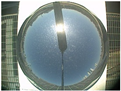 | 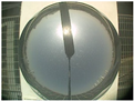 |  |
| 14:30 |  | 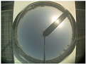 |  |
| Epoch | Number of Neurons per Layer | Batch Size | Learning Rate | Optimization Algorithm |
|---|---|---|---|---|
| 80 | [64,128] | 16 | 0.001 | Adam |
| Kernel Function | Kernel Function Coefficient | Penalty Coefficient |
|---|---|---|
| RBF | 0.1 | 1.0 |
| Epoch | Maximum Tree Depth | Random Sampling Rate | Loss Function | Learning Rate | Solve Method |
|---|---|---|---|---|---|
| 55 | 5 | 0.95 | reg:linear | 0.1 | gbtree |
| Evaluation Indices | 21 April 2021 (Heavy Haze) | 25 April 2021 (Light Haze) | ||||
|---|---|---|---|---|---|---|
| LSTM | SVM | XGBoost | LSTM | SVM | XGBoost | |
| MAPE% | 8.341 | 4.932 | 1.275 | 9.744 | 6.559 | 3.801 |
| MAE/W | 449.111 | 364.571 | 86.997 | 938.879 | 675.461 | 365.520 |
| RMSE/W | 477.899 | 392.979 | 302.179 | 1379.226 | 785.252 | 529.869 |
| 0.98630 | 0.99079 | 0.99492 | 0.97460 | 0.99307 | 0.99754 | |
| Evaluation Indices | [21] | [22] | Ours |
|---|---|---|---|
| MAPE% | 11.81 | 8.94 | 6.39 |
| % | 11.75 | 9.24 | 4.58 |
| 0.95217 | 0.96345 | 0.98694 |
| Evaluation Indices | Heavy Haze | Light Haze | Cloudy Day | |||
|---|---|---|---|---|---|---|
| MAPE% | 1.275 | 14.839 | 3.801 | 5.244 | 3.271 | 3.084 |
| MAE/W | 86.997 | 429.147 | 365.520 | 598.827 | 380.817 | 398.342 |
| RMSE/W | 302.179 | 545.028 | 529.869 | 831.631 | 504.330 | 503.211 |
| 0.99492 | 0.98409 | 0.99754 | 0.99155 | 0.99663 | 0.9967 | |
Disclaimer/Publisher’s Note: The statements, opinions and data contained in all publications are solely those of the individual author(s) and contributor(s) and not of MDPI and/or the editor(s). MDPI and/or the editor(s) disclaim responsibility for any injury to people or property resulting from any ideas, methods, instructions or products referred to in the content. |
© 2023 by the authors. Licensee MDPI, Basel, Switzerland. This article is an open access article distributed under the terms and conditions of the Creative Commons Attribution (CC BY) license (https://creativecommons.org/licenses/by/4.0/).
Share and Cite
Lu, Z.; Chen, W.; Yan, Q.; Li, X.; Nie, B. Photovoltaic Power Forecasting Approach Based on Ground-Based Cloud Images in Hazy Weather. Sustainability 2023, 15, 16233. https://doi.org/10.3390/su152316233
Lu Z, Chen W, Yan Q, Li X, Nie B. Photovoltaic Power Forecasting Approach Based on Ground-Based Cloud Images in Hazy Weather. Sustainability. 2023; 15(23):16233. https://doi.org/10.3390/su152316233
Chicago/Turabian StyleLu, Zhiying, Wenpeng Chen, Qin Yan, Xin Li, and Bing Nie. 2023. "Photovoltaic Power Forecasting Approach Based on Ground-Based Cloud Images in Hazy Weather" Sustainability 15, no. 23: 16233. https://doi.org/10.3390/su152316233
APA StyleLu, Z., Chen, W., Yan, Q., Li, X., & Nie, B. (2023). Photovoltaic Power Forecasting Approach Based on Ground-Based Cloud Images in Hazy Weather. Sustainability, 15(23), 16233. https://doi.org/10.3390/su152316233