Modeling Chlorine Decay in Reclaimed Water Distribution Systems—A Lisbon Area Case Study

Abstract

Climate change has emerged as a global challenge, with consequences for the environment and societies. To mitigate its impacts, reclaimed water (RW) offers potential by reducing water withdrawal and minimizing pollution discharges in the environment. Safe RW requires disinfection and a sound management of chlorine residuals throughout the RW distribution systems (RWDSs). This study focuses on implementing and calibrating a chlorine decay model using EPANET-MSX in a real RWDS, incorporating both bulk and wall decays. The bulk decay accounts for reactions of monochloramine formation, auto-decomposition, and depletion by a parallel second-order mechanism where monochloramine reacts both with fast and slow organic matter reactive fractions. Two wall decays were considered in the RWDS, one in the tank, modeled through an overall wall decay constant, and one in the pipes, modeled through a wall decay constant. Field experiments were conducted to calibrate the complete model. This model was used as a support tool to diagnose the RWDS status condition and cleaning needs, and to manage its operation. Through simulated scenarios considering monochloramine wall decays similar to those observed in drinking water distribution systems, the model allowed predicting adequate chlorine dosing in summer and winter scenarios, so as to guarantee monochloramine concentrations between 1 mg/L and 5 mg/L through the network. These results point to the potential use of much lower doses than the ones currently applied.

1. Introduction

Climate change has emerged as a defining global challenge, exerting profound impacts on the environment and human societies. Among its many consequences, altered precipitation patterns, floods, rising temperatures, and increased water scarcity pose significant challenges for the sustainable management of water resources. In this context, the use of reclaimed water (RW) has gained prominence as a viable solution to address both water scarcity and the growing demand for freshwater resources. The use of RW can minimize the freshwater withdrawal and the discharges and pollution in the receiving environment.

The European Union (EU), as a leading proponent of sustainable water management, has recently revised its directive (Directive 91/271/EEC) [1] on urban wastewater treatment (UWWTD). The UWWTD aims to ensure that countries properly collect, treat, and discharge wastewater, protecting the environment from the adverse effects of urban and industrial wastewater discharges. Its revision [2] (under approval by the EU parliament) reflects current concerns related to urban water services’ sustainability and environmental preservation. Regarding the latter, it proposes mandatory urban wastewater collecting systems extended to all agglomerations with 1000 inhabitants or more (and not the previously legislated above 2000 inhabitants); the overall reduction in water pollution, imposing more stringent limit values to treat nitrogen and phosphorus; and additional quaternary treatment to comply with more stringent limits for micro-pollutants, namely, pharmaceuticals and microplastics. It also proposes the reduction in pollution due to rain waters in large agglomerations, which will require the implementation of integrated urban water management plans (the use of constructed wetlands, among other nature-based solutions, is seen as an attractive method for overflow treatment in Mediterranean urban areas [3]). As for sustainability, it calls for energy neutrality and circular economy, namely, to systematically consider water reuse.

To implement these requirements, improvements in urban drainage systems and upgrades in treatment processes are foreseen, leading to an increase in the availability of high-quality treated wastewater, which may contribute to the promotion of alternative water sources. Wastewater treated to the appropriate quality standards will offer an even more sustainable and reliable source of RW, which can be used for urban irrigation and cleaning, agriculture, and industrial processes.

The European regulation on the minimum requirements for water reuse for agriculture irrigation published in 2020 [4] sets quality standards and guidelines for the treatment and distribution of reclaimed water, reinforcing the guidelines for treated wastewater use for irrigation ISO 16075-2:2020 [5]. The main similarities are the categories of treated wastewater and the suggestion to monitor RW quality parameters, such as BOD, TSS, turbidity, and biological parameters. However, ISO 16075 2:2020 [5] is more objective regarding residual chlorine dosages to maintain the RW quality for irrigation. When the category of the treated water is above “Good quality”, the thermo-tolerant coliforms need to be monitored [5]. A disinfection method is suggested to be used and a residual chlorine dosage between 0.2 mg/L and 1 mg/L measured after 30 min of contact time can be necessary for high and very high RW quality [5].

However, concerns have been raised regarding the preservation of disinfected effluents from the Water Resource Recovery Facility (WRRF) where it is produced to the point of use. More studies are required on RW disinfection, promoting the efficient RW quality control and operation of reclaimed water distribution systems (RWDSs) [6].

RW disinfection with sodium hypochlorite (chlorine) is widely used due to its effectiveness, cost-efficiency, and ability to maintain a residual of free chlorine or combined chlorine in the networks. The combined chlorine can be applied directly as chloramines or can result from the application of sodium hypochlorite in RWs containing ammonia, where chloramines (mostly monochloramine) are immediately formed from the reaction of chlorine with ammonia [7].

In general, all countries require continuous monitoring of residual chlorine, although legislation defining the required concentrations has only been identified in the USA and China. In the USA [8], the required chlorine residuals and disinfection contact times differ substantially from state to state, ranging from 1 to 5 mg/L and 15 to 90 min at peak flow, respectively. Moreover, a total residual chlorine of 0.5 mg/L is indicated as a critical low limit. In China, the GB/T_18920-2020 standard [9] indicates that the chlorine concentration should exceed 1 mg-Cl₂/L after 30 min retention in chlorine contact tanks, and 0.2 mg-Cl₂/L at the outlet of pipe networks. In Australia, a range from 0.2 to 5 mg/L of free chlorine after a 30 min contact time [10] is indicated. Regarding the irrigation of green spaces or crops, the water reuse guidelines from the USEPA [8] indicate that chlorine at concentrations greater than 5 mg/L can cause severe damage to most plants. Additionally, the WateReuse Foundation [11] indicates a recommended limit of 1 mg/L of free chlorine in RW for agriculture irrigation. In Australia, it is considered that a range from 1 to 5 mg/L of chloramine or free chlorine poses a low risk to crops (not highly sensitive) and that a total chlorine residual should generally be at least 0.5 mg/L [12]. References regarding potable water disinfection can also serve as a basis for selecting a range of residual monochloramine concentration in reclaimed water. In Australia, a monochloramine residual higher than 2 mg/L or a free chlorine residual interval from 0.2 to 0.5 mg/L in the distribution networks is indicated [13]. WHO [14] and the Australian [13] guidelines for drinking water quality mention a maximum of 3 mg/L of residual monochloramine, while US EPA [15] mentions a maximum of 4 mg/L. Notably, in Portugal, the Decree-Law 119/2019 [16], relative to reclaimed water production and use, does not mention either free chlorine or combined chlorine residual values, whereas the legal requirements for drinking water [17] mention only a recommended range of free-chlorine residual in the distribution (0.2–0.6 mg/L).

Modeling chlorine decay in RWDSs is a challenging task, as it relies on the accuracy of hydraulic models to describe flows and flow velocities and on the adequacy of chlorine decay kinetic models. Mathematical models that describe the temporal and spatial variations of the hydraulics and the chlorine decay in RW are useful to predict and analyze the distribution of the disinfectant in RWDSs. There are several software programs available to model water distribution networks, which incorporate mathematical models combining the laws of physics of the networks with the pressure and flow equations related to the operational elements. The most popular is EPANET, from US EPA, a free and opensource software that is the basis for other models, such as WaterGEMS from Bentley, Mike+ from DHI, and InfoWorks WS Pro from Innovyze. Water quality modeling is connected to hydraulic modeling by water age (residence time) and is typically limited to tracking the transport and presence of just a single chemical species. To expand the capabilities of modeling multiple chemical species, a multi-species package, freeware, was created by US EPA. EPANET-MSX is one example of a free software that can support RW decay models implementation in full-scale case-studies to model any system of multiple interacting chemical species in the water [18]. Moreover, this package has been integrated in commercial software, such as MATLAB, WaterGEMS and Mike+.

This paper presents the implementation and calibration of a chlorine decay model, including chlorine bulk decay and wall decay, applied to a real RWDS using EPANET-MSX. This study is conducted to comprehensively elucidate the main steps to implement a chlorine decay model in a real RWDS, which will help to support the establishment of monitoring and operation strategies. Moreover, research on this field contributes to the use of chlorine decay models in RWDSs and to predict chlorine residuals with the necessary accuracy for a range of operational conditions.

2. Model Development

Chlorine decay has two components: decay due to reactions of chlorine with bulk water and decay due to chlorine reactions with the pipe wall material or biofilm. As such, modeling chlorine decay in RWDSs entails the setting up of the hydraulic model and the chlorine bulk decay model, leading to the integration of the chlorine wall decay reactions.

The hydraulic model presented in this paper was built in an .inp file and calibrated using EPANET. It was set up based on the characteristics of each infrastructure component (pipe lengths, material, and diameters; node elevation), RW production data, system operational conditions, and flow measurements data, and was provided and calibrated by the project designer. The hydraulic model was integrated with the chlorine decay model using EPANET-MSX, which allows for the setup of a .msx file where the chlorine decay model includes chlorine bulk decay and wall reactions.

Chlorine bulk decay models were first developed for drinking water, having evolved from simple to more complex equations involving the reactions between chlorine and the reactants [19]. The first-order model is the simplest chlorine decay model, which assumes that chlorine bulk decay rates depend only on the chlorine concentration and considers the other reactants to be in excess. However, most chlorine reactions with organic matter have been described with second-order kinetics models [19,20], in which case the decay rates depend on the concentrations of chlorine and reactants. Furthermore, the second-order parallel model has been of particular interest [21,22], as it assumes that chlorine reactions with organic matter present two chlorine decay phases, comprising an initial fast decay due to chlorine reactions with a readily oxidable fraction of organic matter (OM) and a slower decay phase due to the reaction with an OM fraction less oxidable. The model parameters to be estimated correspond to the reaction rate constants and the initial fictive organic matter concentrations related to each phase.

Most of the reported chlorine decay models were developed and tested in drinking water produced from surface water sources [21,22,23,24,25,26] (among others), whereas few studies were found for RW [6,7,27,28]. For RW, where the presence of ammonia and OM is expected, Costa et al. [7] proposed the integration of the monochloramine auto-decomposition model from Vikesland et al. [24] with a mechanism that represents the chlorine bulk decay due to reaction of OM with chlorine. Costa et al. [7] identified a parallel second-order mechanism—where monochloramine reacts both with fast and slow organic matter reactive fractions—as the most suitable mechanism for the RWs studied. The model and this mechanism are presented in

Table 1. Reactional scheme for chlorine decay in RW from Costa et al. [7], including monochloramine auto-decomposition (R1-R14; adapted from Vikesland et al. [24]) and monochloramine decay due to OM (R15-R16) and the respective reactions rates and equilibrium coefficients ¹.

	Reaction	Reaction Coefficients/Equilibrium Constants at 25 °C
R1	$\mathrm{H}\mathrm{O}\mathrm{C}\mathrm{l}+\mathrm{N}{\mathrm{H}}_3\to \mathrm{N}{\mathrm{H}}_2\mathrm{C}\mathrm{l}+{\mathrm{H}}_2\mathrm{O}$	$\mathrm{k}1=1.5\times {10}^{10}{\mathrm{M}}^{-1}{\mathrm{h}}^{-1}$
R2	$\mathrm{N}{\mathrm{H}}_2\mathrm{C}\mathrm{l}+{\mathrm{H}}_2\mathrm{O}\to \mathrm{H}\mathrm{O}\mathrm{C}\mathrm{l}+\mathrm{N}{\mathrm{H}}_3$	$\mathrm{k}2=7.6\times {10}^{-2}{\mathrm{h}}^{-1}$
R3	$\mathrm{H}\mathrm{O}\mathrm{C}\mathrm{l}+\mathrm{N}{\mathrm{H}}_2\mathrm{C}\mathrm{l}\to \mathrm{N}\mathrm{H}\mathrm{C}{\mathrm{l}}_2+{\mathrm{H}}_2\mathrm{O}$	$\mathrm{k}3=1.0\times {10}^6{\mathrm{M}}^{-1}{\mathrm{h}}^{-1}$
R4	$\mathrm{N}\mathrm{H}\mathrm{C}{\mathrm{l}}_2+{\mathrm{H}}_2\mathrm{O}\to \mathrm{H}\mathrm{O}\mathrm{C}\mathrm{l}+\mathrm{N}{\mathrm{H}}_2\mathrm{C}\mathrm{l}$	$\mathrm{k}4=2.3\times {10}^{-3}{\mathrm{h}}^{-1}$
R5	$\mathrm{N}{\mathrm{H}}_2\mathrm{C}\mathrm{l}+\mathrm{N}{\mathrm{H}}_2\mathrm{C}\mathrm{l}\to \mathrm{N}\mathrm{H}\mathrm{C}{\mathrm{l}}_2+\mathrm{N}{\mathrm{H}}_3$	$\mathrm{k}5={\mathrm{k}5}_{\mathrm{H}}\left[{\mathrm{H}}^{+}\right]+{\mathrm{k}5}_{\mathrm{H}\mathrm{C}{\mathrm{O}}_3^{-}}\left[\mathrm{H}\mathrm{C}{\mathrm{O}}_3^{-}\right]+{\mathrm{k}5}_{{\mathrm{H}}_2\mathrm{C}{\mathrm{O}}_3}\left[{\mathrm{H}}_2\mathrm{C}{\mathrm{O}}_3\right]$
R6	$\mathrm{N}\mathrm{H}\mathrm{C}{\mathrm{l}}_2+\mathrm{N}{\mathrm{H}}_3\to \mathrm{N}{\mathrm{H}}_2\mathrm{C}\mathrm{l}+\mathrm{N}{\mathrm{H}}_2\mathrm{C}\mathrm{l}$	$\mathrm{k}6=2.2\times {10}^8$ ${\mathrm{M}}^{-2}{\mathrm{h}}^{-1}$
R7	$\mathrm{N}\mathrm{H}\mathrm{C}{\mathrm{l}}_2+{\mathrm{H}}_2\mathrm{O}\to \mathrm{I}$	$\mathrm{k}7=4\times {10}^5{\mathrm{M}}^{-1}{\mathrm{h}}^{-1}$
R8	$\mathrm{I}+\mathrm{N}\mathrm{H}\mathrm{C}{\mathrm{l}}_2\to \mathrm{H}\mathrm{O}\mathrm{C}\mathrm{l}+\mathrm{p}\mathrm{r}\mathrm{o}\mathrm{d}\mathrm{u}\mathrm{c}\mathrm{t}\mathrm{s}$	$\mathrm{k}8=1\times {10}^8$ ${\mathrm{M}}^{-1}{\mathrm{h}}^{-1}$
R9	$\mathrm{I}+\mathrm{N}{\mathrm{H}}_2\mathrm{C}\mathrm{l}\to \mathrm{p}\mathrm{r}\mathrm{o}\mathrm{d}\mathrm{u}\mathrm{c}\mathrm{t}\mathrm{s}$	$\mathrm{k}9=3\times {10}^7$ ${\mathrm{M}}^{-1}{\mathrm{h}}^{-1}$
R10	$\mathrm{N}{\mathrm{H}}_2\mathrm{C}\mathrm{l}+\mathrm{N}\mathrm{H}\mathrm{C}{\mathrm{l}}_2\to \mathrm{p}\mathrm{r}\mathrm{o}\mathrm{d}\mathrm{u}\mathrm{c}\mathrm{t}\mathrm{s}$	$\mathrm{k}10=55$ ${\mathrm{M}}^{-1}{\mathrm{h}}^{-1}$
R11	$\mathrm{H}\mathrm{O}\mathrm{C}\mathrm{l}\leftrightarrow {\mathrm{H}}^{+}+\mathrm{O}{\mathrm{C}\mathrm{l}}^{-}$	p${\mathrm{K}}_{\mathrm{a}}=7.5$
R12	$\mathrm{N}{\mathrm{H}}_4^{+}\leftrightarrow {\mathrm{H}}^{+}+\mathrm{N}{\mathrm{H}}_3$	p${\mathrm{K}}_{\mathrm{a}}=9.3$
R13	${\mathrm{H}}_2\mathrm{C}{\mathrm{O}}_3\leftrightarrow {\mathrm{H}}^{+}+\mathrm{H}\mathrm{C}{\mathrm{O}}_3^{-}$	p${\mathrm{K}}_{\mathrm{a}}=6.3$
R14	$\mathrm{H}\mathrm{C}{\mathrm{O}}_3^{-}\leftrightarrow {\mathrm{H}}^{+}+\mathrm{C}{\mathrm{O}}_3^{2-}$	p${\mathrm{K}}_{\mathrm{a}}=10.3$
R15	$\mathrm{N}{\mathrm{H}}_2\mathrm{C}\mathrm{l}+{\mathrm{O}\mathrm{M}}_{\mathrm{f}}\to \mathrm{p}\mathrm{r}\mathrm{o}\mathrm{d}\mathrm{u}\mathrm{c}\mathrm{t}\mathrm{s}$	kfast; OMf0
R16	$\mathrm{N}{\mathrm{H}}_2\mathrm{C}\mathrm{l}+{\mathrm{O}\mathrm{M}}_{\mathrm{s}}\to \mathrm{p}\mathrm{r}\mathrm{o}\mathrm{d}\mathrm{u}\mathrm{c}\mathrm{t}\mathrm{s}$	kslow; OMs0

¹ The reaction coefficients and equilibrium constants were taken from Vikesland et al. [24]. I is an unidentified intermediate. Products may include: ${\mathrm{H}}_2, {\mathrm{H}}_2\mathrm{O}, {\mathrm{C}\mathrm{l}}^{-}, {\mathrm{H}}^{+}, \mathrm{N}{\mathrm{O}}_3^{-}$; ${\mathrm{k}5}_{\mathrm{H}}=2.5\times {10}^7 {\mathrm{M}}^{-2}{\mathrm{h}}^{-1}$; ${\mathrm{k}5}_{\mathrm{H}\mathrm{C}{\mathrm{O}}_3^{-}}=800 {\mathrm{M}}^{-2}{\mathrm{h}}^{-1}$; ${\mathrm{k}5}_{{\mathrm{H}}_2\mathrm{C}{\mathrm{O}}_3}=4\times {10}^4 {\mathrm{M}}^{-2}{\mathrm{h}}^{-1}$.

.

To assess the decrease in chlorine concentration over time and to estimate the bulk decay parameters, chlorine decay tests were conducted at the laboratory scale.

To characterize the chlorine decay in a RWDS, chlorine wall decay must be integrated with the chlorine bulk decay model. Chlorine wall decay parameters estimation requires field tests or laboratorial experiments with pipes representatives of the real systems. Chlorine wall decay in pipes was described with a first order kinetics [11], using Equation (1):

$$\frac{\mathrm{d}\mathrm{C}}{\mathrm{d}\mathrm{t}}=-\frac{4{\mathrm{k}\mathrm{w}}_{ }{\mathrm{k}\mathrm{f}}_{ }}{\mathrm{D}\left({\mathrm{k}\mathrm{w}}_{ }+{\mathrm{k}\mathrm{f}}_{ }\right)}\mathrm{C}$$

(1)

where C is the free chlorine concentration in the RW (mg/L), kw is the wall decay coefficient (m/h), kf is the mass transfer coefficient (m/h), and D is the pipe diameter (m). The chlorine wall decay rate is affected by substances emitted from or attached to the pipe wall and by the rate of chlorine transfer from bulk water to the reaction area of pipe wall. The wall decay coefficient correlates to the pipe age and material and depends on the temperature. The mass transfer coefficient is often calculated as a function of the molecular diffusivity of the reactive species and of the Sherwood number (Sh), which is a function of the Reynolds (Re) and Schmidt (Sc) numbers. Since the tank section in EPANET-MSX does not accept hydraulic variables, an overall wall decay, kwall, is used for tanks, following Equation (2):

$$\frac{\mathrm{d}\mathrm{C}}{\mathrm{d}\mathrm{t}}=-{\mathrm{k}\mathrm{w}\mathrm{a}\mathrm{l}\mathrm{l}}_{ }\mathrm{C}$$

(2)

3. Materials and Methods

3.1. Case Study Description

The case study was carried out at the RWDS coming from a WRRF located in Lisbon, which serves a catchment area, mainly urban, comprising a combined sewage network. After secondary treatment, a fraction of the treated wastewater undergoes 50 µm microfiltration and UV disinfection and is stored in a 1000 m³ tank for reuse (Figure 1), while the rest is discharged into the Tagus River. The effluent discharge limits are 25 mg/L for BOD₅ (the 5-day biochemical oxygen demand), 125 g/L for COD (chemical oxygen demand), and 35 mg/L for TSS (total suspended solids). Before reuse, a final disinfection was conducted using sodium hypochlorite. As the RW contains a considerable concentration of ammonia, chloramines (mostly monochloramine) are instantaneously formed from the reaction of chlorine with ammonia, thus constituting the residual disinfectant in the RWDS.

The RWDS, schematically presented in Figure 1, comprises an internal and an external pipeline. The external network is 5 km long, from the WRRF to the pumping station (PS), at sea level, and it is currently used for sieve cleaning. RW use for green spaces’ irrigation and street washing outside the WRRF is waiting for approval. Within the WRRF, the network comprises a pipeline for green spaces’ irrigation, treatment processes, and equipment cleaning. The original hydraulic model was already calibrated for the external network. The irrigation pipeline, inside the WRRF, was added to this hydraulic model and its calibration was carried out through the analysis of water traveling times, calculated based on a tracer study using NaCl and conductivity measurement. HDPE (high-density polyethylene) is the predominant pipe material and the average infrastructure service age is about 7 years. A pump, downstream of the reclaimed water tank, delivers the RW to the whole DS.

3.2. Reclaimed Waters Characterization

The organic and inorganic matrices of RW samples were characterized. These data were analyzed to understand and provide a rationale for the chlorine demand of the RW samples. The water quality parameters, selected in accordance with ISO 16075-2:2020 [5], were measured using standard analytical methods or other consolidated methods already described by the authors [7]: pH (SMEWW 4500-H+ B [29]), temperature, electrical conductivity (SMEWW 2510 B [29]), alkalinity (SMEWW 2320 B [29]), total hardness (SMEWW 2340 C [29]), turbidity (SMEWW 2130 B [29]), UV transmittance at 254 nm (T254) of non-filtered water samples [7], total suspended solids (SMEWW 2540 D [29]), BOD (SMEWW 5210-B [29]), COD (ISO 6060:1989 [30]), total and dissolved organic carbon (TOC and DOC, respectively) [31], UV absorbance at 254 nm (A254) and specific UV absorbance (SUVA, computed as A254/DOC*100 (L/(mg-C.m) [7], ammonia, and total nitrogen [7].

3.3. Chlorine Bulk Decay Tests

Chlorine bulk decay tests were conducted at the laboratory, following Powell et al.’s bottle test method [32], to estimate the model parameters for each field experiment (FE). Non-chlorinated (RW_FE1) and chlorinated RW samples (RW_FE2), collected at the RW tank inlet and outlet, respectively, were tested.

In RW_FE1, chlorination was conducted with two chlorine doses, namely, of 0.137 mM (10 mg/L) and 0.275 mM (20 mg/L). The concentration of the chlorinated species (free and total chlorine, monochloramine, and dichloramine) was measured at 5 min, 30 min, 1 h, 4 h, and 24 h of contact time. With RW_FE2, the chlorinated species were measured at the collection moment and after 8 h and 48 h. The details of the experimental procedure can be found in [7].

3.4. Chlorine Wall Decay Field Experiments

A field data collection program was carried out to characterize the RWDS and calibrate the hydraulic and chlorine decay models, consisting of in situ chlorine measurements at several points along the network. Two field experiments, FE1 and FE2, were developed during summer and winter, respectively. In both field experiments, the flow demand was measured in three sections. The RW production flow was measured at the outlet of the RW tank using a flowmeter linked to the WRRF’s SCADA. Two portable flowmeters were installed in the external network and in the irrigation network. Water samples were collected from five points along the network: before chlorination, at the RW tank outlet, after the tank where chlorination is performed, at two points along the irrigation network (R1 and R2), and at PS, the farthest point of the network. In each of these points, chlorine species (free chlorine, monochloramine, and total chlorine) were measured.

Chlorine wall decay reactions’ coefficients were estimated using the EPANET-MSX, based on the monochloramine concentration values measured along the RWDS during the field experiments (FE1 and FE2). Equation (1) was used to estimate the kw for the network, while for the tank an overall wall decay constant, kwall, was estimated using Equation (2). Model calibration was performed by sequentially adjusting the chlorine wall reaction rate coefficient, in the .msx file, to best fit the observed field measurements. The suitability of the wall decay coefficient was evaluated by comparing the predicted and the observed values of monochloramine concentration at the measured points. The wall decay coefficient was assumed to be constant throughout the network, as both materials and service age are identical.

4. Results and Discussion

4.1. Reclaimed Water Characteristics

Table 2. RW quality parameters of each sample.

Parameter	RW_FE1	RW_FE2
pH	7.0	7.0
Temperature (°C)	25	20
Electrical conductivity (µS/cm at 25 °C)	3660	n.a.
Alkalinity (mg-CaCO3/L)	155	n.a.
Total hardness (mg-CaCO3/L)	433	n.a.
Turbidity (NTU)	6.0	8.6
Transmittance at 254 nm, T254 (%)	49	36
TSS (mg/L)	21	18
BOD5 (mg-O2/L)	13	7
COD (mg-O2/L)	65	68
DOC (mg-C/L)	3.1	n.a.
TOC (mg-C/L)	3.8	n.a.
A254 (cm−1)	0.176	0.235
SUVA (L/(mg-C.m))	5.7	n.a.
Total nitrogen (mg/L)	35.9	35.7
Ammonia nitrogen (mg-N-NH4/L)	23.0	22.9

n.a.—not available.

presents the characterization results of the two reclaimed water samples tested.

The pH of both RW samples was neutral and the RW_FE1 alkalinity values showed the reasonable buffer capacity of the RW, hence assuring no significant pH variations during the chlorination assays. Moreover, the electrical conductivity (EC) and hardness, parameters that reflect the existence of ions in the RW, presented high values, mainly but not exclusively, due to the high concentrations of calcium and magnesium salts evidenced by the high total hardness values. Therefore, the chlorine demand is not expected to be considerably influenced by the water inorganic content since Ca²⁺ and Mg²⁺ ions are not oxidizable. RW_FE1 and RW_FE2 presented similar and relatively high (for microfiltered waters [33]) turbidity and TSS values, as well as a similar transmittance. The low BOD/COD ratio in both RWs (0.1–0.2) is consistent with an effective biological treatment upstream, yet biodegradable compounds were present, particularly in RW-FE1 compared to RW-FE2, as shown by their biochemical oxygen demand values (13 vs. 7 mg-O₂/L, respectively). The RW_FE1 results indicate most (82 %) of its organic matter is dissolved (DOC vs. TOC) and predominantly composed of hydrophobic, high molar mass organics (SUVA > 4 L/(mg-C∙m) [34]). TOC concentrations in this range are also indicative of rapidly chlorine bulk decay [35]. Overall, the RW characterization indicates these are RWs whose background matrix may interfere with chlorination, i.e., where particles can shield the chlorine access to reactive/oxidizable compounds and the hydrophobic organics may consume the applied chlorine. The ammonium content of the RW samples was similar, ca. 23 mg-N-NH4/L, which corresponds to 1.64 M of ammonia. As the reaction between ammonia and free chlorine (Cl₂) is equimolar, this means that, up to a chlorine dosing of 115 mg-Cl₂/L (1.64 M), only chloramines are formed [7].

4.2. Chlorine Bulk Decay Model Parameters’ Estimation

The chlorine bulk decay model used was developed earlier [7] and, according to the equations in Table 1, four model parameters were calculated: the chloramine bulk decay rate constants kfast and kslow and the initial fast and slow OM fictive fractions, OMf0 and OMs0, respectively. The chlorine bulk parameters were estimated using the COMSOL Multiphysics 5.5 software through the Levenberg–Marquardt optimization algorithm, which is designed specifically for solving least-squares-type problems [36].

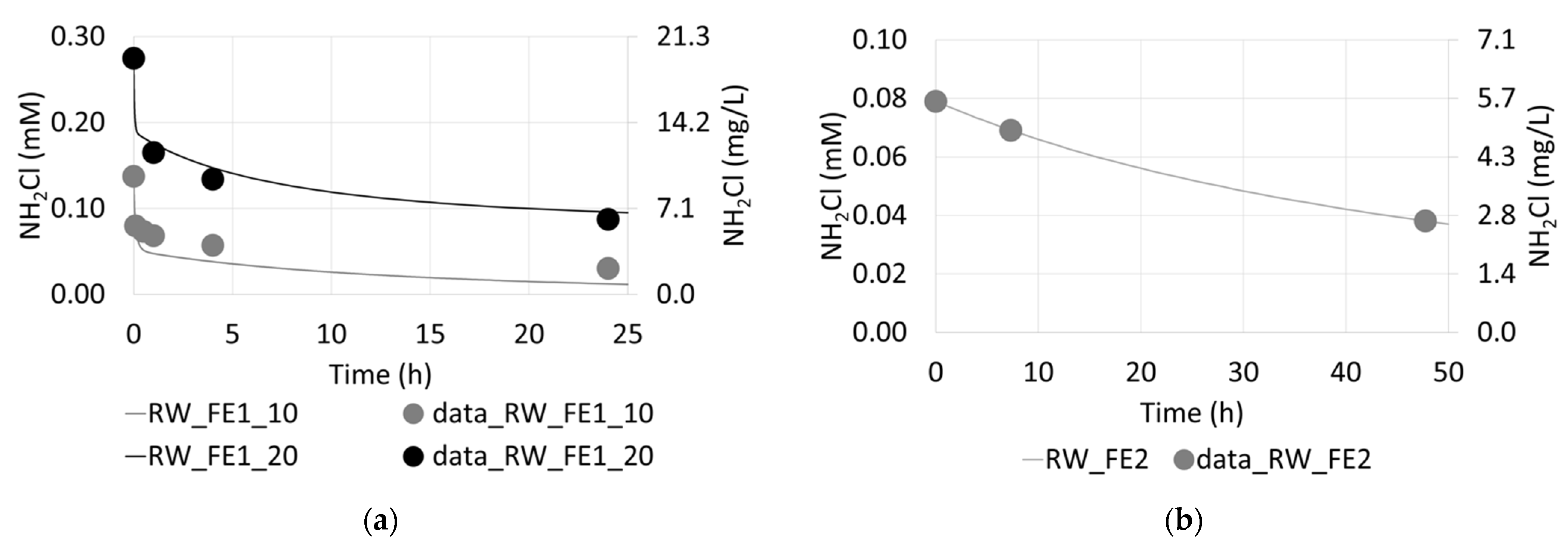
The model parameters were estimated for both field experiments, FE1 and FE2. For the non-chlorinated RW sample (RW_FE1), all reactions in the chlorine bulk decay model (R1–R16) were considered. For the chlorinated RW sample (RW_FE2), the OMf fraction was assumed to have been consumed. An initial monochloramine dose of 0.079 mM (≈6 mg/L) was measured at the time when the sample was collected. The measured and modeled monochloramine decay results are presented in Figure 2 for the RW_FE1 and RW_FE2 samples. The decay profiles in RW_FE1 clearly present two decay phases: a rapid decay during the first minutes and a long-term decrease thereafter. In the RW_FE2 case, only the slow decay of monochloramine was observed as the fast decay had already occurred during the contact time of chlorine with the effluent in the RW tank.

The modeled concentrations are fairly close to the experimental results. The high R² value of 0.95 indicates the model’s goodness of fit for RW_FE1. For RW_FE2, as expected given the low number of experimental data, the same was confirmed. The model parameters obtained for each RW are presented in

Table 3. Estimated chlorine bulk decay model parameters for RW_FE1 and RW_FE2.

	RW_FE1	RW_FE2
OMf0 (M)	1.0 × 10−4	0
OMs0 (M)	8.5 × 10−5	1.2 × 10−4
kfast (M−1h−1)	1.1 × 105	-
kslow (M−1h−1)	800	153

.

Observing the values in Table 3, the concentration of the slow-reacting organic matter with monochloramine (OMs0) is higher in RW_FE2 than in RW-FE1. However, it is expected to be less reactive than that of FE1, given the lower reaction rate constant (kslow). Comparing these values with the RW characteristics (Table 2, Section 4.1), the higher calculated OMs0 in RW_FE2 may be due to its higher contents of suspended and colloidal matter (higher turbidity) and/or of aromatic organic compounds (higher A254 values) compared to RW_FE1.

Further studies are being developed with a wider range of RWs as to better understand and correlate their characteristics with the chlorine bulk decay model parameters.

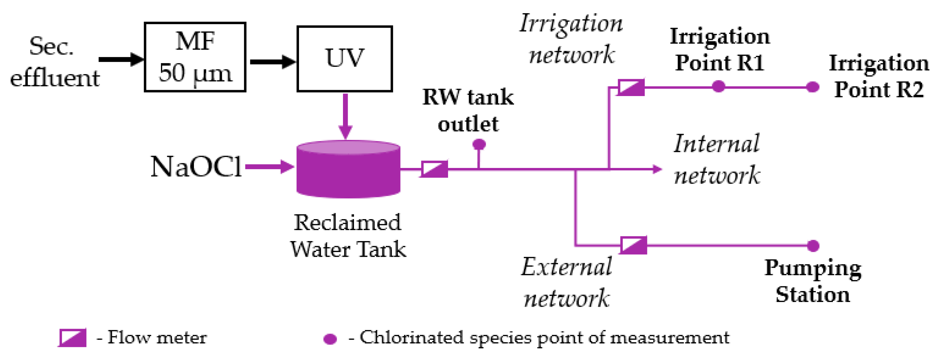
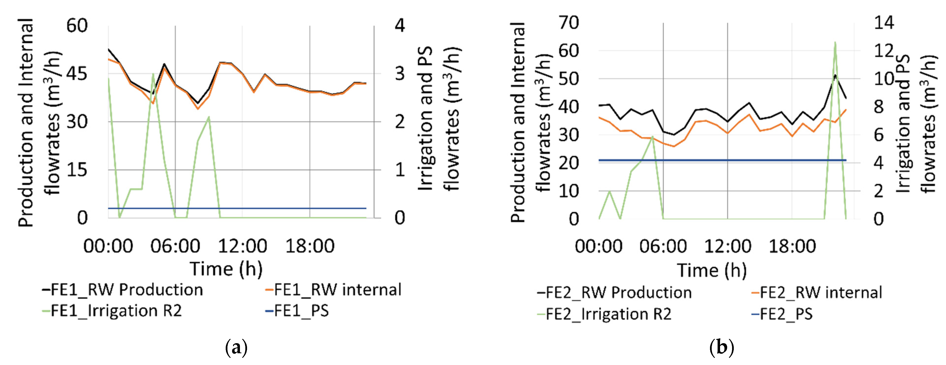
4.3. RWDS Flow Patterns

A daily flowrate pattern demand for the RWDS was established for summer and winter based on flowrate measurements (Figure 3) during the two field experiments, FE1 and FE2. The irrigation flowrate was measured in the main pipe; therefore, the total demand was added at the farthest irrigation point R2. In fact, this simplification was assumed due to the proximity between R1 and R2 and to the very similar residual chlorine concentrations observed during the field experiments.

4.4. Chlorine Wall Decay Model Parameters’ Estimation

Two field experiments were conducted, one in the summer (FE1) and one in the winter (FE2).

Table 4. Flow rate demand, initial chlorine, and monochloramine concentrations measured during FE1 and FE2.

	FE1	FE2
Flowrate demand at tank outlet (m3/h)	41.3	35.7
Flowrate demand at PS (m3/h)	0.2	4.2
Initial chlorine dosed to the RW tank (mg/L)	88	53
NH2Cl measured at the RW tank outlet (mg/L)	2.1	2.6
NH2Cl measured at R1 (mg/L)	2.1	2.6
NH2Cl measured at R2 (mg/L)	2.0	2.4
NH2Cl measured at PS (mg/L)	0.1	0.1

presents the flow demand and the initial chlorine and the monochloramine values measured during FE1 and FE2.

The total RW production, measured at the tank outlet, was quite similar in both field experiments. However, the flow demand at PS increased from 0.2 m³/h in FE1 to 4.2 m³/h in FE2. This was intentionally programmed in order to reduce the water age (hydraulic residence time) from the RW tank to the farthest point of the network, PS, and, thus, to try to achieve a higher monochloramine concentration there. The measured monochloramine concentrations at the RW tank outlet and at the irrigation points R1 and R2 (inside the WRRF) in both field experiments were similar. This indicates that the monochloramine decay to these points and among them is not significant, which was expected given the fact that these points are very close to the tank and between them (80 m distant). Moreover, at the PS node (the furthest node from the RW tank where chlorine is added, which is 5 km distant), the monochloramine concentrations were consistently lower than the chlorine concentrations at the other nodes and approximately zero.

Table 5. Tank comprehensive wall decay constant and network wall decay constant estimated values using the FE1 and FE2 data.

	FE1	FE2
kwall tank (h−1)	4	1.6
kw network (m/h)	≥0	>0.5

presents the tank overall wall decay constant and the network wall decay constant estimated for the FE1 and FE2 conditions.

Given the limited monitoring data and the gross uncertainty involved, the proposed EPANET-MSX model for the RWDS provided acceptable results for the overall wall decay constants, kwall, for tanks.

As no reference values for monochloramine wall decay were found for RW, these results were compared with those reported in Ma et al. [25] for drinking water distribution systems, 0.03–0.06 h⁻¹, which could be regarded as the minimum wall demand. The considerable higher kwall obtained in this paper for FE1 led us to conduct a thorough cleaning of the tank, which resulted in a major reduction (60%) of the tank wall demand between the field experiments.

Regarding the kw network, in both field experiments, the calculated values must be regarded as a minimum value since the measurement of chlorine decay of nearly zero could have occurred earlier. In FE1, the very low values of flow demand, which lead to a hydraulic residence time in the PS node of 7 days, which is sufficient to consume all the monochloramine present in the network, invalidated the use of hydraulic variables and the estimation of the kw network value. In FE2, the value obtained (≥0.5 m/h) was considerable higher than those reported in Ma et al. [25] for drinking water distribution systems, 0.01–0.2 m/h, indicating the potential presence of a biofilm or other deposits. Notably, the kw values obtained in this study are two orders of magnitude higher than those reported by Lee et al. [37] for free chlorine wall decay in laboratory tests with RW in PVC pipes.

To reduce or eliminate the presence of the biofilm and the consequent monochloramine decay, a network cleaning comprising a full renovation of the RW inside the pipes is recommended. To evaluate the cleaning efficacy, turbidity should be monitored during the process, with peaks of turbidity expected to occur at an initial phase. The turbidity stabilization in values below 10 NTU [8] is an indicator that the cleaning process was accomplished, allowing the beginning of the control of the disinfectant residual concentration. This simple procedure will provide information about the system condition and will contribute to the minimization of the oxidant demand.

4.5. Scenarios Simulations

Scenarios regarding the estimation of the initial chlorine doses to guarantee monochloramine concentrations between 1 mg/L and 5 mg/L (to provide a disinfectant residual without damaging the grass) at the irrigation points and PS were developed.

Two scenarios, summer (S1) and winter (S2), were proposed for the simulation of the monochloramine residual concentration using the wall decay coefficients proposed in Ma et al. [25] for drinking water distribution systems in Tianjin, China, a large looped water distribution system. kwall values (for the ideal pipe wall conditions) of 0.06 h⁻¹ (summer) and 0.03 h⁻¹ (winter) were assumed in the tanks and kw values of 0.2 m/h (summer) and 0.01 m/h (winter) were used for the network, regarded as the minimum wall demands. The scenarios were simulated using the daily flow pattern demand for the RWDS based on flow measurements during FE2. In addition, the simulations considered the minimum and the maximum daily flow demand in the network.

The minimum and maximum monochloramine residual concentrations values, for each point of analysis along the network and according to each scenario (S1 and S2), are presented in

Table 6. Estimated chlorine concentration doses and minimum and maximum monochloramine residual concentrations along the network, for scenarios S1 (summer) and S2 (winter).

	S1 (Summer)		S2 (Winter)
kwall tank (h−1)	0.06		0.03
kw network (m/h)	0.2		0.01
Initial chlorine dose (mg/L)	17		10.5
Flow demand period	Min.	Max.	Min.	Max.
NH2Cl measured at the tank outlet	4.3	4.6	2.7	2.8
NH2Cl measured at R1 and R2 (average) (mg/L)	2.1	4.3	1.7	2.7
NH2Cl measured at PS (mg/L)	1.0	1.1	1.0	1.1

.

For the summer scenario (S1), a chlorine dose of 17 mg/L allows for a monochloramine residual of approximately 5 mg/L at the RW tank outlet and ensures a minimum residual of 1.0 mg/L in the furthest point of the network. For the winter scenario (S2), with a chlorine dose of 10.5 mg/L, the minimum residual of 1.0 mg/L was achieved in the furthest point of the network, whereas a monochloramine residual of approximately 3 mg/L was provided at the RW tank outlet.

Despite the limited available data, the proposed EPANET-MSX chlorine decay model can simulate the monochloramine decay rate in the RWDS and predict the initial chlorine concentrations (to be applied) and the monochloramine residuals at the different points of the network over time. To enhance model calibration and the confidence in results, further studies should consider exploring other ranges of hydraulic residence times and increasing the number of chlorine measurements along the RWDS.

5. Conclusions

In this paper, a chlorine decay model for reclaimed water, incorporating both bulk and wall chlorine decays, was successfully implemented, calibrated, and integrated with a RWDS hydraulic model, using EPANET-MSX.

A model previously developed for RWs containing ammonia, thus promoting the formation of monochloramine, was calibrated and two wall decays were considered in the RWDS, one in the RW tank, modeled through an overall wall decay constant, and one in the pipes, modeled through a wall decay constant. Field experiments were conducted to calibrate the complete model.

Through the assessment of the hydraulic variables, in particular of the hydraulic residence time (water age), and of the calculated wall decay constants with the model, it was possible to evaluate the network management, operation, and condition, and to propose corrective measures for its improved operation and cleaning. Furthermore, the proposed model was used to conduct simulations, so as to guarantee monochloramine concentrations between 1 mg/L and 5 mg/L throughout the network, using the chlorine wall demand in chloraminated drinking water distribution systems as the reference. Summer and winter scenarios were simulated and the results point to the potential use of much lower doses than the ones currently applied.

It was shown that the integration of hydraulic models with chlorine decay models can improve the control of chlorine dosing and disinfection operations for safe reclaimed water distribution. By using a chlorine decay model, water/wastewater utilities can optimize the chlorine dose that matches the network’s properties, flow changes, and the quality standards for water reuse, thus improving the system operation without significant costs. All in all, the study shows simulation models to be indispensable management tools for understanding the behavior of systems, for establishing operational diagnoses, and for deciding on actions within the scope of planning, design, operation, and rehabilitation.

Additional studies can involve enhancing the model accuracy, using online measurements from a chlorine analyzer to establish a chlorine concentration pattern. Moreover, the use of EPANET-MSX can be made more user-friendly by using applications that enable the graphical visualization of the results. Further research can focus on estimating the parameters of the chlorine bulk decay model through the identification of correlations with RW quality parameters and improving regular updates and the real-time calibration of the models by, e.g., using online sensors. Once more knowledge is obtained, future legislation should encourage the use of modeling approaches, namely, to support chlorine dosing and the management of RWDSs.