Factors Affecting Indoor Temperature in the Case of District Heating

Abstract

In this study, the influence of variables defining indoor temperature is studied, focusing on operational data and visual and technical inspections rather than the temperature control setpoints and occupancy schedule. This is incorrect because infiltration and insolation are highly variable. This results in lowering the temperature difference between the supply and return lines, overheating some spaces, lowering the indoor temperature in others, and poor hydronic balancing. The novelty lies in studying the actual operating condition of real district heating (DH) systems. The research hypothesis is that internal heat gains along with the infiltration of and variations in outdoor temperature cause daily changes in indoor temperature. These factors seem to be the primary reasons for the variations in supply and return temperature, if the rate of energy loss is not large in new office buildings constructed according to tightened contemporary energy conservation regulations. The saving effect is achieved by allowing the energy to be dumped into building envelopes; thus, the flow rate or supply temperature are varied in a narrower range. Dumping heat by using the storage capacity of building envelopes is suggested. The corrected design approach minimizes energy consumption and increases annual performance (e.g., by 14.1% here). Advantages are achieved by tuning a controller at a DH substation.

1. Introduction

Energy storage and demand-side management are vital in the process of lowering supply temperature, which is integral to the concept of fourth-generation district heating (4GDH) [1,2]. It assumes switching to a sustainable district heating (DH) system by ensuring energy flexibility. Energy flexibility is typically defined [3] as the ability to transform the energy injection from/to energy extraction in time to avoid system limitations, which is conducive to intermittent renewable and residual energy sources. A pertinent conclusion from [4] is that, despite the energy lost through the energy accumulators, its potential is still much higher than in the case of traditional heat supply. Its main feature is heat generation, equal to the summation of the energy absorbed by various thermal masses. However, energy flexibility works another way.

There is an external temperature above which there is no need for space heating (SH); therefore, the energy demands of a building are expected to be fully dedicated to domestic hot water (DHW). Typically, this is called the control point temperature (CPT). From Ivanko et al.’s research [5], one can observe that in Europe, the CPT can be as much as 16 °C (compared with 5–8 °C in Russia [6,7]). This makes SH longer and studying factors affecting indoor temperature is even more important. Excluding weather and climate, there are a lot of such factors; for example, the behavior of consumers of a DH service (employees), indoor heating equipment, etc. Typically, these are called internal factors. Their impact has been corroborated in many studies. For instance, for all of the buildings studied by Luc et al. [8], there was a clear influence of internal heat gains. Johra et al. [9] reported the role of furniture in significantly increasing the heat inertia of new buildings. Concerning the indoor items/furniture elements, their effect is limited for highly efficient buildings, but is negligible for older ones. Additionally, the actual energy demand of a substation is constituted by the actual SH + DHW demand of the consumer and an additional amount of heat to cover distribution losses. The former depends on supply, return, and outdoor temperatures, the length of the network, etc. Last but not least, in the case of advanced SH systems, the customers together may change the SH system’s supply temperature set-point by setting a desired indoor temperature set-point profile. Additionally, some authors previously revealed that the discrepancy increases when the set points differ more from the actual values [10,11]. There are clearly visible local peaks caused by the use of DHW and the manual setting of indoor temperature during a weekday or night.

To study heat demand, Jebamalai et al. [12] inputted open-source street-level gas consumption data, which were provided by a local gas supply operator. Profiles were generated based on large datasets and considering a given typical building type in Belgium. In the present research, the difference is that the system’s total load was not only assessed by aggregating the residential energy consumption, but also by considering operational data and using profiles. Another difference concerns the DH plant, which is not assumed to have a fixed generation curve during the year.

In [13], a model of a single-family house was developed in TRNSYS. When assessing indoor temperature with the help of the TRNSYS library, the model considers the performance of envelopes and the distribution of indoor volume temperature with furniture and indoor content included. Hence, the models also consider the energy accumulated within walls and the indoor content of the zone.

Technically, the advanced control logic of newer substations enables the integration of consumers into DH network operations, involving additional active variables in the performance of the DH system. With such regulators, consumers may vary the source-side mass flow rate in the HE by changing indoor temperature set points. However, reducing the flow rate through a substation results in an increase in a DH system’s bypassing flow. Bypassing takes place on the network level. If the building substation does not extract the amount of water that was expected, all this water moves to other neighborhoods situated after that building substation along the network. Supposing there are too many such building substations: overheating occurs, which results in the high temperature of water returning to a DH plant. The side effect is an increased indoor temperature in old buildings, which do not have automated DH substations. One reason is the poor control logic of a space heating SH system; another reason is the high actual heat demand of such a building, typically being much higher than the design due to high heat losses through worn-out external envelopes (exterior walls and roof).

Compared with the present study, Sommer et al. [14] concluded that circulation pump energy remains small compared with the heat pump energy, and thus only marginally influences the seasonal pattern of total energy consumption. Nonetheless, when modeling, the electricity consumption required to run pumps is typically assumed as constant for all DH systems in any season (except for summer). The reason is the type of control of mass flow rates in distribution networks, which are assumed to be equal and constant, while the supply temperature changes.

Heat demand is the key feature of any DH system and the key component of operational data at the same time. For instance, the results from [15] pertain to the distribution and the structure of heat demand. District energy systems are considered feasible in the most populated cities in France, i.e., the 280 cities with more than 30,000 inhabitants. To ensure conversion to LTDH or 4GDH concepts, heat demand should be reduced via DSM measures. Another approach is to increase radiators’ heat area or heat transfer coefficient to keep the same amount of heat released in the case of lowering supply temperature. Taking into account that SH systems are usually slightly oversized, while the main reason for high return temperature is poor regulation, it might be sufficient to reduce the heat demand of new buildings by 10–15%. Compared with the present study, in [16], this effect could be mitigated by reducing the energy consumption in the residential sector by 16–25%.

In the study performed by Saletti et al. [17], the return temperature was lower than the statistical data, which is a reason for the surplus amount (above the design value) and the decreasing supply temperature. The main difference with our study is a full implementation of LTDH; the return temperature was fixed at the lower threshold of 30 °C. Although this is advantageous for the operation of a district energy system, it is not only highly unlikely but also unacceptable for severe climate conditions [18,19]. Hence, these conclusions are hardly valid for other locations of a DH network.

Usually [20], the heat losses through constructions are assessed by multiplication of the specific heat transfer coefficient and the area of the external envelope and indoor/outdoor temperature differences. Concerning the model and methodology, a novel linear temperature model featuring the correction factors adjusting convective heat transfer coefficients was developed. To compare data, which were input to the method, Harney et al.’s [21] paper has been studied. Similarly to this study, specifications provided for their research included the heat transfer performance of the building envelope, the total area of residential space, the area of each room, and the properties of radiators. The U-values of external surfaces of the apartment are also shown. Their limitation was that the traditional methods better matched residential buildings with low-glazing areas and limited time when entrance doors are opened.

Similarly to Fito et al. [22], economic considerations were avoided in the present study. For instance, their indicators agreed on the interest of recovering waste heat. Their values enhanced the performance of a DH system if the capacity of a thermal accumulator was increased. Even though they recommend the highest possible capacity of a heat accumulator (40 MWh), feasibility considerations may change this conclusion.

Unlike the results presented below, Quirosa et al. [23] pointed out the instantaneous heat demand covered by the DH system to follow the thermal response. They in addition this with the demand of the building and applied a similar profile to the compressor power curve. Another difference is maximization as a function of the DH supply temperature and the COP of the HP. However, for a specific winter day, the maximum value was much lower and only accounted for 44 kW.

Sun et al. [24] assessed the correction factors for substations and set them ranging from 0.80 to 1.40. The correlation between supply temperature and indoor temperature was presented as well. They reported that when the indoor temperature differed by 1 °C from the set point, the correction of supply temperature should only be 3.6–4.8 °C.

The novelty is, therefore, studying the actual operating conditions of real DH systems. The research hypothesis is that internal heat gains, in addition to the infiltration of and variations in outdoor temperature, cause daily changes in indoor temperature. These factors seem to be the primary reasons for the variations in supply and return temperature, if the rate of energy loss is not large in new office building constructed according to contemporary tightened energy conservation regulations.

Ren et al. [20] established a model for rapidly forecasting temperature fields to ensure optimal control and achieve energy saving while operating a SH system. The difference was in using Green’s function to construct a linear temperature model. Camci et al. [25] indicated a comparison of the impact of the aforementioned factors not on indoor temperature, but on the intensity of convection. They distinguished the phenomena of mixed convection and features encountered in forced convection applications. However, Camci et al. [25] calculated natural convective heat transfer coefficients using various correlations. The thermal conditions were similar, with the temperature differences ranging between 2 and 14 °C.

The global difference with our study is the inability to suggest the additional consumption of primary energy to achieve a better overall effect, but only limiting the initial values. Therefore, we do not solely follow Sun et al.’s [24], Ren et al.’s [20], or Camci et al.’s [25] ideas.

This paper suggest a new methodology for correcting design heat demand according to operational data and the inspections performed. The scope of this paper is presented in

Table 1. The summary of factors affecting the indoor temperature in the case of district heating.

	Normalized Influence		Covered by the Present Research
	Residential Building	Office Building
Primary (network) supply temperature	0.14	0.14	Yes
Secondary (space heating) supply temperature	0.23	0.23	No
Return temperature	0.08	0.08	Yes
State of the space heating system (incl. radiators)	0.17	0.15	No
Envelope state (incl. infiltration)	0.18	0.20	Yes
Thermal inertia	0.05	0.05	No
Internal heat gains	0.10	0.05	Yes
Solar insolation (incl. glazing share and building orientation)	0.05	0.10	Yes
Total	1.00	1.00	n/a

.

2. Materials and Methods

The heat consumption of a building is [W]:

Q = Q_env + Q_inf/vent − Q_in

(1)

where Q_env is the design heat demand [W], Q_inf/vent is the additional heat needed to warm cold air due to infiltration and ventilation [W], and Q_in is the heat gain [W].

Design heat demand [W]:

Q_env = U∙S∙(t_in − t_out^d),

(2)

where S is a heated area [m²] and U is the overall heat transfer coefficient (U-value) [W/(m²K)]:

$$U=\frac{\sum \frac{A_i}{R_i}}{\sum A_i}$$

(3)

where R_i is the R-value of the envelope of type i [m²K/W], A_i is the surface area of the envelope of type i [m²], t_in is the indoor temperature [K], and t_out^d is the design outdoor temperature [K].

According to modeling and inspections, Equation (2) is modified with the correction factor β to take into account the recorded difference between actual and calculated indoor temperatures to assess additional heat absorbed by surfaces after solar insolation and infiltration.

Then, heat demand compensating additional losses [W] can be calculated as follows:

Q_env + Q_inf/vent = U∙A∙(t_in − t_out^d)∙(1 + Σβ),

(4)

where β is the dimensionless correction factor [-].

For solar insolation [26]:

• β = 0.1 for indoor spaces oriented north (N), north-east (NE), north-west (NW), and east (E);
• β = −0.05 ditto, for south-east (SE) and west (W);
• β = −0.1 ditto, for south (S) and south-west (SW).

The correction factors are summarized in Figure 1.

To ensure a better understanding of infiltration processes, additional corrections to account ingress of cold air through doors [26] are applied:

• β = 0.2∙H for triple doors and two airlocks between;
• β = 0.27∙H for double doors and one airlock between;
• β = 0.34∙H for double doors without an airlock;
• β = 0.42∙H for a single door;
• β = 0.34∙H for a revolving door,

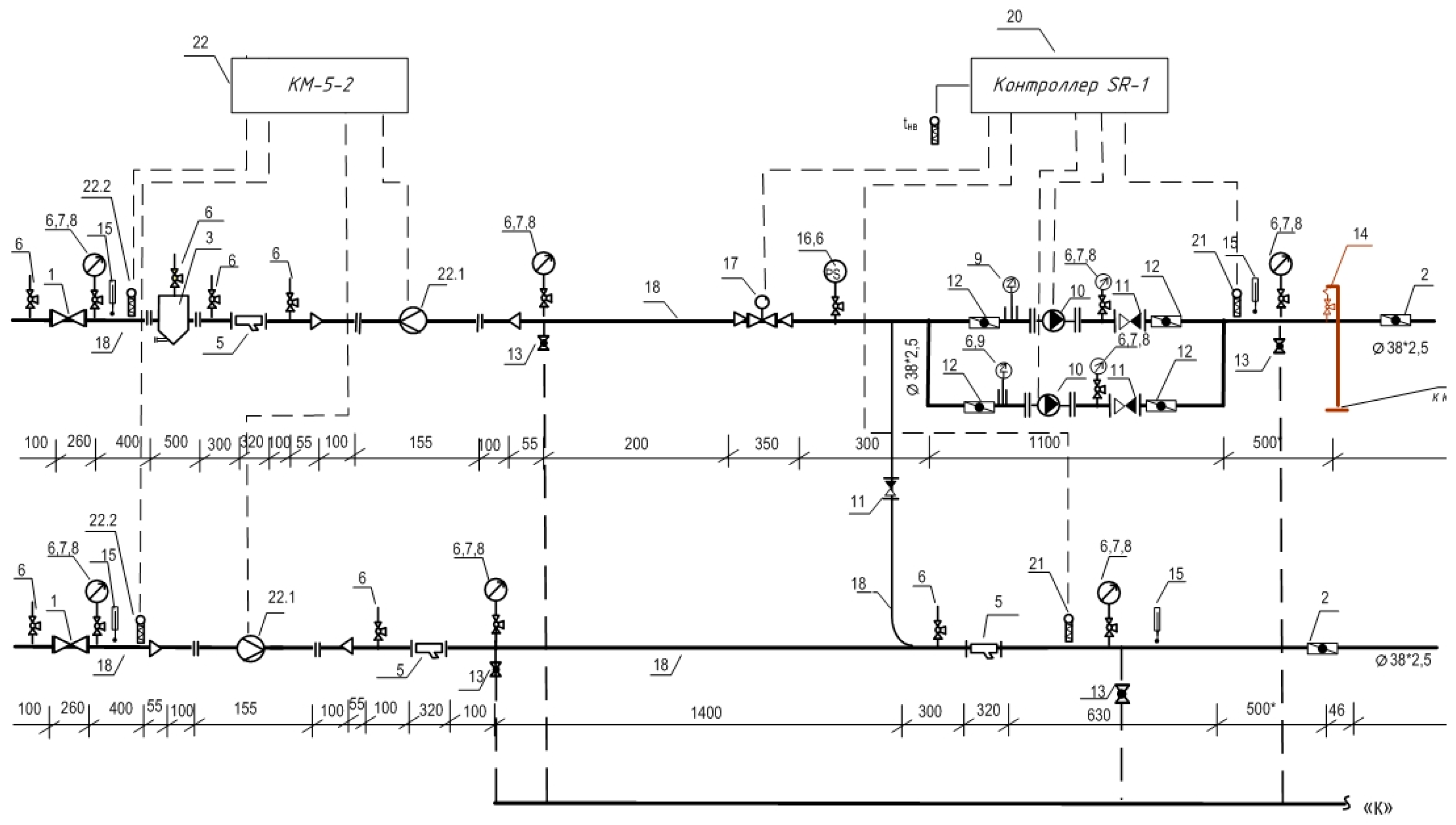
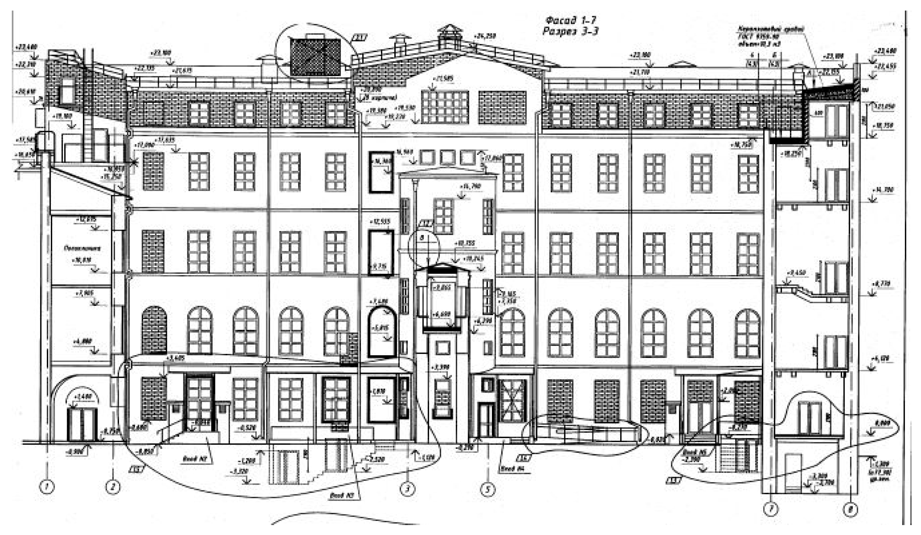
Here, H is the height of a building [m].

Additional β-values are applied to take into account the pressure difference.

Pressure difference for a specific location and terrain [Pa]:

ΔP = (H − h)∙(γ_out − γ_in) + (ρ_out∙v²/2)∙k_dyn∙(c_w − c_l) − P_in.

(5)

where h is the height of the center of a door/window/skylight [m], γ_H and γ_in are the specific weights of outdoor and indoor air, respectively [N/m³], and ρ_out is the air density of outdoor air [kg/m³]:

ρ_out = 353/(273 + t_out)

(6)

where k_dyn is a factor to take dynamic air distribution into account (depending on terrain, height, etc.), c_w are the c_l aerodynamic efficiency of a building on its windward and leeward sides, respectively (e.g., c_w = 0.8, and c_l = −0.6), and P_B is the indoor air pressure [Pa].

For well-balanced buildings:

P_B = 0.5∙H(γ_out − γ_in) + 0.25∙(ρ_out ∙v²)∙k_dyn∙(c_w − c_l),

(7)

and for poorly balanced buildings, where most of the windows are oriented to the side:

P_B = 0.5∙H∙(γ_out − γ_in) + 0.5∙ρ_out∙v²∙k_dyn∙[(c_w − c_l)∙A_w + (c_s − c_l)∙A_s]/(A_w + A_s + A_l),

(8)

where c_s is the aerodynamic efficiency of a building on its side view (e.g., c_s = −0.4), and A_w, A_s, and A_l are the door/window/skylight surface areas on the windward, side, and leeward faces, respectively [m²].

For indoor spaces with no mechanical ventilation, air intakes, or air conditioning:

P_B = (H − h)∙(γ₅ − γ_in)

(9)

where γ₅ is the specific weight of air at a temperature of +5 °C [N/m³].

SH demand profiles for a weekday and weekend day for each month during the year were obtained using the heat meter data. For a typical building, the DH substation is shown in Figure 2: when the opening of regulating valve 17 becomes smaller, the pipeline characteristic curve becomes steeper.

The result was a reduction in the flow rate at a circulation pump of a DH plant, increase in the pressure head, and divergence from the high-efficiency point. This led to a network overpressure phenomenon, affecting the hydraulic balancing of the network.

3. Case Study

To corroborate the results, the methodology was applied to one of the public buildings located in Omsk, Russia. This building now houses the State Hermitage Museum of Siberia, which is a branch of the Omsk State Art Museum named after M. A. Vrubel (Figure 3).

The R-values and design heat demand were evaluated by the sizes, orientation, and design indoor temperature (℃) in the occupied area based on the National Construction Code [27], as shown in

Table A1. Characteristics of the indoor spaces. There is one main entrance and several emergency exits on the ground- and first floors, in addition to fire escapes on the second, third, and fourth floors. Walls adjacent to the indoor spaces with colder design indoor temperature (e.g., a staircase or a vestibule) and contributing to overall heat losses are titled ‘Internal partitions’.

#	Office (Zone)	Target Indoor Temperature [°C]	Properties of Envelopes
			Wall Title (According to the Blueprints)	Orientation	Dimensions [m]	Surface Area [m2]
Ground floor
1	Tool shop	16	Internal partition #1			113.4
		16	Internal partition #2			110.4
		16	Internal partition #3			117.6
		16	Internal partition #4			181.0
		16	Window	NE	(0.6 × 1.2) × 6	4.32
		16	Door	SW	2 × 1.2	2.4
2	Storage room for household chemical goods, garage	16	Internal partition #1			135.0
		16	Internal partition #2			156.9
		16	Internal partition #3			132.2
		16	Internal partition #4			228.2
		16	Window	NE	(0.6 × 1.2) × 7	5.04
		16	Door	NW	2 × 1.2	2.4
First floor
13	Office	20	Load-bearing wall	SW	3.6 × 3.6	12.96
		20	Load-bearing wall	NW	6.6 × 3.6	23.76
12	Exhibition hall	20	Load-bearing wall	SW	18 × 3.6	47.52
		20	Window	SW	2.7 × 3.2	8.64
		20	Window	SW	2.7 × 3.2	8.64
		20	Load-bearing wall	SE	12.6 × 3.6	34.91
		20	Window	SE	2.7 × 3.87	10.45
		20	Load-bearing wall	NW	12 × 3.6	38.88
		20	Door	NE	2.4 × 1.8	4.32
		20	Load-bearing wall	NE	8 × 3.6	28.8
		20	Window	NE	1.8 × 1.77	3.19
		20	Load-bearing wall	NE	6 × 3.6	21.6
		20	Door	NW	1.8 × 2.4	4.32
		20	Window	SW	2.7 × 3.2	8.64
	Staircase/Vestibule	16	Load-bearing wall	SW	3 × 3.6	10.8
		16	Load-bearing wall	NW	7 × 3.6	26.6
		16	Load-bearing wall	NE	3 × 3.6	10.8
		16	Door	NE	1 × 2.1	2.1
2	Vestibule	20	Load-bearing wall	SW	6 × 3.6	15.36
		20	Door	SW	2.4 × 1.3	3.12
		20	Door	SW	2.4 × 1.3	3.12
3	Office	20	Window	NE	5 × 3.6	18
		20	Window	SE	5 × 3.6	18
		20	Internal partition #1		5 × 4	20
		20	Internal partition #2		2 × 3 + 2 × 0.4	6.8
		20	Internal partition #3		0.4 × 0.8	0.32
	Staircase	16	Load-bearing wall	NW	7 × 3.6	23.1
		16	Load-bearing wall	NE	4.6 × 3.6	16.56
		16	Load-bearing wall	SW	4.6 × 3.6	16.56
		16	Door	NW	1 × 2.1	2.1
4	Exhibition hall	20	Load-bearing wall	NW	6 × 3.6	21.6
		20	Load-bearing wall	SW	8 × 3.6	28.8
		20	Window	SW	3.14 × 2.7	8.5
		20	Window	SE	20 × 3.6	72
		20	Load-bearing wall	NE	21 × 3.6	75.6
		20	Door	NE	1.3 × 2.4	3.12
		20	Window	NE	1.8 × 1.8 × 4	12.96
		20	Load-bearing wall	NW	12 × 3.6	43.2
		20	Window	NW	1.8 × 1.8 × 2	6.48
		20	Door	NW	1.8 × 2.4	4.32
		20	Internal partition #1		20 × 2 + 5 × 2	50
		20	Internal partition #2		16 × 2 + 3 × 2	38
		20	Internal partition #3		18 × 1	18
Second floor
12	Office	20	Window	SW	21 × 3.75	78.75
		20	Window	NW	10 × 3.75	37.5
		20	Window	SE	10 × 3.75	37.5
	Staircase	16	Load-bearing wall	NE	7 × 3.75	22.5
		16	Window	NE	3 × 1.25	3.75
		16	Load-bearing wall	SW	3 × 3.75	11.25
		16	Load-bearing wall	NW	7 × 3.75	7.5
		16	Window	NW	3 × 1.25	3.75
6	Hallway	20	Load-bearing wall	NW	7 × 3.75	23.52
		20	Door	NW	2.1 × 1.3	2.73
		20	Load-bearing wall	NW	1.8 × 3.75	6.75
		20	Load-bearing wall	NW	1.8 × 3.75	6.75
		20	Load-bearing wall	NE	4.8 × 3.75	15.3
		20	Window	NE	0.9 × 1.5 × 2	2.7
		20	Load-bearing wall	SE	2.6 × 3.75	7.95
		20	Window	NW	1.2 × 1.5	1.8
11	Office	20	Window	SW	6 × 3.75	22.5
19	Office	20	Load-bearing wall	NE	4 × 3.75	15.0
		20	Window	NE	1.2 × 1.5	1.8
		20	Load-bearing wall	NW	6 × 3.75	22.5
		20	Window	NW	1.2 × 1.5	1.8
1	Office	20	Load-bearing wall	NW	6 × 3.75	22.5
		20	Window	NW	1.2 × 1.5	1.8
2.3	Office	20	Load-bearing wall	NE	12 × 3.75	45
		20	Window	NE	1.2 × 1.5 × 4	7.2
4	Office	20	Load-bearing wall	NE	5 × 3.75	18.75
		20	Load-bearing wall	NE	9 × 3.75	33.75
		20	Load-bearing wall	SE	6 × 3.75	22.5
		20	Window	NE	1.8 × 1.8 × 2	6.48
5	Office	20	Window	SE	6 × 3.75	22.5
10	Office	20	Window	SE	12 × 3.75	45
		20	Window	SW	8 × 3.75	30
14	Office	20	Load-bearing wall	NW	6 × 3.75	22.5
		20	Window	NW	1.2 × 1.5	1.8
20	Office	20	Load-bearing wall	NW	6 × 3.75	22.5
		20	Load-bearing wall	SW	3 × 3.75	11.25
		20	Window	NW	4 × 3.75	15
		20	Window	SW	4 × 3.75	15
Third floor
14	Office	20	Window	NW	½(12 + 5.2) × 3.45	29.67
		20	Window	SW	½(12 + 5.2) × 3.45	29.67
		20	Window	SE	½(13.6 + 6) × 3.45	33.81
		20	Window	NE	½(7 + 3) × 3.45	17.25
		20	Internal partition		6 × 5.2	31.2
5	Office	20	Window	NE	6.6 × 3.45	22.77
		20	Window	NW	8.8 × 3.45	30.36
		20	Door	NW	0.7 × 2.1	1.47
1	Security room	20	Window	NW	2.4 × 3.45	8.28
13	Hallway	20	Window	NW	2.6 × 3.45	8.97
		20	Door	SE	1 × 2.1	2.1
		20	Window	SW	1.2 × 0.8	0.96
9	Lounge	20	Window	SE	9.2 × 3.45	31.74
		20	Window	SW	4 × 3.45	13.8
6	Exhibition hall	20	Window	NE	½(14 + 10.4) × 3.45	42.09
		20	Window	SE	½(7 + 4) × 3.45	18.98
	Vestibule	20	Window	SW	6 × 3.45	20.7
7	Vestibule	18	Window	SE	1.2 × 3.45	4.14
3	Vestibule	18	Window	NW	1.0 × 3.45	3.45
15	Vestibule	18	Window	SW	1.2 × 3.45	3.45
Fourth floor
2	Principal’s office	20	Window	SW	½(6 + 3) × 3.6	16.2
		20	Internal partition		3 × 6	18.0
		20	Window	NW	½(8 + 4.5) × 3.6	22.5
1	Reception	20	Internal partition		3 × 6	18.0
		20	Window	NE	½(6.4 + 3) × 3.6	16.92
		20	Window	SE	½(7.6 + 4.2) × 3.6	21.24
4	Bathroom	20	Window	NE	½(1.6 + 0.8) × 3.6	4.32
3	Lounge area	20	Window	NE	½(5 + 2.5) × 3.6	13.5
		20	Window	NW	½(3 + 1.5) × 3.6	8.1

.

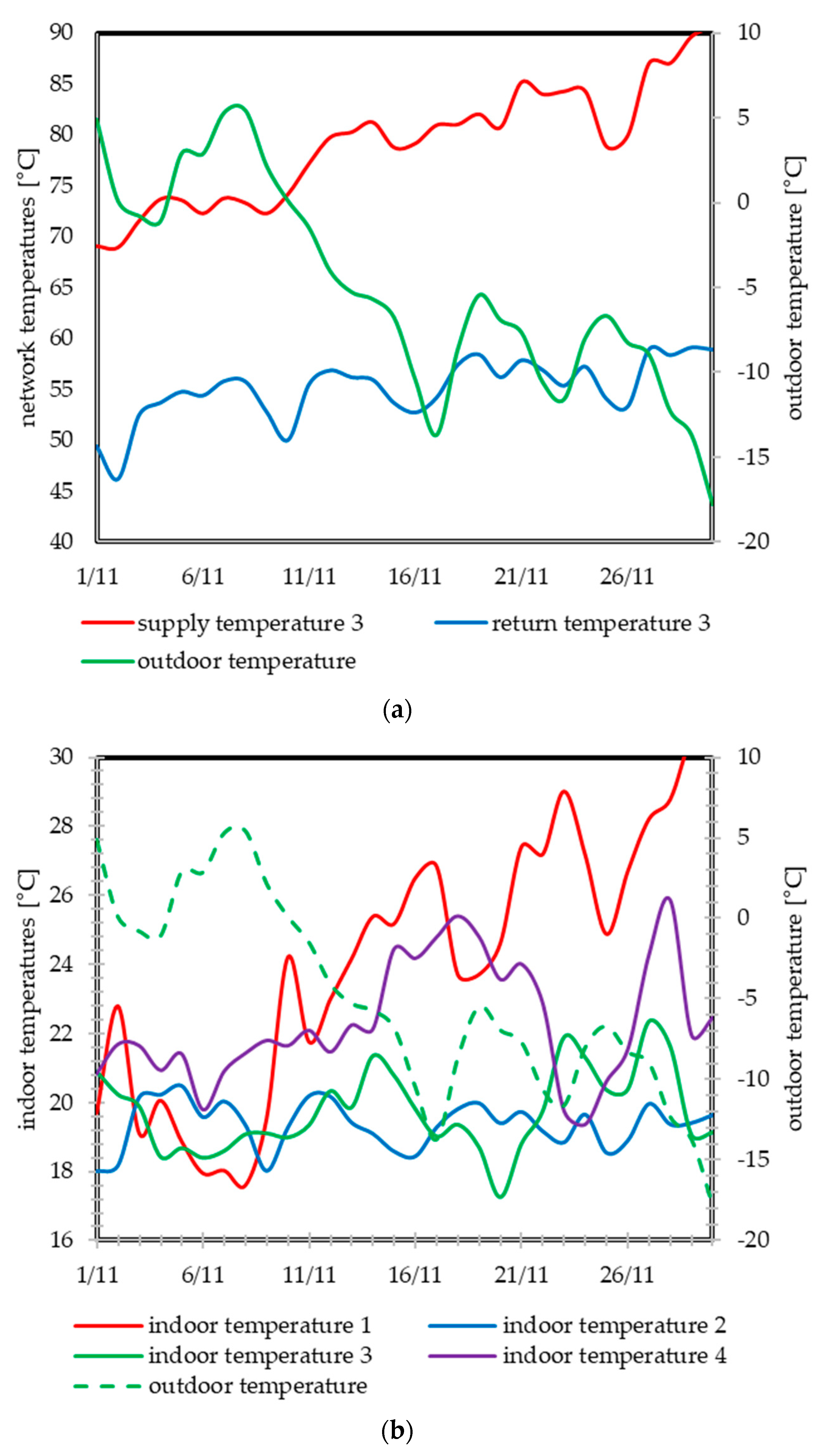
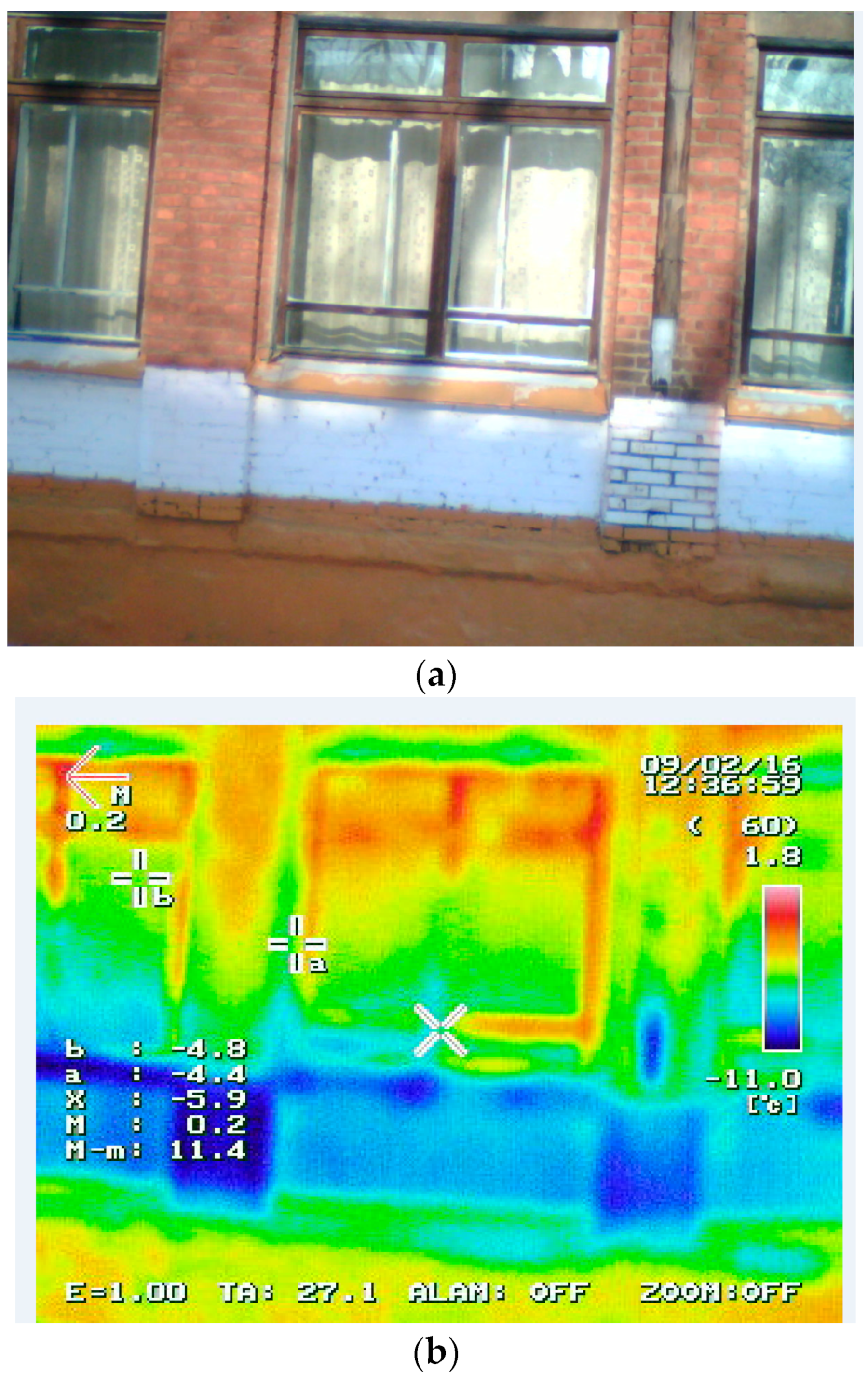
4. Results and Discussion

Using operational data is the easiest way to comprehend a delay direction between indoor temperature and comprehensive outdoor temperature. The positive and negative of delay time l represents the delay between indoor and outdoor temperature. A correlation factor of 0.54 determines mediocre but positive interconnection between the variables. In addition, because of the dynamic variations in flow rate and supply temperature, the time lag and moving window size may differ depending on the building structure (Figure 4).

Figure 4 details the large differences in temperature levels, which occur among the sets of studied buildings. Newer buildings have generally lower but smoother profiles of indoor temperature (the third indoor temperature curve), while the older panel-built buildings (the second one) are much less energy-efficient. There is also a building (the first indoor temperature curve) characterized by a more fluctuating and stochastic heating pattern, which indicates malfunctioning of a valve.

For 89% of studied buildings, it was obvious that the indoor temperature profile clearly followed outdoor temperature; their profiles were close to the second and the third indoor temperature curves; therefore, they are not shown separately. For the rest of the buildings, the indoor temperature was unreasonably high, being about 25–30 °C. There were three buildings where the indoor temperature did not closely correlate with the outdoor temperature; better understanding of external factors affecting indoor temperature here could be a potential option as well. For instance, for the first and the fourth indoor temperature curves, it was noticeable that the control strategy of the secondary SH supply temperature setpoint might require adjustment to keep both the indoor temperature and return temperature lower. However, the faulty valve was not a reason here; thus, the primary reason was relevant to investigate. The results of the visual study are reported below.

To compare numeric values, Ivanko et al. [5] studied heat consumption during the warm months, and introduced control point temperature, CPT, which is the outdoor temperature above which a certain amount of heat is consumed by SH: 16 °C. Jangsten et al. [28] studied district cooling systems and focused on return temperature; they gave the highest threshold of 16 °C, which is 100% more than the normal values. As observable from Ivanko et al.’s research [5], another reason for the discrepancy is higher than design heat demand. They also hypothesized about overconsumption of the heat exchanger control valve connecting the SH system to the DH network, which had wrongly dimensioned or malfunctioned. This led to the SH heat use in spring, summer, and fall, when the control valve was expected to be fully shut.

In Russia, control valves typically pass an excessive amount of the water flow when compared with designs (Figure 4). This effect begins when the outdoor temperature decreases and the heating season starts; therefore, it only happens in late fall, winter, and early spring. The reason is that the supply temperature or flow rate have to increase to compensate for additional heat losses. That means that in Omsk and Krasnoyarsk, supply temperature correlates not only with the outdoor temperature, but also depends on the performance of envelopes. This may clarify why the actual indoor temperature does not follow the design profile shown in Figure 4.

Figure 5 illustrates the impact of the different types of additional thermal mass on the building’s indoor temperature compared with the empty room reference cases.

In such buildings, heat demands increase sharply around 8 a.m. (when the working day begins) and then run high until approx. 5 p.m., in both old and new buildings. However, in the case of the latter, it decreases gradually at midday and only accounts for 15–20% at 12–2 p.m., when heat insolation and internal heat gains are the highest. As a result, it has a circadian cycle.

However, the indoor temperature in the real building was higher than the modeling prediction by up to 2 °C on average. This may be associated with insolation and the fact that buildings retain the energy accumulated during the periods when the indoor target temperature is 20 °C. This is still much lower compared with the discrepancy of 10 °C between actual values (up to 30 °C) and design (fixed 20 °C). Unlike that, in Luc et al.’s paper [8], the discrepancy between real-world scenarios and simulations was greater during the night-time, as heat generation costs are typically lower during night-time. As such, more of the periods with increased setpoint happened during night-time. However, the methodology without time-dependent variables is not capable of adapting without relying on dynamic deployment.

The developed correlation with envelope conditions is presented in Figure 6.

Despite the potential use of heat accumulation capacity of building envelopes, the compensation times to reduce heat delivery from a DH plant are not sufficient. This means that under usual operating conditions and typical outdoor temperatures, this factor is negligible.

Figure 6 clearly indicates that an additional amount of energy is required every second to cover all these leakages. It is essential to compare temperature fields during normal operating conditions to the amount of energy required to increase the temperature when a much more intensive process of infiltrating outdoor air occurs. This enables quantification of the additional amount of energy required to account for poor insulation (minus internal heat gains) and the energy required to ensure indoor comfort.

In Camci et al.’s [25] study, the same heat transfer coefficient correlations were developed to be used in the heat demand calculations of a particular office room. However, the first difference was an emphasis on convective heat transfer; the second difference was the studied room being equipped with a thermal-activated cooled wall; and the third difference was that the experiments were performed using a TRNSYS simulation model and a thermal test compartment. Convective heat transfer coefficient values versus distance from the diffuser were plotted with two air speed values and two temperature difference values, which are also quite different and hard to compare.

The insights reveal that it is relevant to calculate compensation times ranging from 16.1 h to 0.6 h (as much as 284.4 h to 1.9 h in [29]) using the internal energy capacity of buildings, with the lowest reduction in the indoor temperature of 1 K and the highest of 6 K achieved, respectively (1 and 6 °C in [29], respectively). Utilizing the heat-accumulating ability of the building’s envelopes, these compensation times can be determined to balance the heat supply of the DH plant.

The model for envelopes has been expanded with occupancy profiles and validated by visual inspections, based on survey data (Figure 5 and Figure 6). For comparison, Harney et al. [21] established and validated occupancy profiles solely with the help of survey data provided by the Technological University of the Shannon (Ireland).

The initial and the corrected heat demands of the reference building are listed in

Table 2. Distribution of design and actual heat demand.

#	Office (Zone)	Design Heat Demand [W]	Due to Infiltration [W]	Heat Gains [W]	Actual Heat Demand [W]
Column	1	2	3	4	5
Remark		Refer to Equation (2)	Refer to Equation (4)	Refer to [26]	Column #2 + Column #3 − Column #4
Ground floor
1	Tool shop	6325	12,689	n/a	19,014
2	Storage room for household chemical goods, garage	7899	17,168	n/a	25,067
					∑44,081
First floor
13	Office	708	1124	411	1421
4	Exhibition hall	17,294	24,132	9028	32,398
2	Vestibule	936	1300	n/a	2236
3	Office	4720	965	467	5218
12	Exhibition hall	8569	19,191	7014	20,746
	Staircase	1102	560	n/a	1662
	Staircase	1334	590	n/a	1924
					∑65,605
Second floor
12	Office	16,822	11,664	2209	26,277
6	Hallway	2001	5395	n/a	7396
11	Office	2375	1322	485	3212
19	Office	1164	858	538	1484
1	Office	657	2356	358	2655
2	Office	1731	3275	1223	3783
3	Office	1731	3275	1223	3783
4	Office	2224	6781	2291	6714
5	Office	2494	1634	765	3363
10	Office	8155	5258	1836	11,577
14	Office	6476	5365	3498	8343
20	Office	3976	2630	1649	4957
					∑83,544
Third floor
14	Office	12,754	8973	2328	19,399
5	Office	6341	3110	1703	7748
1	Security room	961	1440	n/a	2058
13	Hallway	1376	2997	n/a	4373
9	Lounge	4975	2039	745	6269
6	Exhibition hall	6990	4805	n/a	11,795
7	Vestibule	422	108	n/a	530
3	Vestibule	386	85	n/a	471
15	Vestibule	351	108	n/a	459
					∑53,101
Fourth floor
1	Reception	4565	2730	998	6297
2	Principal’s office	4569	2924	1069	6424
3	Lounge area	2509	1026	396	3139
4	Bathroom	502	233	n/a	735
					∑16,595
Total					262,926

.

Table 2 highlights the differences between traditionally obtained values and actual heat demand. The actual energy demand may be defined using the actual rate of heat losses for a given building construction and design consumption profile. Once the indoor temperature is constant, the actual rate of heat losses is defined as the point where the heat generated accounts for the sum of heat consumed and lost. The lack of heat demand in Table 2 in the middle of the building (mainly hallways) is caused by the limited surface area contacting outer walls and the temperature not dropping below the target value (taking into account the allowed control error). The energy-saving effect might be achieved by allowing all the surplus energy to be dumped into the building envelopes and all the deficit to be supplied by the peak units. This means the flow rate or supply temperature is varied in the narrower range to ensure indoor comfort for the given conditions.

5. Conclusions

There are eight main factors affecting indoor temperature in the case of district heating: primary (network) supply temperature; secondary (space heating) supply temperature; return temperature; state of the space heating system (incl. radiators); envelope state (incl. infiltration); thermal inertia; internal heat gains; and solar insolation (incl. glazing share and building orientation).

To consider five factors, correction factors have been suggested. The methodology enables detection of the indoor spaces with additional heat losses and gains. To assess more precise SH consumption profiles, the results are best input into BIM software [30,31]. The suggested methodology may also lead to lower peaks of heat demand compared with the traditional methodology. This is especially helpful to reduce daily peaks. The storage cycle may start from the surplus time step (5:00). Then, the energy delivery from a DH plant can be reduced until the capacity of envelopes tends negative at any certain time step. The building envelopes ease charging to the maximum storage capacity to balance given generation and demand profiles, which are the key factors when guiding the investments to achieve meaningful reductions in GHG emission.

In addition, once heat demand is covered according to the maximum storage capacity for the given generation and demand profiles, fewer efforts to modernize a DH are required. Through the obtained results, useful design criteria, new indicators, and more data can be provided to designers, energy and construction engineers, industry decision-makers, and key stakeholders, such as local authorities.

References

1. Buffa, S.; Cozzini, M.; D’Antoni, M.; Baratieri, M.; Fedrizzi, R. 5th generation district heating and cooling systems: A review of existing cases in Europe. Renew. Sustain. Energy Rev. 2019, 104, 504–522. [Google Scholar] [CrossRef]
2. Wirtz, M.; Kivilip, L.; Remmen, P.; Müller, D. 5th Generation District Heating: A novel design approach based on mathematical optimization. Appl. Energy 2020, 260, 114158. [Google Scholar] [CrossRef]
3. Vandermeulen, A.; van Oevelen, T.; van der Heijde, B.; Helsen, L. A simulation-based evaluation of substation models for network flexibility characterisation in district heating networks. Energy 2020, 201, 117650. [Google Scholar] [CrossRef]
4. Guelpa, E. Impact of thermal masses on the peak load in district heating systems. Energy 2021, 214, 118849. [Google Scholar] [CrossRef]
5. Ivanko, D.; Sørensen, Å.L.; Nord, N. Splitting measurements of the total heat demand in a hotel into domestic hot water and space heating heat use. Energy 2021, 219, 119685. [Google Scholar] [CrossRef]
6. Braas, H.; Jordan, U.; Best, I.; Orozaliev, J.; Vajen, K. District heating load profiles for domestic hot water preparation with realistic simultaneity using DHWcalc and TRNSYS. Energy 2020, 117552. [Google Scholar] [CrossRef]
7. Chicherin, S.; Starikov, A.; Zhuikov, A. Justifying network reconstruction when switching to low temperature district heating. Energy 2022, 248, 123618. [Google Scholar] [CrossRef]
8. Luc, K.M.; Li, R.; Xu, L.; Nielsen, T.R.; Hensen, J.L.M. Energy flexibility potential of a small district connected to a district heating system. Energy Build. 2020, 225, 110074. [Google Scholar] [CrossRef]
9. Johra, H.; Heiselberg, P.; Le Dréau, J. Influence of envelope, structural thermal mass and indoor content on the building heating energy flexibility. Energy Build. 2019, 183, 325–339. [Google Scholar] [CrossRef]
10. Chicherin, S. A method for assessing heat losses in developing countries with a focus on operational data of a district heating (DH) system. Sustain. Energy Grids Netw. 2022, 30, 100616. [Google Scholar] [CrossRef]
11. Chicherin, S.; Zhuikov, A.; Kolosov, M.; Junussova, L.; Aliyarova, M.; Yelemanova, A. Optimizing building heat consumption: Weekday and weekend profiles. Energy Rep. 2021, 7, 166–170. [Google Scholar] [CrossRef]
12. Jebamalai, J.M.; Marlein, K.; Laverge, J. Influence of centralized and distributed thermal energy storage on district heating network design. Energy 2020, 202, 117689. [Google Scholar] [CrossRef]
13. Sleptsov, A.; Crisostomi, E.; Bischi, A. Control schemes for district heating substations considering user-defined building’s indoor temperature. Build Environ. 2021, 191, 107598. [Google Scholar] [CrossRef]
14. Sommer, T.; Sulzer, M.; Wetter, M.; Sotnikov, A.; Mennel, S.; Stettler, C. The reservoir network: A new network topology for district heating and cooling. Energy 2020, 199, 117418. [Google Scholar] [CrossRef]
15. Patureau, R.; Tran, C.T.; Gavan, V.; Stabat, P. The new generation of District heating & cooling networks and their potential development in France. Energy 2021, 236, 121477. [Google Scholar]
16. Romanov, D.; Pelda, J.; Holler, S. Technical, economic and ecological effects of lowering temperatures in the Moscow district heating system. Energy 2020, 211, 118680. [Google Scholar] [CrossRef]
17. Saletti, C.; Zimmerman, N.; Morini, M.; Kyprianidis, K.; Gambarotta, A. Enabling smart control by optimally managing the State of Charge of district heating networks. Appl. Energy 2020, 283, 116286. [Google Scholar] [CrossRef]
18. Farouq, S.; Byttner, S.; Bouguelia, M.-R.; Nord, N.; Gadd, H. Large-scale monitoring of operationally diverse district heating substations: A reference-group based approach. Eng. Appl. Artif. Intell. 2020, 90, 103492. [Google Scholar] [CrossRef]
19. Gadd, H.; Werner, S. Achieving low return temperatures from district heating substations. Appl. Energy 2014, 136, 59–67. [Google Scholar] [CrossRef]
20. Ren, C.; Cao, S.J. Construction of linear temperature model using non-dimensional heat exchange ratio: Towards fast prediction of indoor temperature and heating, ventilation and air conditioning systems control. Energy Build. 2021, 251, 111351. [Google Scholar] [CrossRef]
21. Harney, P.; Gartland, D.; Murphy, F. Determining the optimum low-temperature district heating network design for a secondary network supplying a low-energy-use apartment block in Ireland. Energy 2020, 192, 116595. [Google Scholar] [CrossRef]
22. Fitó, J.; Hodencq, S.; Ramousse, J.; Wurtz, F.; Stutz, B.; Debray, F.; Vincent, B. Energy- and exergy-based optimal designs of a low-temperature industrial waste heat recovery system in district heating. Energy Convers. Manag. 2020, 211, 112753. [Google Scholar] [CrossRef]
23. Quirosa, G.; Torres, M.; Soltero, V.M.; Chacartegui, R. Energetic and economic analysis of decoupled strategy for heating and cooling production with CO2 booster heat pumps for ultra-low temperature district network. J. Build. Eng. 2022, 45, 103538. [Google Scholar] [CrossRef]
24. Sun, C.; Chen, J.; Cao, S.; Gao, X.; Xia, G.; Qi, C.; Wu, X. A dynamic control strategy of district heating substations based on online prediction and indoor temperature feedback. Energy 2021, 235, 121228. [Google Scholar] [CrossRef]
25. Camci, M.; Karakoyun, Y.; Acikgoz, O.; Dalkilic, A.S. A comparative study on convective heat transfer in indoor applications. Energy Build. 2021, 242, 110985. [Google Scholar] [CrossRef]
26. SP 50.13330.2012; Thermal Protection of Buildings. RussianGost|Official Regulatory Library: Moscow, Russia, 2018.
27. Federal Law. ‘On Energy Saving and on Increasing Energy Efficiency and on Amendments to Certain Legislative Acts of the Russian Federation’ of 23.11.2009 N 261-FZ; Food and Agriculture Organization of the United Nations: Rome, Italy, 2009. [Google Scholar]
28. Jangsten, M.; Lindholm, T.; Dalenbäck, J.O. Analysis of operational data from a district cooling system and its connected buildings. Energy 2020, 203, 117844. [Google Scholar] [CrossRef]
29. Turski, M.; Sekret, R. Buildings and a district heating network as thermal energy storages in the district heating system. Energy Build. 2018, 179, 49–56. [Google Scholar] [CrossRef]
30. He, R.; Li, M.; Gan, V.J.L.; Ma, J. BIM-enabled computerized design and digital fabrication of industrialized buildings: A case study. J. Clean. Prod. 2021, 278, 123505. [Google Scholar] [CrossRef]
31. Jang, R.; Collinge, W. Improving BIM asset and facilities management processes: A Mechanical and Electrical (M&E) contractor perspective. J. Build. Eng. 2020, 32, 101540. [Google Scholar]
Figure 1. Correction to the diurnal thermal load variation in individual spaces according to the orientation.
Sustainability 15 15603 g001
Figure 2. The layout of a DH substation: isolating valve 1; valves 2, 12; filters 3, 5; gauge position/back-up air-release valve 6; back-up pressure sensors 7, 8; air-release valve 9; circulation pump 10; check valve 11; drainage valve 13; back-up drainage valve 14; back-up temperature sensor 15; pressure sensors 16; regulating valve 17; straight pipe 18; automatic controller 20; temperature sensor (for a controller) 21; heat meter 22; flow meter 22.1; and temperature sensor (for a heat meter) 22.1.
Sustainability 15 15603 g002
Figure 3. New office building located in Omsk, Russia. All the details of the indoor spaces simulated in this research are based on its blueprints.
Sustainability 15 15603 g003
Figure 4. The relationship between secondary supply/return temperatures (a) and indoor and outdoor temperatures (b). Profiles #1 and #2 refer to the archetypes of older panel-built buildings (before 1990); #3 and #4 refer to newer ones.
Sustainability 15 15603 g004
Figure 5. Comparison of the visual representation (at the top, a) and thermography (at the bottom, b) for heat leaking.
Sustainability 15 15603 g005
Figure 6. Distribution of temperature and mixing energy flows next to the window zone: visible range (a) and thermography (b) images.
Sustainability 15 15603 g006