Optimal Protection Scheme for Enhancing AC Microgrids Stability against Cascading Outages by Utilizing Events Scale Reduction Technique and Fuzzy Zero-Violation Clustering Algorithm

Abstract

The precision with which directional overcurrent relays (DOCRs) are set up establishes the microgrid customers’ access to reliable and uninterrupted electricity. In order to avoid failure in DOCRs operation, it is critical to consider a single contingency (N-1 event) on the protection optimization setting problem (POSP). However, power systems may face cascading outages or simultaneous contingencies (N-K events), which greatly expand the problem’s complexity and scale. The effect of cascading events on this problem is an open research gap. Initially, this paper proposes a novel approach to reducing the scale of simultaneous events called the N-K events scale reduction technique (N-K-ESRT). Moreover, an innovative method named fuzzy zero-violation clustering is utilized to group these contingencies. Ultimately, the DOCRs’ decision parameters are generated by three optimization algorithms, namely interior point (IPA), simulated annealing, and pattern search. In all case studies (including a real industrial network called TESKO2 feeder, the IEEE Std. 399-1997, and the IEEE 14 bus systems), the capabilities of the proposed method are effectively validated based on the DOCR’s tripping time and the algorithm’s execution time.

1. Introduction

Generation, transmission, sub-transmission, and distribution networks are the four arms that constitute the whole electrical grid. The most critical and vital protective devices in distribution networks are overcurrent relays (OCRs) and DOCRs, which operate in the event of a fault. The fundamental task of protective relays is to quickly identify a permanent fault and transmit the tripping signal to the circuit breaker. The accurate setting of primary relays (main relays) is at the core of the fundamental architecture governing protective coordination, which is subsequently backed up by secondary relays (backup relays) at regular intervals. In traditional distribution networks, OCRs are the primary protection devices due to the radial orientation of the network’s current [1,2]. The conventional electrical distribution network has recently been transformed into a microgrid as a consequence of the penetration of distributed generation (DG) units [3,4]. This resulted in the conception of microgrids, in which DGs can feed the distribution network with or without a power grid link [5,6]. Due to the multiple orientations of electric current in microgrids, protection schemes are based on DOCRs [7,8]. The DOCR setting parameters (DSPs) contain the current setting parameter (CSP) and the time setting multiplier parameter (TSMP).

The TSMP regulates the time required for the relay to trip, and the CSP is equal to the current flowing through the secondary side of the relay’s current transformer (CT) [9,10]. The time-current characteristic of DOCRs is specified by both the current and time-setting parameters. Due to the nonlinearity of the POSP of DOCRs, nonlinear programming (NLP) is advised to answer the POSP [11,12]. In acknowledgment of the lack of advancement in heuristic and meta-heuristic optimization algorithms (MOAs) during the last decades, linear approaches (i.e., the simplex, two-phase simplex, and dual simplex programming) have been employed to assess the DOCR setting parameters [13]. In this literature, the POSP was formed using linear programming (LP) with the notion that one of the DSPs is given. In recent years, MOAs have been widely deployed to swiftly handle NLP without damaging the convexity of POSP. The noteworthy MOAs that have been employed to figure out the best outcomes of POSP include improved firefly optimization algorithm (IFOA) [9], improved moth-flame optimization algorithm (IMFOA) [10], imperialistic competition optimization algorithm (ICOA) [11], improved seagull optimization algorithm (ISOA) [12], chaotic search class topper optimization algorithm (CSCTOA) [13], the genetic algorithm (GA) [6,8,14,15,16,17], grey wolf optimization algorithm (GWOA) [17], and partial swam optimization (PSO) [15,18].

The disadvantages of MOAs, such as their penchant for early convergence at local points and the excess time needed to solve the POSP, can be alleviated by applying hybrid algorithms [19,20]. The outcomes achieved by hybrid algorithms in the referenced literature reveal the superiority of these techniques over others in tackling the malfunction of the DOCRs. In hybrid algorithms, the POSP is partitioned into sub-problems, each of which is addressed using a distinct strategy. In recent studies, hybrid algorithms, such as the hybrid whale optimization algorithm (HWOA) [19], GA-LP [20,21], PSO-LP [20], hybrid simulated annealing optimization algorithm (SAOA) and LP (HSAOA-LP) [22], hybrid ant colony optimization algorithm (HACOA) [23], hybrid gradient-based optimizer (HGBO) [24,25], hybrid opposition-based learning fractional order class topper optimization algorithm (HOBL-FOCTOA) [26], IPA [27], firefly algorithm (FA) and target remedy [28], fuzzy logic and GA [29], GA-PSO with differential evolution (DE) algorithm (GA-PSO-DE) [30], and FA-LP [31] have been devised. In addition, machine learning approaches facilitate the computation of DSPs. Furthermore, ref. [4] designed a protection scheme based on deep reinforcement learning (DRL) and long short-term memory (LSTM)-enhanced deep neural networks. Also, refs. [5,6,7,8] provided the clustering algorithms to group diverse network topologies into a small subset with k-means, pre-computed offline setup groups with storing memory, and self-organizing maps (SOM). To remedy the problem of low fault current contributions of inverter-based DGs (IBDGs), ref. [1] intends harmonic DOCR (HDOCR) with leveraging the current injection capability of IBDGs; ref. [2] exemplifies a third harmonic voltage produced by the IBDGs controller throughout fault currents; and ref. [3] refers to virtual impedance-fault current limiters (IFCLs).

The conventional methods of POSP were founded on the immutability of the grid topology (fixed topology (FT)). Nonetheless, electrical equipment failures (i.e., outages of lines, loads, DGs, synchronous machines, etc.) may alter the structure of the distribution grid [3]. This issue causes the CSP and fault currents of the network to fluctuate, ultimately resulting in incorrect relay operation [5,6]. To prevent the violation (i.e., miscoordination) of DOCRs, the literature advocated incorporating contingencies such as line outages [32], DG outages [33,34], a single contingency for all presumed equipment [3], and an islanding mode [1,2,3] into the POSP.

Hence, a comprehensive literature review is provided in

Table 1. Summary of the literature review in the field of POSP of DOCR.

Reference	Year	Dual-Setting	Double Inverse	MSGs	HDOCR	SCD	N-SCD	SSSCD	FT	N-1 Contingency	N-2 Contingencies	Islanded Mode	PCAC	MOOP	Optimization Algorithm
[1]	2020	✘	✘	✘	✔	✘	✘	✘	✔	✘	✘	✔	✘	✘	-
[2]	2020	✘	✘	✘	✔	✘	✘	✘	✔	✘	✘	✔	✘	✘	-
[3]	2021	✘	✘	✘	✔	✘	✘	✘	✔	✔	✘	✔	✔	✘	-
[5]	2022	✘	✘	✔	✘	✔	✘	✘	✔	✔	✘	✔	✘	✘	-
[6]	2018	✘	✘	✔	✘	✔	✘	✘	✔	✔	✘	✘	✘	✘	GA
[7]	2021	✘	✘	✔	✘	✔	✘	✘	✔	✔	✘	✘	✘	✔	-
[9]	2019	✘	✘	✘	✘	✔	✘	✘	✔	✘	✘	✘	✘	✘	IFOA
[10]	2020	✘	✘	✘	✘	✔	✔	✔	✔	✘	✘	✘	✘	✘	IMFOA
[11]	2021	✘	✘	✘	✘	✔	✘	✘	✔	✘	✘	✘	✘	✘	ICOA
[12]	2022	✘	✘	✘	✘	✔	✘	✘	✔	✘	✘	✘	✘	✘	ISOA
[13]	2022	✘	✘	✘	✘	✔	✘	✘	✔	✘	✘	✘	✘	✘	CSCTOA
[14]	2018	✘	✘	✘	✘	✔	✘	✔	✔	✘	✘	✘	✘	✘	GA
[16]	2023	✔	✘	✘	✘	✔	✘	✔	✔	✘	✘	✔	✘	✘	GA
[17]	2022	✔	✘	✘	✘	✔	✘	✔	✔	✘	✘	✘	✘	✘	GA/GWOA
[18]	2023	✘	✘	✘	✘	✘	✔	✘	✔	✘	✘	✘	✘	✘	PSO
[19]	2019	✘	✘	✘	✘	✔	✘	✘	✔	✘	✘	✘	✘	✘	HWOA
[20]	2021	✘	✘	✘	✘	✔	✘	✘	✔	✔	✘	✔	✘	✘	GA-LP/PSO-LP
[21]	2019	✘	✘	✘	✘	✔	✘	✘	✔	✔	✘	✘	✘	✔	GA-LP
[22]	2020	✘	✘	✘	✘	✔	✘	✘	✔	✘	✘	✘	✘	✘	HSAOA-LP
[23]	2019	✘	✘	✘	✘	✔	✘	✘	✔	✘	✘	✘	✘	✘	HACOA
[24]	2021	✘	✘	✘	✘	✔	✘	✘	✔	✘	✘	✘	✘	✘	HGBO
[25]	2022	✘	✘	✘	✘	✔	✘	✔	✔	✘	✘	✘	✘	✘	HGBO
[26]	2021	✘	✘	✘	✘	✔	✘	✘	✔	✘	✘	✘	✘	✘	HOBL-FOCTOA
[27]	2019	✘	✘	✘	✘	✔	✘	✘	✔	✘	✘	✘	✘	✔	IPA
[28]	2021	✘	✘	✘	✘	✔	✔	✘	✔	✘	✘	✘	✘	✘	FA-Target Remedy
[29]	2023	✘	✘	✘	✘	✔	✔	✘	✔	✘	✘	✘	✘	✘	GA-Fuzzy Logic
[30]	2020	✘	✘	✘	✘	✔	✔	✔	✔	✘	✘	✘	✘	✘	GA-PSO-DE
[31]	2022	✘	✘	✘	✘	✔	✔	✘	✔	✘	✘	✘	✘	✘	FA-LP
[32]	2022	✘	✘	✘	✘	✔	✘	✘	✔	✔	✘	✔	✘	✘	HGA-LP

- stands for no data.

to establish the existing knowledge and gaps for microgrid protection in terms of published year, dual-setting DOCR, double inverse characteristic of DOCR, and multiple setting groups (MSGs).

DOCR, HDOCR, standard characteristic of DOCR (SCD), non-standard characteristic of DOCR (N-SCD), smart selection of SCD (SSSCD), FT, N-1 contingency, N-2 contingencies, island mode, POSP of DOCR based on communication assisted scheme (PCAC), multi-objective optimization of problem (MOOP), and optimization algorithm.

In this table, the literature review has been summarized. As seen, there is a research gap in the literature because N-2 contingencies have not been studied in the available references in the POSP of DOCR.

In previous decades, a blackout occurred in Europe on 4 November 2006, and in India on 30–31 July 2012, as a result of cascading events [35,36]. The following report excerpt is also included in [37], which contains the annual report for Nordic and Baltic system disruption statistics in 2020.

“Bus 1 (420 kV) in Halden was out of service due to a circuit breaker failure in Sweden. Simultaneously, Bus 2 (420 kV) in Halden is out of service for maintenance. Due to these events, 310 MWh of energy were not supplied, including the interruption of 240 MW of industrial load such as the production of paper”.

Consequently, according to the cited literature and a recent report of power grid disturbances, simultaneous events result in a significant grid disconnection. The possibility of these occurrences is imminent and will result in substantial economic and reliability losses for sensitive loads.

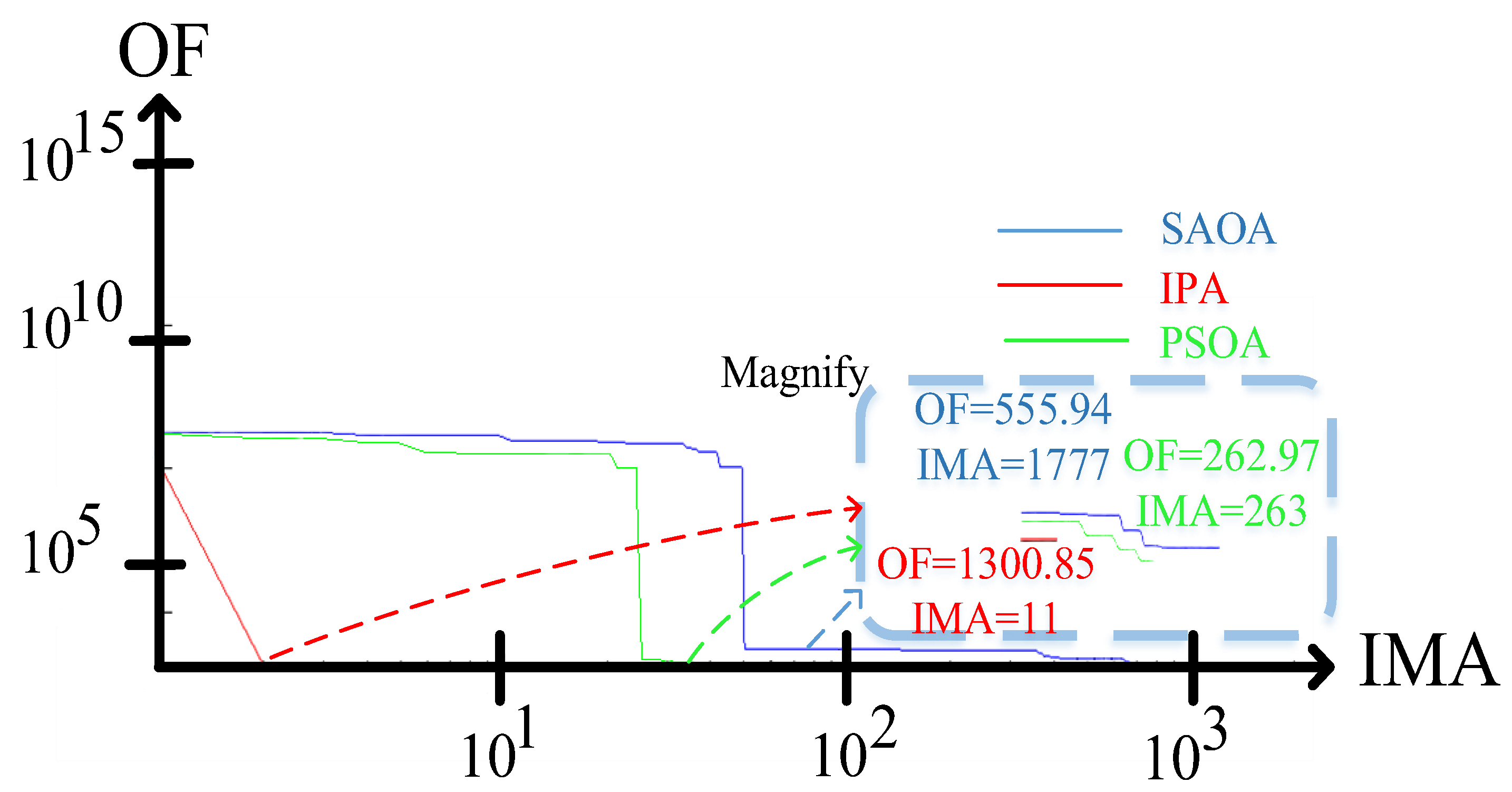
In this paper, the DOCR setting parameters are determined by evaluating N-2 contingencies in order to safeguard the network against a blackout. Cascading failures dramatically increase the problem model’s complexity and size. In order to reduce the dimensions of the POSP, an innovative technique named N-K-ESRT is offered. As a result of this technique’s foundation, all contingency scenarios are reduced to a much smaller subset, and the POSP only analyzes these chosen contingencies. Subsequently, an innovative clustering technique, namely the fuzzy zero-violation clustering algorithm (F-ZVCA), is applied to group the chosen contingencies in order to avoid the miscoordination of DOCRs. The IPA, SAOA, and pattern search optimization algorithm (PSOA) are ultimately employed to pinpoint the DSPs for each cluster. The most noteworthy contributions of this paper might be summarized as follows:

• An innovative scale reduction technique called N-K-ESRT is utilized to decrease the scale of the N-2 contingencies.
• The F-ZVCA is proposed to eradicate the DOCR’s miscoordination and reduce the scope of the POSP.
• The distinguish MOAs are recommended for determining the best DSPs.
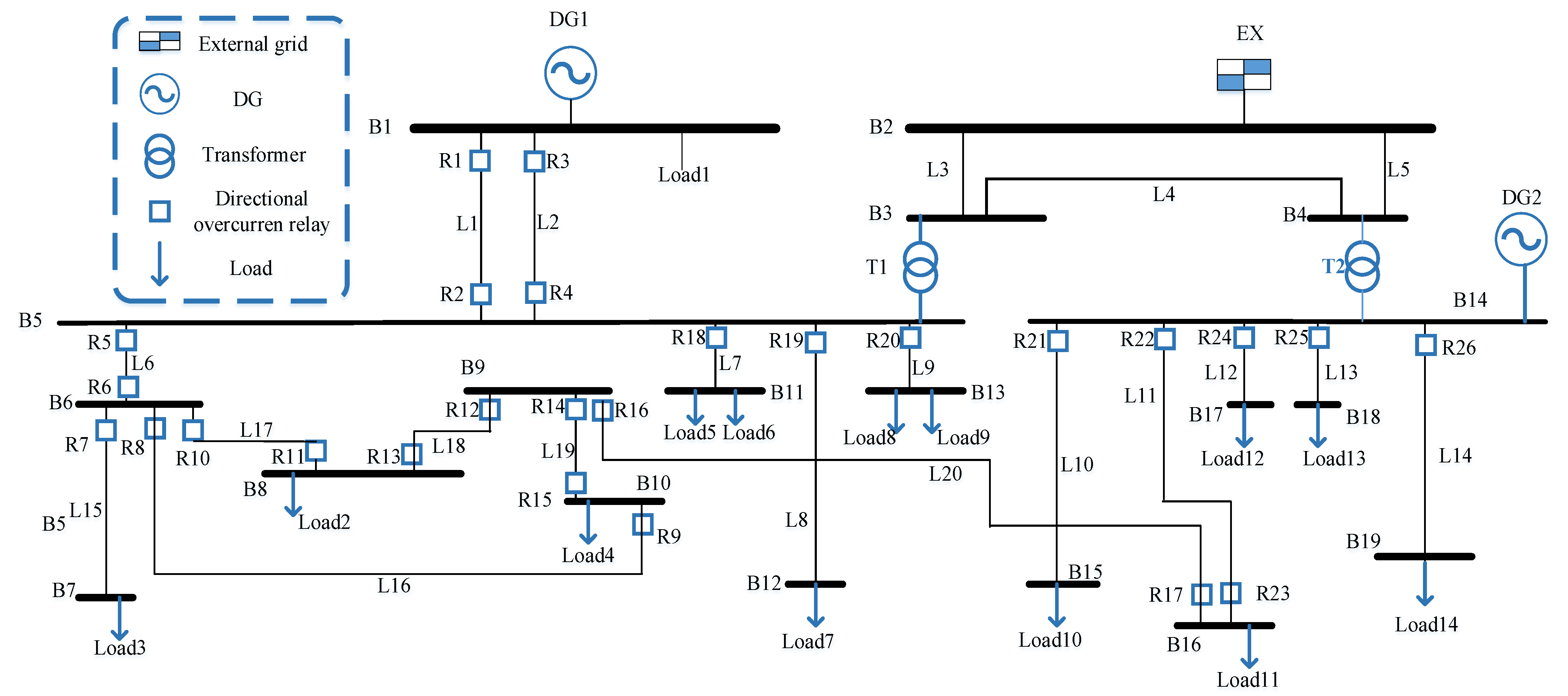
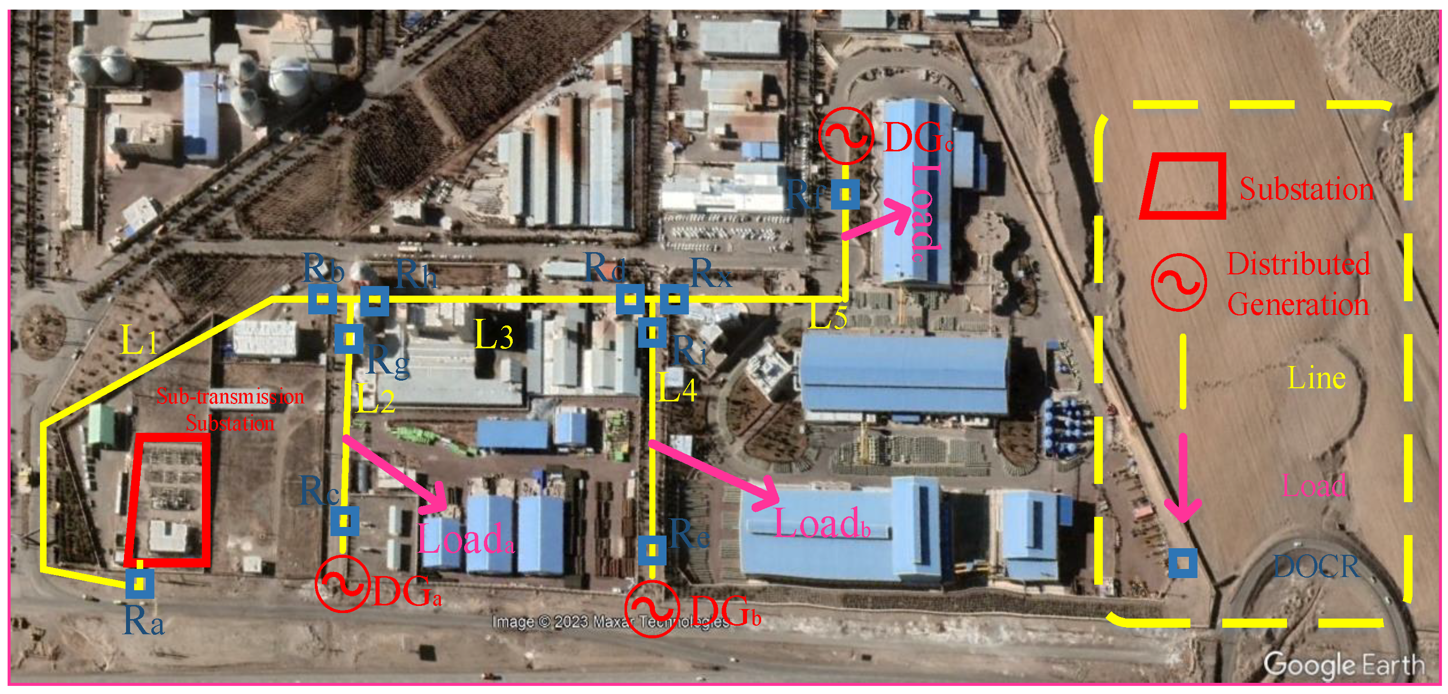
• The offered solving procedure is applied to three AC microgrids, including a real distribution system (named TESKO2 feeder), besides the IEEE Std. 399-1997 and IEEE 14 bus systems.

2. Problem Modeling of DOCRs

The major purpose of the objective function (OF) is to decrease the operating time of the installed DOCRs while preventing miscoordination. Despite this, when cascading failures are factored into the POSP, the likelihood of DOCR’s miscoordination skyrockets compared to a single outage. Consequently, during the optimization procedure, one of the major challenges is to completely eradicate the miscoordination of DOCRs. The OF of the problem model (1) and the associated relations and constraints, including the operation time of DOCRs (2), the miscoordination relation (3), the miscoordination constraint (4), the TMSP constraint (5), and the CSP constraints (6)–(7), are stated below. Also, it should be highlighted that all aforementioned relations (i.e., (2)–(7)) must be established for all network structures (i.e., index S), all main relays (i.e., index M), and their backup relays (i.e., index JB).

2.1. Objective Function

The objective function of the problem consists of two parts in (1). The prime focus of the first part is to optimize the operation time of all DOCRs. In fact, part 1 is the total operating time of all DOCRs that are installed in the related case study. On the other hand, the key aim of part 2 is to eliminate DOCR miscoordination between the primary DOCR and its backup relays. In actuality, invalid DSPs significantly increase the value of the OF (due to the penalty factor), and the problem model initially aims to eliminate this barrier by minimizing part 2. $\mathsf{\eta }$ is used as the penalty factor of the OF to prohibit miscoordination (or invalid DSP) that results in a negative $\mathsf{\delta }T.$ Following this, the problem model designates the DSPs that are attempting to optimize the initial part among those that have contributed to the precise coordination of part 2. The OF can be represented by the following equation:

$$\left\{OF=\stackrel{}{Optimization}(\frac{〈{\displaystyle \sum _{M=1}^Q(T^{M,S})}〉}{part 1}+\frac{〈\mathsf{\eta }\times \mathrm{\delta }{T}_{}^{MJB,S}〉}{part 2})\right\}$$

(1)

2.2. DOCRs Relations and Constraints

Equation (2) is the operating time (tripping time) of DOCR based on the inverse time characteristic of the IEC 60255-3 standard [5]. The operating time of the relay is dependent on the DSPs and the fault current passing through the Mth relay (I_FC). The values of DSPs are directly proportional to the DOCR’s operational time. In contrast, assuming the DSPs are fixed, (2) demonstrates that the operation time of DOCRs is inversely proportional to the fault current magnitude. Fault current is considered the near-end three-phase to ground faults.

As was previously established, the cornerstone of the POSP is the accurate setting of DOCRs without miscoordination and the minimization of the OF. Miscoordination occurs when a backup relay works before its primary relay. Due to the possibility of system lags such as a time delay in DOCR’s CT, the miscoordination relation (3) considers 0.2 s as the time gap between the operation time of the primary relay and its backup DOCRs, which is called the coordination time interval (CTI). Moreover, η is employed as the penalty factor of the POSP to prohibit the miscoordination that leads to violation of the miscoordination constraint (i.e., negative $\mathsf{\delta }T$), which is stated as (4).

In addition, (5) and (6) provide the upper and lower bounds for CSP and TSMP, respectively. The TSMP is modified in increments of 0.01 s between 0.05 s and 1 s. Furthermore, the CSP limit is between 0.1 A and 4 A, in increments of 0.1, assuming the current on the secondary side of the CT is 1 A. The boundary limits for TSMP and CSP are specified by the relay manufacturers. Here, the presumed DOCR is the SIPROTEC (i.e., Siemens protection relays) 7SJ64 multifunction numerical overcurrent relay, a Siemens manufacturing product [38]. Also, POSP in this paper is expressed as mixed integer nonlinear programming (MINLP) since CSP and TSMP are characterized discretely and continuously, respectively. Consequently, TSMP and CSP must be within the indicated range and adhere to the other limitations.

Another major limitation on the problem formulation is (7), in which the CSP through the Mth relay must be between the maximum load current ($I_{\mathit{Loadmax}}^{}$) and the minimum fault current ($I_{\mathit{FCmin}}^{}$). The far-end single-phase to ground fault is evaluated as the minimal fault current. Besides, the maximum load current equals the network current plus 20%. The DOCR relationships and constraints can be expressed as follows:

$$\left\{T^{\mathsf{\mu },S}=〈\frac{0.14\times TSM{P}^{\mathsf{\mu },S}}{((\frac{I_{FC}^{\mathsf{\mu },S}}{CS{P}^{\mathsf{\mu },S}}{)}^{0.02}-1)}〉,\forall \mathsf{\mu },\forall S\right\}$$

(2)

$$\left\{{\mathsf{\delta }T}_{}^{\mathit{MJB},S}=〈T_{}^{JB,S}-T_{}^{M,S}-{0.2}^{\sec .}〉,\forall (M,JB),\forall S\right\}$$

(3)

$$\left\{〈{\mathsf{\delta }T}_{}^{\mathit{MJB},S}\ge 0〉,\forall (M,JB)\in \mathsf{\mu },\forall S\right\}$$

(4)

$$\left\{〈0.05,\le ,{\mathit{TSMP}}^{\mathsf{\mu },S},\le ,1〉,\forall \mathsf{\mu },\forall S\right\}$$

(5)

$$\left\{〈{\mathit{CSP}}_{\mathit{min}}^{\mathsf{\mu },S}=0.1\le CS{P}^{\mathsf{\mu },S}\le 4={\mathit{CSP}}_{\max }^{\mathsf{\mu },S}〉,\forall \mathsf{\mu }.\forall S\right\}$$

(6)

$$\left\{〈I_{\mathit{Loadmax}}^{\mathsf{\mu },S}\le CS{P}^{\mathsf{\mu },S}\le I_{\mathit{FCmin}}^{\mathsf{\mu },S}〉,\forall \mathsf{\mu },\forall S\right\}$$

(7)

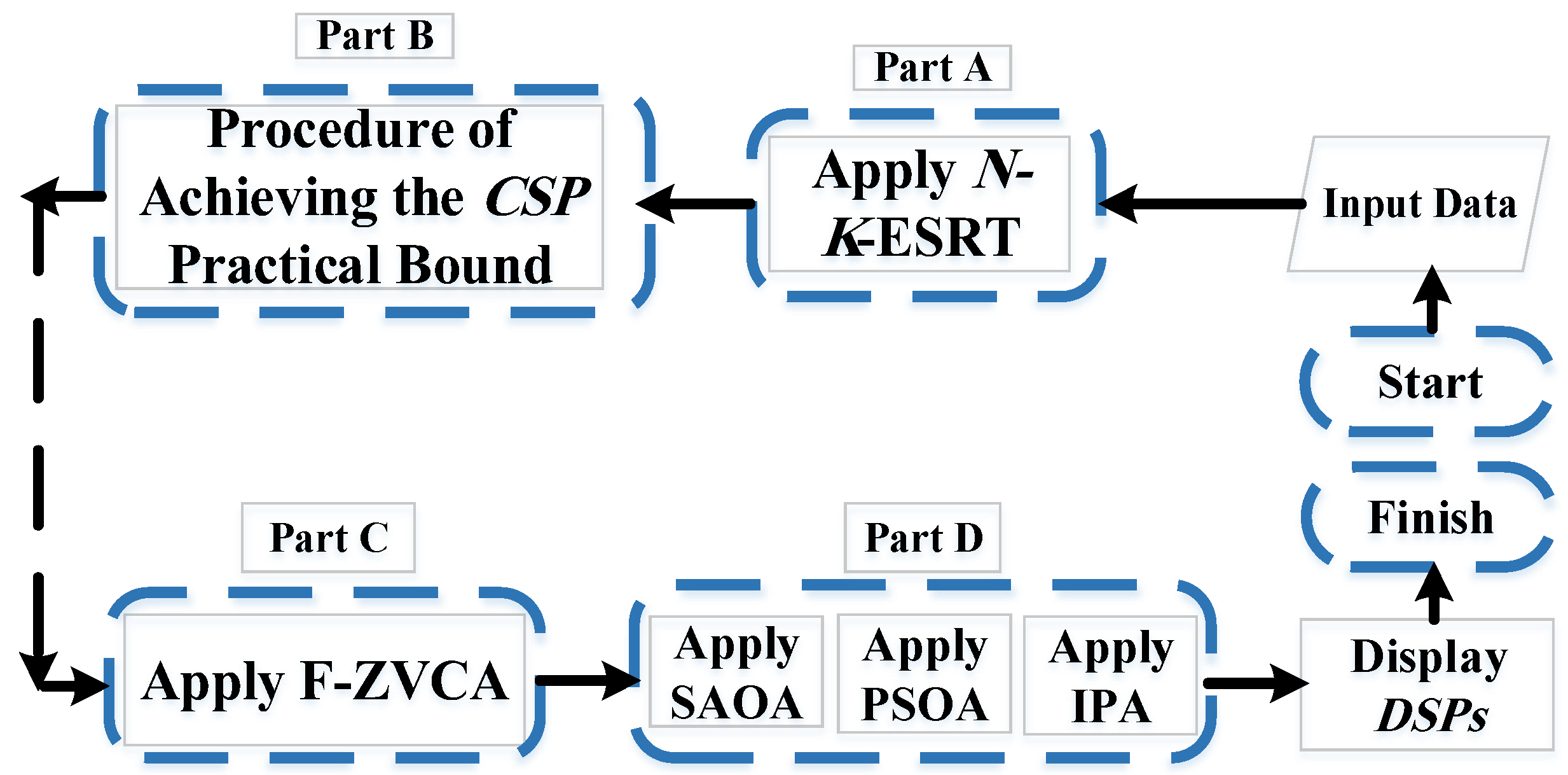
3. Protection Optimization Setting Problem

The POSP is divided into four parts, as shown in Figure 1. The N-K-ESRT as Part A (Section 3.1) is initially applied to N-2 contingencies, and the chosen contingencies are identified. After that, the limitations of CSP are determined by the procedure described in Part B (Section 3.2). Next, F-ZVCA is performed to group the findings of N-K-ESRT in Part C (Section 3.3). In conclusion, MOAs will optimize the values of DSPs as Part D (Section 3.4). Each part is described in depth below.

3.1. N-K Events Scale Reduction Technique

Professional standards mandate that microgrids be safeguarded against a single event, or N-1 contingency [39,40,41]. Nevertheless, it is conceivable that K events occurred simultaneously, which is alluded to as N-K contingencies. Technically, the POSP does not need to take into consideration the three or four simultaneous outages (K ≥ 3). This is due to the fact that the probabilities of these component failures are multiplied by each other, and the possibility of such occurrences is exceedingly low [42]. The incidence of N-2 contingencies results in the disconnection of critical industrial loads and a sharp rise in energy not supplied (ENS) [43,44,45]. In light of this, the POSP of DOCRs is assessed, considering N-2 events. However, managing N-2 contingencies is significantly more difficult due to their vast number, especially in large-scale systems. Accordingly, the N-K-ESRT is recommended as an innovative solution to this problem. Due to the construction of N-K-ESRT, the number of all N-2 probable events will greatly decrease. The N-K-ESRT puts all supposed outage-related equipment (lines, DGs, generators, etc.) into a subset. Next, the maximum and minimum voltage limits of each network’s bus are calculated for all N-2 outages. Following this, the process selects the N-2 outages that result in the highest and lowest voltages for each bus. Given that the amount of current flowing through a line is directly proportional to the voltage difference between its corresponding buses, this technique encompasses the entire spectrum of network currents for all N-2 events.

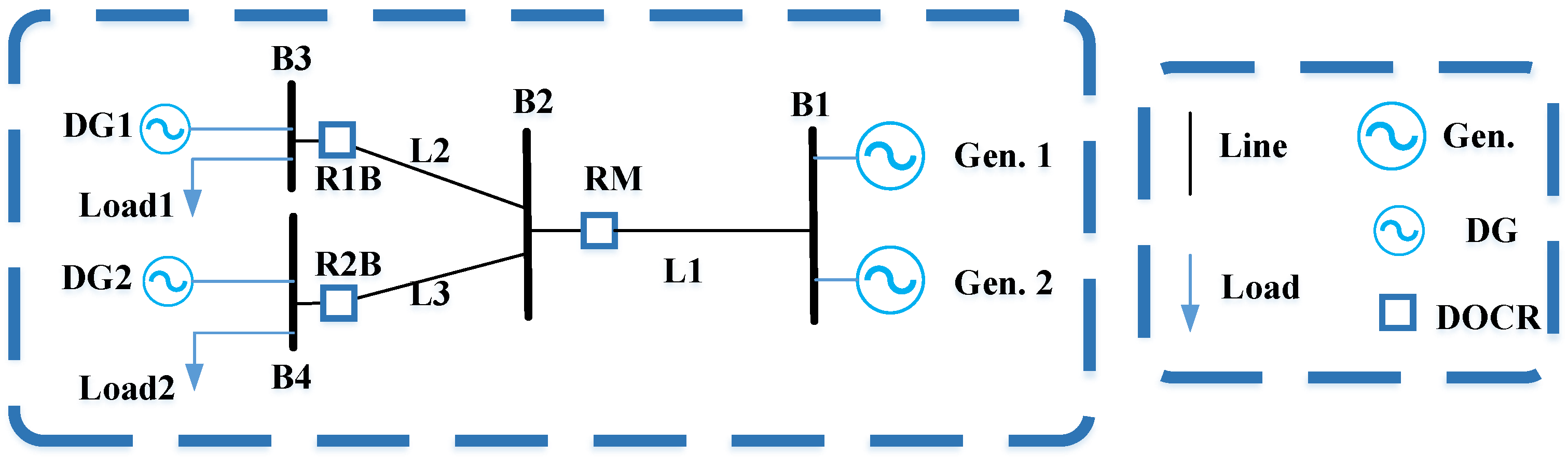
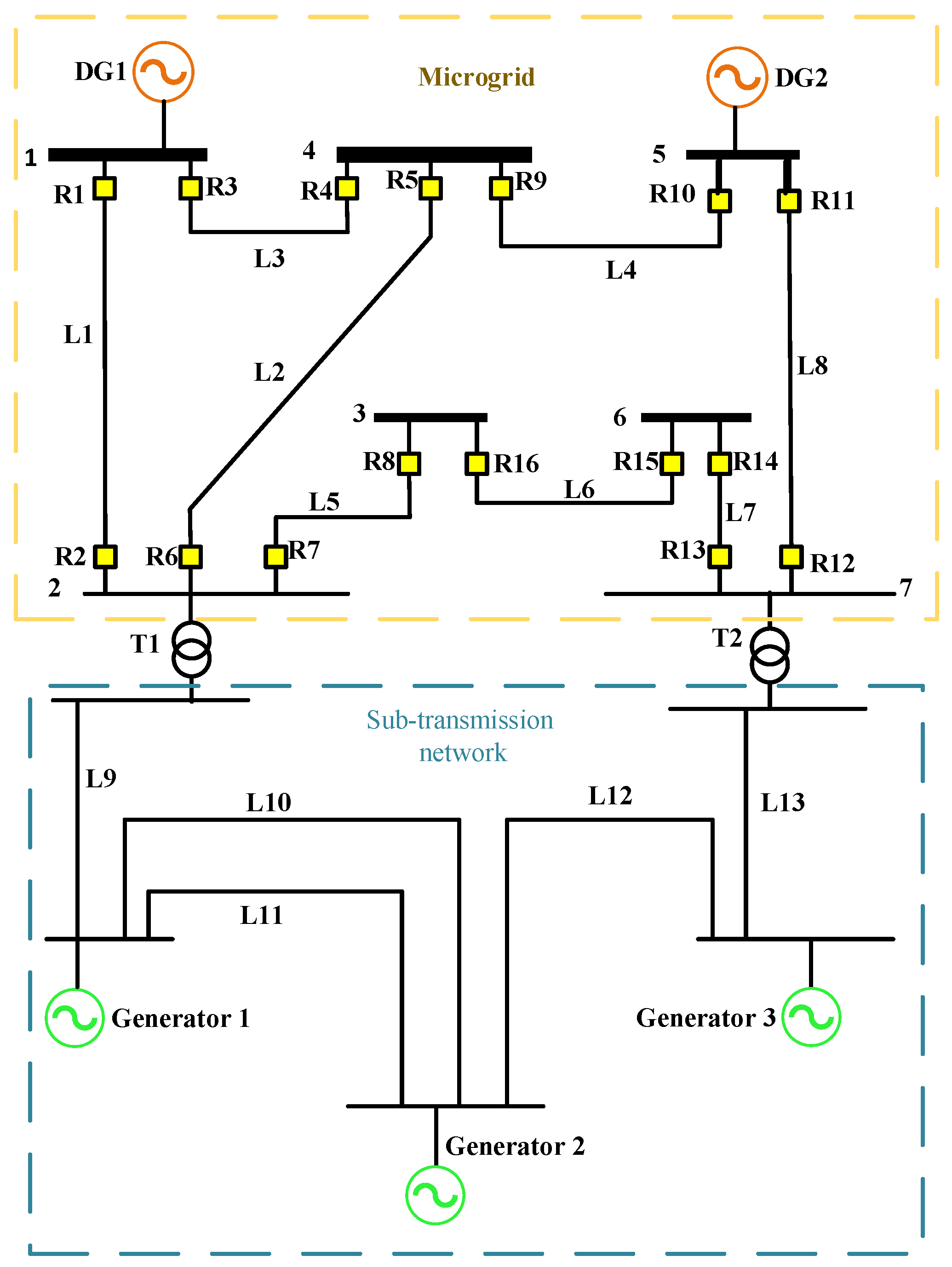
Consider Figure 2 as a sample network for judging this approach.

All anticipated equipment for N-2 contingencies in a subset consists of nine components, including DG1 and DG2, load 1 and load 2, lines (i.e., L1, L2, and L3), and generators (i.e., Gen. 1 and Gen. 2). In order to implement the intended technique, the earlier specified equipment must be taken out of service in two simultaneous events, and the voltage of the buses (i.e., B1, B2, B3, and B4) must be measured in each of these occurrences. For example, one of the N-2 events led to the lowest voltage value in B1, and another led to the highest voltage value in the same bus. The N-K-ESRT has picked these two occurrences as the chosen contingencies for B1. The POSP automatically applies this approach to each bus, resulting in eight occurrences based on (8) for the sample network’s buses (i.e., NU^ESRT equals two times the number of buses in the network under investigation). Rather, if all N-2 outages are considered, 36 occurrences (called OCC) will need to be investigated as (9) [46]. POSP is able to access the “maximum voltage violation study” for cascading events with the help of the Power Factory 15.1.7 DIgSILENT software. The result of this analysis reveals which of these 36 scenarios has the greatest and least noticeable impact on the network bus voltage. So, this method has led to a 75% decrease in the number of N-2 events in the sample network, which would help reduce the size of the problem and speed up the POSP. It should be emphasized that, with the rise of assuming equipment for N-2 events, this technique will be more beneficial than before.

$$\left\{N{U}^{ESRT}=〈{\displaystyle \sum _{NB=1}^{NAB}2\times NB}〉\right\}$$

(8)

$$\left\{OCC=〈\frac{N\text{!}}{(N-2)!\times 2}〉\right\}$$

(9)

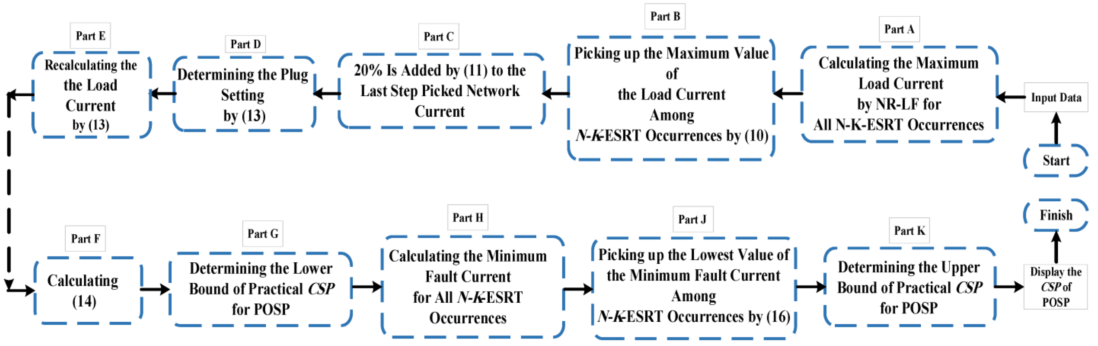
3.2. The Procedure of Achieving the CSP Practical Bound (PA-CSP-PB) for the POSP

To facilitate the description of this section, Figure 2 serves as the sample network (as depicted in the N-K-ESRT section), and Figure 3 (consisting of parts A–K) provides the flowchart of PA-CSP-PB. The idea of this section is to acquire the CSP practical range of R_M (shown in Figure 2) according to (6) and (7), which can be applied to the rest of the DOCRs. First, the maximum network current passing through the R_M is used to determine the least bound of (7) for the R_M. This is accomplished by employing the Newton–Raphson load flow (NR-LF) to compute the current flowing through L1 (seen in part A).

The picked current for the next part (part B) is the maximum current passing through the L1 ($I_{\mathit{Loadmax}}^{R_M}$) for all eight network configurations, which is attained by (10). As described in the preceding section, the N-K-ESRT identifies eight occurrences of two simultaneous outages. Subsequently, $I_{\mathit{Loadmax}}^{R_M}$ among these eight occurrences, one is chosen as the R_M’s maximum current. Additionally, (11) adds 20% to the $I_{\mathit{Loadmax}}^{R_M}$, named $I_{\mathit{Pickup}}^{R_M}$. This issue is due to the necessity of preventing a false trip caused by a maximum load current rather than a permanent fault (shown in part C). As seen in part D, (13) obtains the plug setting (${PS}_{}^{R_M}$) for the following approach, using (12) as an asset. The plug setting is the percent of R_M’s CT winding, which varies from 50% to 200% in 25% increments. The ratio between the primary (CTP) and secondary (CTS) windings of a CT is denoted by (12) and written as CTR. In accordance with PA-CSP-PB, the plug setting is rounded up and $I_{\mathit{Pickup}}^{R_M}$ is recalculated by (13) as part E. Next, the current flowing through the secondary side of the CT ($I_{CSP}^{R_M}$) is calculated using the formula (14) and is illustrated in part F. This current ($I_{CSP}^{R_M}$) is the same current that should be deemed the lowest bound in (7). Particularly, the relation specified in (15) will suffice as the CSP bound of POSP. Accordingly, the lower limit of (15) is the greatest value between $I_{\mathit{CSP}}^{R_M}$ and ${\mathit{CSP}}_{\min }^{}$(seen in part G). Selecting the maximum value at the lower limit of (15) is intended to prevent network power interruptions. The upper limit of (15) also represents the least value between ${\mathit{CSP}}_{\mathit{max}}^{}$ and $I_{\mathit{FCmin}}^{R_M}$. Note that the minimal short circuit current (i.e., $I_{\mathit{FCmin}}^{R_M}$) employed in the case studies is equivalent to the single-phase ground fault current stipulated by standard IEC 60909-2001 [47] (part H). Similar to the preceding process that established the lower limit of the CSP, the short circuit current value used in the next part is the lowest short circuit current among all N-K-ESRT’s topologies based on (16) and depicted in part J. The fault current determined by (16) is the maximum bound of (7). Now, the upper limit of (15) is the minimum value between the $I_{\mathit{FCmin}}^{R_M}$ and ${\mathit{CSP}}_{\mathit{max}}^{}$ (part K). Considering that the L1 should be rendered inoperable in the event of a short circuit, the minimum value was set at the upper limit of (15). The PA-CSP-PB will perform all the described steps for each relay. The PA-CSP-PB relations can be defined as:

$$\left\{I_{\mathit{Loadmax}}^{M,S}=\mathit{MAX}〈I_{\mathit{Loadmax}}^{M,1}{,I}_{\mathit{Loadmax}}^{M,2}\dots {,I}_{\mathit{Loadmax}}^{M,S}〉\right\}$$

(10)

$$\left\{I_{\mathit{Pickup}}^M=〈I_{\mathit{Loadmax}}^{M,S}\times 1.2〉\right\}$$

(11)

$$\left\{{\mathit{CTR}}^M=〈\frac{{\mathit{CTP}}^M}{{\mathit{CTS}}^M}〉\right\}$$

(12)

$$\left\{{\mathit{PS}}^M=〈\frac{I_{\mathit{Pickup}}^M}{{\mathit{CTP}}^M}\times 100〉\right\}$$

(13)

$$\left\{I_{\mathit{CSP}}^M=〈\frac{I_{\mathit{Pickup}}^M}{{\mathit{CTR}}^M}\times 100〉\right\}$$

(14)

$$\left\{〈{\mathit{MAX}(\mathit{CSP}}_{\mathit{min}}^{M,S}{,I}_{\mathit{CSP}}^M)\le {\mathit{CSP}}^{M,S}\le {\mathit{MIN}(\mathit{CSP}}_{\mathit{max}}^{M,S}{,I}_{\mathit{FCmin}}^{M,S}〉\right\}$$

(15)

$$\left\{I_{\mathit{FCmin}}^{M,S}=\mathit{MIN}〈I_{\mathit{FCmin}}^{M,1}{,I}_{\mathit{FCmin}}^{M,2}\dots {,I}_{\mathit{FCmin}}^{M,S}〉\right\}$$

(16)

3.3. Fuzzy Zero-Violation Clustering Algorithm

Multiple setting groups are a function of the utilized relays that permit the DOCRs to have several DSP groups, only one of which operates in the present grid structure [5,6,7,8]. To employ DOCR’s MSG, similar DSPs are placed in the right cluster using clustering algorithms. Given that there are four MSGs in DOCR, the N-K-ESRT must be divided into four clusters (or less than four clusters). Clustering is a mathematical technique for categorizing several similar data points into distinct groups [6]. As an innovative clustering algorithm, the F-ZVCA groups all topologies obtained by N-K-ESRT into separate clusters using the procedure outlined below. The concept of F-ZVCA comes from k-means clustering, fuzzy C-means clustering, and POSP trial and error.

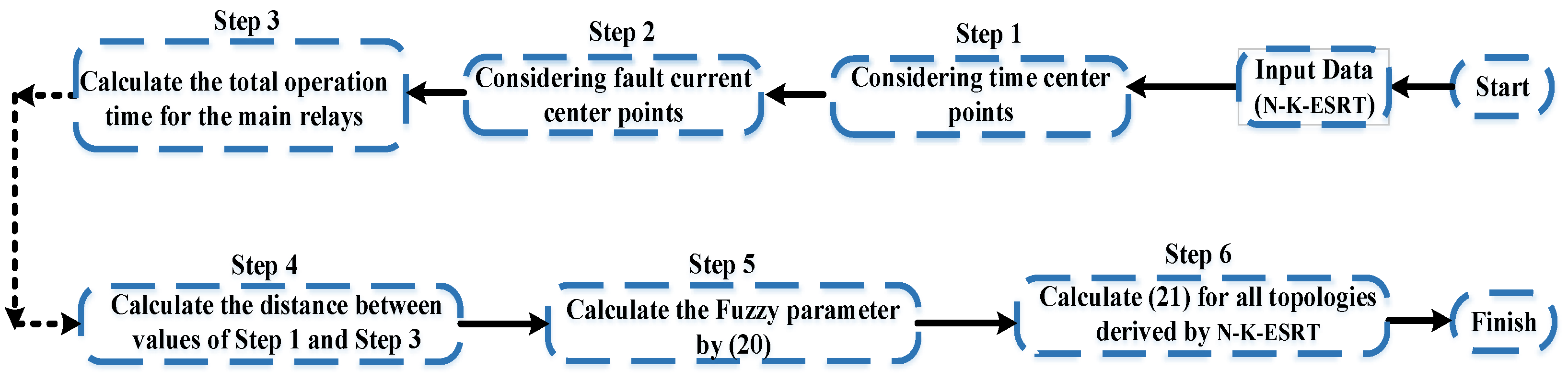
Assigning each topology to its appropriate cluster involves the following six steps, which are shown in Figure 4:

Step 1: Initially, time center points are randomly considered as the centers of the clusters (OT^C1, OT^C2, OT^C3, and OT^C4). These center points indicate the total operating time (OT) of the network’s primary relays. For instance, OT^C1 is identified as the time center point for the “C1” cluster (i.e., cluster 1).

Step 2: Secondly, fault current center locations designated ${\mathsf{\lambda }}_{}^C$(including ${\mathsf{\lambda }}_{}^{C1},{\mathsf{\lambda }}_{}^{C2},{\mathsf{\lambda }}_{}^{C3},$ and ${\mathsf{\lambda }}_{}^{C4}$) are picked at random as supplementary cluster centers. These center points reflect the total fault current ratio between the main DOCRs and their backup relays. In this particular case, the fault current centroid point of “C2” (i.e., cluster 2) is shown as ${\mathsf{\lambda }}_{}^{C2}$.

Step 3: Subsequently, the total operation time of the main relays is decided based on (17) for all derived topologies (OT^S1, OT^S2… etc.) with the help of (1) and the default TSMP = 1, and CSP = I_CSP. For example, OT^S3 signifies the total operation time of the main DOCRs for the “S3” topology.

Step 4: Fourth, using (18), the distance of OT^S1 from all time center points (i.e., OT^C1, OT^C2… etc.) is determined and designated as DOT^S1-C1, DOT^S1-C2, … This procedure is done for each resultant topology (i.e., DOT^S2-C1… DOT^S3-C1…).

Step 5: Using the formula in (19), a fuzzy parameter denoted $\mathsf{\omega }{\mathsf{\lambda }}_{}^{S-C}$ is derived by (20). Equation (19) signifies the average ratio between the fault current of the primary DOCR and their backup relays. ${\mathsf{\lambda }}_{}^S$ is computed for any topologies coming from N-K-ESRT. In essence, (19) demonstrates that the fluctuations in the short-circuit level were significant for each topology; presumably, that topology should have a higher probability of being conveyed.

(Note: The resultant topologies should be more likely to be clustered together when the $\mathsf{\omega }{\mathsf{\lambda }}_{}^{S-C}$ values are closest to each other among all ones.)

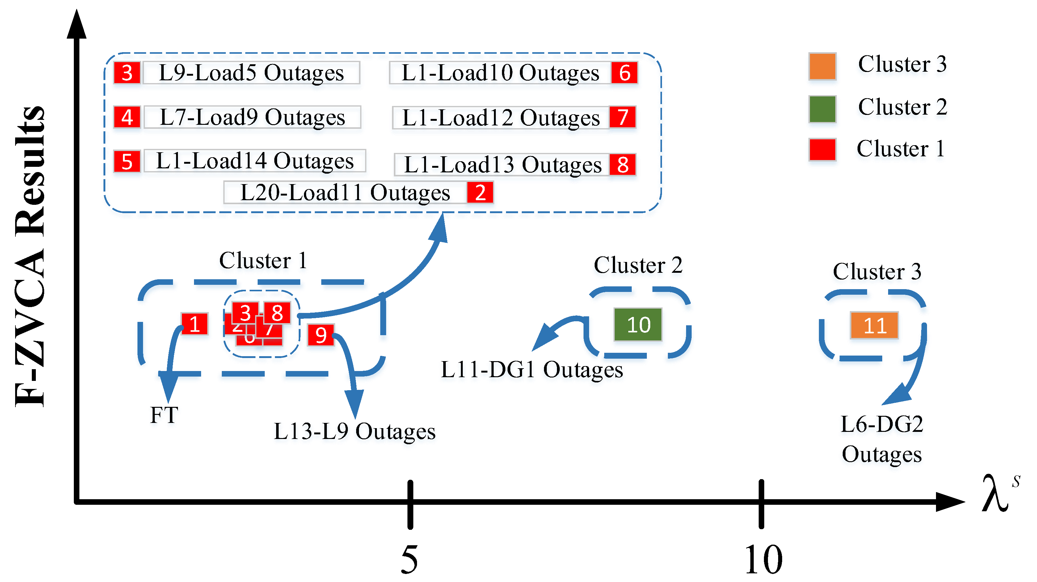
Step 6: Equation (21) is determined between each derived topology and the clusters using (20) and (18). Among the values obtained for topology ‘S1’, including:$D\mathsf{\omega }$^S1-C1, $D\omega$^S1-C2, $\dots ,$ topology ‘S1’ is allocated to the cluster with the smallest $D\omega$^S-C value. Lastly, steps 1 through 6 are repeated until the clusters’ constituents are no longer altered.

The F-ZVCA will therefore exhibit its results if the POSP has no miscoordination across all clusters. If miscoordination has occurred, F-ZVCA relocates the specific topology to a different cluster. As stated previously, the specified topology must be transmitted from its cluster to another cluster with the maximum possible value of (21). This topology should be transmitted to the succeeding cluster if (19) has the greatest value deviation compared to the other topologies generated by N-K-ESRT. The relationships associated with F-ZVCA can be described as follows:

$$\left\{O{T}^S={\displaystyle {\sum }_{M=1}^Q〈\frac{0.14\times 1}{((\frac{I_{FC}^{M,S}}{I_{CS{P}^{M,S}}}{)}^{0.02}-1)}〉}\right\}$$

(17)

$$\left\{DO{T}^{S-C}=〈\left|O{T}^S-O{T}^C\right|〉\right\}$$

(18)

$$\left\{{\lambda }_{}^S=Avg〈{\displaystyle \sum _{M,\mathit{JB}}^{}\frac{I_{\mathit{FC}}^{M,S}}{I_{\mathit{FC}}^{\mathit{JB},S}}}〉,\forall (M,JB),\forall S\right\}$$

(19)

$$\left\{{\mathsf{\omega }\mathsf{\lambda }}^{S-C}=〈\frac{\left|{\mathrm{\lambda }}^S-{\mathrm{\lambda }}^C\right|}{{\mathrm{\lambda }}^C}〉\right\}$$

(20)

$$\left\{{D\mathsf{\omega }}^{S-C}=〈\mathsf{\omega }{\mathsf{\lambda }}^{S-C}\times DO{T}^{S-C}〉\right\}$$

(21)

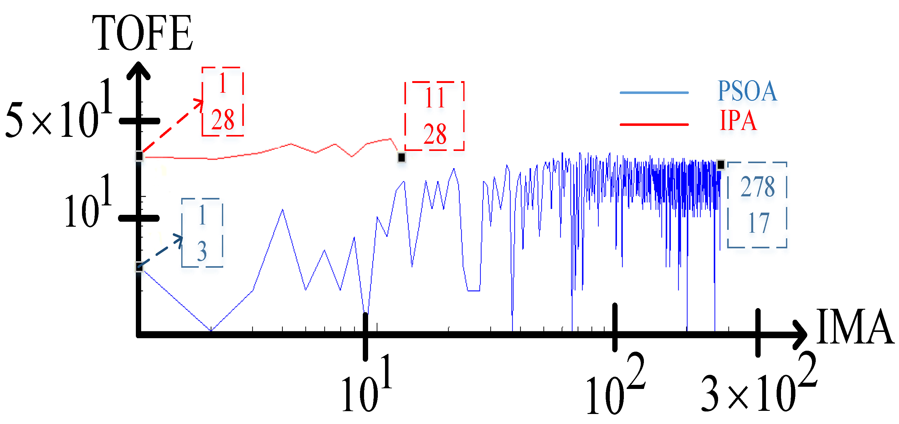
3.4. Meta-Heuristic Optimization Algorithms

After the N-K-ESRT and F-ZVCA reduce the dimensions of the POSP, the DPSs are produced employing three MOAs, encompassing IPA, SAOA, and PSOA. The IPA handles both vastness and spread as well as smallness and concentration problems and may be retrieved from either NaN or Inf results [48]. Besides, SAOA is a technique for answering both constrained and unconstrained optimization issues. Accepting poorer solutions throughout the optimization procedure while retaining the ability to escape local points is a distinguishing feature of SAOA [22]. On the other hand, PSOA is highly valuable for nonlinear programming problems and has the potential to substantially optimize local search. Refer to [22,48,49] for details on the IPA, SAOA, and PSOA, respectively.

4. POSP Setup

4.1. The Assumption about the POSP

Owing to the fact that the FT of the network is a stable state of the power grid and the power network is continually fluctuating between the FT and event-derived topologies, the FT has been deemed the default in all clusters. After trial and error in the problem-solving procedure, it has been proven that the I_CSP is always higher than the CSP_min and lower than the I_FCmin in all evaluated cases. Nevertheless, as examined and validated by Noghabi et al. [34], including both decision variables of DOCRs in the cycle of optimization algorithms merely slows down the convergence process of the problem. Therefore, the CSP is equivalent to the I_CSP, which will be produced by using PA-CSP-PB. As a result, the CSPs are the same across all clusters and are not cluster-dependent. The end criteria for POSP are OF’s tolerance and MOA’s execution time (MET). The OF’s tolerance is presumed to be 1 × 10⁻¹⁶, and the maximum limit of MET is set to 100 s, resulting in more accurate findings [50]. This section additionally provides the average tripping time (ATT), the ATT for one relay (ATTO), the maximum tripping time (MTT), the overall TSMP (O-TSMP), and the iteration of MOAs (IMA) to aid comprehension of the POSP. Furthermore, logarithmic indices have been utilized on numerous vertical and horizontal axes of the figure obtained from POSP in order to enhance the distance portrayal and coherence of the paper’s figures.

4.2. N-K-ESRT and F-ZVCA Results: IEEE Std. 399-1997 System

As observed in Figure 5, the IEEE Std. 399-1997 network is made up of 19 buses (B1, …, B19), 20 lines (L1, …, L20), 14 loads (Load1, …, Load14), 26 relays (R1, …, R26), and 1 external grid (EX). This industrial network is connected to the EX through two 69 KV/13.8 KV transformers (T1 and T2) [51]. In particular, this system is linked to two DG units with capacities of 15.6 MVA and 12.5 MVA for DG1 and DG2, respectively. This network is scheduled to contain 39 pieces of equipment for N-2 events (including all DGs, loads, lines, transformers, and Ex). There are 741 cases of N-2 events, according to (9). However, in accordance with

Table 2. Results of N-K-ESRT for the IEEE Std. 399-1997 system.

Bus	B1		B5		B6		B7		B8		B9		B10		B 11
	LB	UB	LB	UB	LB	UB	LB	UB	LB	UB	LB	UB	LB	UB	LB	UB
EV	0.95	1	0.94	1	0.94	0.99	0.94	1	0.94	0.99	0.94	1	0.94	0.99	0.94	1
VFT	1		0.99		0.99		0.99		0.99		0.99		0.99		0.99
EN	L11-DG1	FT	L11-DG1	L13-L9	L11-DG1	FT	L11-DG1	FT	L11-DG1	FT	L11-DG1	FT	L11-DG1	FT	L11-DG1	L9-Load5
Bus	B 12		B13		B14		B15		B 16		B17		B18		B19
	LB	UB	LB	UB	LB	UB	LB	UB	LB	UB	LB	UB	LB	UB	LB	UB
EV	0.94	0.99	0.94	1	0.94	0.99	0.94	1	0.94	0.99	0.95	1	0.95	1	0.95	1
VFT	0.99		0.99		1		0.99		0.99		0.99		0.99		0.99
EN	L11-DG1	FT	L11-DG1	L7-Load9	L11-DG1	FT	L11-DG1	L1-Load10	L11-DG1	L20-Load11	L6-DG2	L1-Load12	L6-DG2	L1-Load13	L6-DG2	L1-Load14

, only eleven occurrences are investigated by N-K-ESRT, which reduces the size of the POSP by 98.651%. Due to the availability of 16 buses on the distribution part of the Example St. 399-1997 network, the N-K-ESRT ought to provide 32 cases based on (8). Due to the frequent bus-related events (illustrated in Table 2 in the EN row), the N-K-ESRT results are limited to 11 modes as opposed to 32 modes. Table 2 indicates that the voltage of fixed topology (VFT) for bus 5 is 0.99 PU. The VFT increases to the event voltage (EV) of 1 PU following the outages of L13-L9 (i.e., simultaneous outages for lines 13 and 9). In contrast, the VFT decreases to 0.94 PU as a result of the outages of lines 11 and DG1 (event name: EN). Notably, the aforementioned contingencies (L13 and L9 outages, L11 and DG1 outages) result in the lower (LB) and upper (UB) bounds of voltage ranges for bus 5 among all N-2 occurrences. After defining the chosen contingencies by N-K-ESRT, the F-ZVCA is utilized in order to group these contingencies. As a result of F-ZVCA, Figure 6 depicts the clustering of the N-2 contingencies into three clusters (Clusters 1–3). The maximum number of occurrences is allocated to cluster 1, which has nine topologies, indicating that these topologies are closer in terms of the short-circuit current based on (19). In addition, cluster 2 and cluster 3 only account for a single N-2 contingency, which includes L11-DG1 and L6-DG2 outages, respectively.

4.3. Simulation Results: IEEE Std. 399-1997 System

The SAOA and PSOA are not converged for the IEEE Std. 399-1997 system. The impediment clusters in the trend of convergence of SAOA and PSOA are clusters 3 and 1, respectively, which cause the POSP to be implemented in a way that is not coordinated. Given that the POSP is worthless if even a single DOCR of the clusters causes failure (i.e., one miscoordination is sufficient to render the POSP ineffective). In greater detail, in the case of miscoordination, the penalty variable (i.e., η) causes the OF to grow overly large, resulting in the POSP failing to converge. Despite the aforementioned algorithms, IPA’s results among all three clusters are error-free, ending in a flawless convergence of POSP. As depicted in Figure 7,

Table 3. DSPs for the IEEE Std. 399-1997 system reached by IPA.

Relay		R1	R2	R3	R4	R5	R6	R7	R8	R9	R10	R11	R12	R13
CSP		1.8	1.8	1.8	1.8	1.4	1.4	1.4	1.4	1.4	2	2	1.6	1.6
TSMP	Cluster 1	0.39	0.427	0.399	0.427	0.691	0.381	0.49	0.847	0.49	0.876	0.509	0.595	0.529
	Cluster 2	0.392	0.454	0.391	0.456	1	0.583	0.84	0.964	0.05	0.994	0.052	0.113	0.667
	Cluster 3	0.471	0.05	0.471	0.05	0.557	0.999	0.356	0.45	0.05	0.667	0.05	0.285	0.508
Relay		R14	R15	R16	R17	R18	R19	R20	R21	R22	R23	R24	R25	R26
CSP		1.6	1.6	1.6	1.6	1.4	1	1	1.8	1.4	1.4	0.8	1.8	1.6
TSMP	Cluster 1	0.645	0.973	0.429	0.516	0.178	0.491	0.492	0.462	0.978	0.354	0.475	0.475	0.475
	Cluster 2	0.142	0.91	0.053	0.488	0.08	0.285	0.267	0.276	0.488	0.488	0.292	0.266	0.278
	Cluster 3	0.388	0.829	0.393	0.482	0.051	0.649	0.05	0.392	0.482	0.337	0.393	0.361	0.366

and

Table 4. Results of the IEEE Std. 399-1997 system reached by IPA.

System	O-TSMP	MTT	ATT	ATTO	OF	MET	IMA	TOFE
Cluster 1	14.015	28.332	28.229	1.085	314	1.8	20	715
Cluster 2	11.281	25.892	25.892	1.078	240	8.1	85	3010
Cluster 3	10.147	21.22	21.22	0.884	184.5	1.8	19	687

, the optimized OFs of IPA for clusters 1, 2, and 3 are 314, 240, and 184.5, with 20, 85, and 19 IMA, respectively. Table 3 lists the DSPs accessed by IPA for all three clusters of the IEEE Std. 399-1997 system. It is crucial to highlight that optimal DSPs will enable the propensity of OFs to converge. This indicates that changes in DSPs have a direct impact on OF values. As seen in Table 3 and mentioned before, CSPs are the same throughout all clusters and are not cluster-dependent. Since each cluster has a specific set of limitations associated with its system topologies, the TSMPs are not identical between all clusters in the same way that CSPs are. According to Table 4, the O-TSMP (MTT, ATT, and ATTO) best achieved by IPA for clusters 1, 2, and 3 is 14.015 s (28.332 s, 28.229 s, and 1.085 s), 11.281 s (25.892 s, 25.892 s, and 1.078 s), and 10.147 s (21.22 s, 21.22 s, and 0.884 s), respectively.

It is clear that cluster 1 has higher values for OF, O-TSMP, MTT, ATT, and ATTO than clusters 2 and 3. In light of this, the POSP is handled by the greatest number of topologies allocated to cluster 1 (seen in Figure 6), resulting in a more complex problem for cluster 1 than the other clusters. For extra information, POSP must be performed for each of the nine topologies assigned to cluster 1, and the aforesaid limitation must be met for all of them. In terms of short circuit level, the POSP of clusters 2 and 3 is much more relaxed than that of cluster 1. This advantage is exacerbated by the fact that clusters 2 and 3 cover just one of the N-2 outages, yielding the smallest influence on fluctuations in short-circuit current. Therefore, cluster 1 has the longest tripping time relative to the other clusters due to the fact that the fault current is inversely proportional to the DOCR’s tripping time based on (2). In addition, IPA’s METs for clusters 1, 2, and 3 are 1.8 s, 8.1 s, and 1.8 s, respectively. These MET are extremely fast computation times that are appropriate for solving the POSP. Moreover, the total objective function evaluation (TOFE) determined by IPA for clusters 1, 2, and 3 is 715, 3010, and 687, as displayed in Figure 8 and Table 4. The TOFE refers to the number of OF evaluations throughout each iteration. For deeper inquiry, and as seen in Figure 8, cluster 1 has 31 TOFE in the first iteration and 50 TOFE in the last iteration. It should be noted that the MET of cluster 2 is 4.5 times longer than those of clusters 1 and 3, culminating in the TOFE of cluster 2, which is much bigger than those of clusters 1 and 3.

4.4. Simulation Results: TESKO2 System

An industrial radial feeder designated as the TESKO2 feeder is represented in Figure 9. Actually, one of the sub-transmission substation’s (which is considered an EX) outgoing feeders is the TESKO2 feeder, which is situated in northwest Iran.

This system has three DGs (DG_a, DG_b, and DG_c) with a capacity of 2.2 MVA, five lines (L1, …, L5), three loads (Load_a, Load_b, and Load_c), and ten DOCRs (R_a, …, R_X). In the TESKO2 network, the presumed equipment for N-2 events consists of 12 components, including all loads, synchronous machines, and lines, of which only five topologies are analyzed as N-K-ESRT. The repercussions of N-K-ESRT have involved Load_a-Load_b outages, L1-L2 outages, DG_a-DG_c outages, DG_a-DG_b outages, and FT. If the F-ZVCA is employed, it is expected that all NU^ESRT occurrences are kept within a single cluster with zero miscoordination.

Therefore, the paucity of these topological quantities is the reason for the absence of clustering in this network. Despite the former case study, the TESKO2 system has converged across all MOAs (SAOA, PSOA, and IPA). As demonstrated in Figure 10 and

Table 5. Results of the TESKO2 system reached by MOAs.

Relay		Ra	Rb	Rc	Rd	Re	Rf	Rg	Rh	Ri	Rx	All Relays
CSP		1.8	1.8	1.8	1.8	1.4	1.4	1.4	1.4	1.4	2	O-TSMP	ATT	MTT	ATTO	OF	MET	IMA
TSMP	IPA	0.465	0.407	0.418	0.572	0.41	0.409	0.413	0.571	0.998	0.573	5.236	9.432	12.284	0.943	1300.8	1.1	11
	SAOA	0.128	0.067	0.389	0.486	0.216	0.067	0.266	0.259	0.547	0.366	2.796	6.915	11.198	0.691	555.9	100	1777
	PSOA	0.05	0.146	0.185	1	0.15	0.05	0.214	0.17	0.311	0.246	2.522	4.562	5.863	0.456	262.9	25.5	263

, the converged OF of SAOA, PSOA, and IPA is 555.94 (with 1777 IMA), 262.97 (with 263 IMA), and 1300.85 (with 11 IMA), respectively. Additionally, Table 5 reveals the findings for MOAs’ DSPs. In comparison to the earlier case study, it is anticipated that the ATT, ATTO, MTT, and O-TSMP will be attained with lower values for the TESKO2 system. The TESKO2 grid is a radial network, and as a result, the POSP limitations are far less severe than they are for the IEEE Std. 399-1997 system. As indicated in Table 5, the ATT attained by SAOA, PSOA, and IPA is 6.915 s, 4.562 s, and 9.432 s, respectively. As a result, the PSOA is the optimal solution in terms of average operation time for one DOCR, with a value of 0.456 s as ATTO. The O-TSMP values acquired by PSOA and IPA are 2.522 s and 5.236 s, respectively, which are the lowest and highest values ever observed. The IPA method is implemented disappointingly in terms of MTT and ATT, with values of 12.284 s and 9.432 s, respectively. Nevertheless, the algorithm with the lowest MET is the IPA, whose MET is faster than other MOAs. The MET achieved by IPA, PSOA, and SAOA is 1.1 s, 25.5 s, and 100 s, respectively. It should be emphasized that the upper bound of MET and the function tolerance are the end criteria for SAOA and IPA, respectively.

Consequently, it can be stated that the IPA and PSOA have been deemed the privileged MOAs for the TESKO2 feeder in terms of MET and ATTO, respectively (Figure 11 represents the TOFE of these algorithms). As shown in Figure 11, the TOFE values for IPA and PSOA are 378 and 3527, respectively. Given that PSOA’s MET is 23.18 times longer than IPA’s (mentioned in Table 5), the TOFE of PSOA is dramatically higher than that of IPA. Moreover, it can be pointed out that the TOFE of IPA acquired for the IEEE Std. 399-1997 system has a growing trend compared to the TESKO2 feeder, which is due to the fact that the IEEE Std. 399-1997 network is notably more looped than the TESKO2 grid. In looped systems, it is considerably more challenging to satisfy TSMP and coordination constraints than in radial networks. Because of this concern, IMA and MET rise significantly, forcing meshed networks to have a higher TOFE than radial networks.

4.5. Simulation Results: IEEE 14 Bus System

In this section, the IEEE 14 bus system will be considered to compare its results with four studies, including Refs. [1,5,6,12]. The technical details of the equipment for the IEEE 14 bus system are provided in Appendix C.

Here, only the findings of IPA for the IEEE 14 bus system are provided. The IEEE 14 bus network is comparable to the IEEE Std. 399-1997 and is more looped as a microgrid (the SAOA and PSOA are not converged in the IEEE Std. 399-1997 system). On the other hand, only IPA’s outcomes are flawless, ending in a convergence of the problem for the IEEE 14 bus system.

All 20 components of the IEEE 14 bus system (illustrated in Figure 12) are susceptible to failure. They consist of five synchronous machines (two DGs and three generators), thirteen lines (L1, …, L13), and two transformers (T1 and T2). However, only the equipment failures of the microgrid portion of the IEEE 14 bus system (shown in Figure 12) are considered in the studies referenced. According to (9), the IEEE 14 bus system’s N-2 contingencies result in 190 events. Despite this, as shown in

Table A27. The results of N-K-ESRT for the IEEE 14 bus system.

Bus		EV	VFT	EN
Bus 1	UB	1.314	1.104	L1-L3
	LB	1.058		L2-DG1
Bus 2	UB	1.177	1.070	Generator1-T1
	LB	1.070		FT
Bus 3	UB	1.187	1.087	Generator1-L8
	LB	1.087		FT
Bus 4	UB	1.269	1.092	L1-L3
	LB	1.058		DG1-DG2
Bus 5	UB	1.301	1.113	L3-L6
	LB	1.051		T1-T2
Bus 6	UB	1.151	1.075	Generator1-T2
	LB	1		T1-T2
Bus 7	UB	1.150	1.078	Generator1-T2
	LB	1.078		FT

(provided in Appendix C), only eleven events are investigated as selected contingencies based on N-K-ESRT findings. It should be noted that the repeated contingencies for each bus can reduce the results of the N-K-ESRT obtained by (8). It should be noted that if the N-K-ESRT is not deployed on the POSP, it will not be possible to verify all of these topologies (i.e., 190 events), as calculating the setting parameters of DOCRs for each one is a time-consuming and laborious task.

Table 6. Time results of previous studies compared to the proposed method of this paper in the IEEE 14 bus system.

STATE	The Proposed Method of This Paper without N-K-ESRT	The Proposed Method of This Paper with N-K-ESRT	[1]	[5]	[6]	[12]
1	TT = 7.765, O-TMSP = 2.013	TT = 7.765, O-TMSP = 2.013	TT = 8.366	TT = 14.062	-	TT = 11.058
2	ATT = 15.125, O-TMSP = 4.321	ATT = 12.598, O-TMSP = 3.487	-	ATT = 19.969	O-TMSP = 10.48	-
3	ATT = 20.213, O-TMSP = 6.558	ATT = 18.517, O-TMSP = 5.771	ATT = 49.783	-	-	-
4	-	ATT = 21.098, O-TMSP = 6.884	-	-	-	-

- stands for no data.

displays the tripping time (TT), ATT, and O-TSMP of all mounted DOCRs in the IEEE 14 bus system. These results are provided for various network topologies (four states), the methodology presented in this paper, and the referenced studies. Both ATT (or TT) and O-TSMP are provided for the proposed method of this paper; however, some columns in Table 6 are kept unfilled because only the results of these studies are presented. Four states are shown to be implemented on the IEEE 14 bus system in this table, including “FT” (state 1), “FT and N-1 contingency” (state 2), “FT, N-1 contingency, and island mode” (state 3), and “N-2 contingencies” (state 4). Additionally, the findings of the method described in this paper are specified both with and without N-K-ESRT for easy comparison and taking decisions regarding the approach to the problem. As indicated previously, the large number of topological states resulting from N-2 contingencies makes it impossible to implement this type of event without N-K-ESRT.

All four state outcomes demonstrate that the method proposed in this paper (even without N-K-ESRT) is markedly superior to those described in the aforementioned papers. The TT values of state 1, obtained by “the proposed method of this paper”, [1], [5], and [12], are 7.765 s, 8.366 s, 14.062 s, and 11.058 s, respectively. First, it should be noted that in this state (state 1 = fixed topology), ATT, N-K-ESRT, and F-ZVCA are meaningless (since there is only one topology), and the results of this paper are identical with or without N-K-ESRT.

The sole consequence of this state is the convergence of the optimization algorithm. State one’s findings indicate that the algorithm presented in this paper (IPA) and the parameters applied to it, as well as the objective function of the problem, worked well relative to other studies. For state 2, the procedure presented in this paper delivers the greatest results compared to the literature reviewed. The method proposed in this paper obtains an ATT of 15.125 s without N-K-ESRT and 12.598 s with N-K-ESRT, demonstrating the capability of N-K-ESRT. In addition, the O-TSMP value of the method presented in this paper without N-K-ESRT (4.321 s) is significantly lower than the value mentioned in [6] (10.48 s). The ATT determined by [1] for state 3 is 49.783 s, which corresponds to an operating time of 3.111 s per DOCR (because of the placement of sixteen DOCRs in the IEEE 14 bus system). However, the offered method of this paper with N-K-ESRT (18.517 s) and without N-K-ESRT (20.213 s) acquires the best results in state 3. Each relay’s operating time (without N-K-ESRT) is 1.157 s, which is 1.95 s faster than [1]. It deserves to be noted that the island mode is one of the N-2 outage modes (T1 and T2 outages) that leads to an exponential increase in the ATT. In the end, the approach outlined in this paper attains an ATT of 21.098 s for the N-2 contingencies, which is employed by N-K-ESRT.

Finally, it can be concluded that IPA is the only algorithm that has produced stability in the meshed systems (including IEEE 14 bus and IEEE Std. 399-1997 networks). It was straightforward to determine whether the IPA was superior to other algorithms in terms of decreasing the time required for relays to trip and accelerating the rate of convergence of the POSP. In addition, an additional advantageous feature of the IPA is its extremely rapid MET. On the other hand, PSOA is recommended for the TESKO2 network due to its superior performance in comparison to the other MOAs.

5. Conclusions

The POSP of the DOCRs in light of the unpredictability of the power systems is one of the most important issues of the past decade. In addition, a number of references have investigated the optimal protective strategies for microgrids, taking into account various configurations, and a small number of studies have concentrated on all N-1 contingency topologies. However, in none of the available references for the protection setting problem of DOCRs, there were no signs of solving techniques for the implementation of the N-2 contingencies in POSP. This paper suggests N-K-ESRT in an effort to lower the scale of N-2 events. Then, F-ZVCA serves to categorize these occurrences. Ultimately, PA-CSP-PB and MOAs (SAOA, PSOA, and IPA) are utilized to acquire the DOCRs’ DSPs. IPA is the only algorithm in the IEEE Std. 399-1997 and IEEE 14 bus networks that has contributed to convergence. The functionality of the IPA in this looped network in terms of DOCR’s operating speed and the convergence of the OF were effectively assessed. In addition to the convergence of the OF, another major advantage of the IPA is its extreme MET, as all case studies demonstrate. For the TESKO2 grid, the PSOA is considered to be the most effective MOA in terms of relay operation time. In particular, the tendency for the IPA in the looped systems to converge demonstrates that the F-ZVCA works well. It should be highlighted that the failure of convergence in one of the clusters will lead to a shortage of coherence in POSP. Thus, in the event of inadequate coordination, a malfunction ensues, and the network does not maintain its stable level, contributing to interruptions in load or cascading failures. Yet, this issue can be resolved by incorporating concurrent contingencies into the POSP of DOCRs.