Spatiotemporal Characteristics of Agricultural Production Efficiency in Sichuan Province from the Perspective of “Water–Land–Energy–Carbon” Coupling

Abstract

Maintaining low carbon levels is an important strategy to minimize the levels of carbon emissions globally, and utilization of energy in agricultural production activities is one of the major sources of carbon emissions. Promoting carbon reduction in agricultural production is a key method to achieve “carbon neutrality and carbon peaking”. This article established an input–output index system for evaluating agricultural production efficiency from the “water, land, energy and carbon” dimensions, and then used the super-efficient SBM model to calculate the value of agricultural production efficiency. The article combined the Malmquist index and spatial autocorrelation method to explore the spatiotemporal characteristics of agricultural production efficiency in Sichuan Province. Finally, this article analyzed the factors that affect agricultural production efficiency in Sichuan Province. The research results indicated that: (1) Agricultural carbon emissions in Sichuan Province decreased from 2011 to 2020, and agricultural carbon emissions in the eastern region were higher than the western region. (2) The agricultural production efficiency in Sichuan Province was generally above 0.88, with fluctuations observed from 2011 to 2020. Increase in agricultural production efficiency in the region was highly correlated with advances in technological progress. The spatial distribution of agricultural production efficiency exhibited an opposite trend to agricultural carbon emissions, and Moran’s I index was approximately 0, indicating a relatively random spatial distribution. (3) Analysis of influencing factors showed that the urbanization rate was inversely proportional to agricultural production efficiency, and the level of agricultural economic development was directly proportional to agricultural production efficiency. The agricultural production efficiency analysis model established in this article provides key information for developing policies to improve agricultural production efficiency and provides a basis for the practical promotion of low-carbon agricultural production in Sichuan Province. The paper provides a reference to develop strategies to achieve the regional “double carbon” goal.

1. Introduction

Global climate change poses a major threat to human life, and several countries have proposed “low carbon emission and carbon neutrality” as an essential strategy to achieve zero carbon emission [1]. Several countries have developed strategies to reduce carbon dioxide emissions and achieve carbon neutrality. Utilization of energy during agricultural production is one of the major sources of carbon emissions, accounting for 10–12% of the total amount of carbon emission globally [2]. Therefore, it is imperative to effectively control the level of carbon emissions during agricultural production.

Agricultural carbon emissions (ACE) refer to the total amount of carbon emission associated with agricultural activities. Several studies on ACE have been conducted from various perspectives, such as the various emission sources, methods used to determine carbon emission level and exploring carbon emission levels using different research objects. ACE are derived from inappropriate burning and utilization of chemical fertilizers, pesticides, agricultural plastics, irrigation, agricultural machinery and crop stalks. This type of carbon emission is mainly caused by human behaviors [3,4,5]. ACE are mainly evaluated based on the characteristics of crop growth, climate conditions and land. Soil utilization and the change of soil structure are major factors that directly affect ACE, as they contribute to generation of carbon emissions directly from the environment [6,7]. It is challenging to reduce the level of carbon emissions caused by the environment. Therefore, most scholars conduct research from the perspective of ACE that are not directly resulting from the environment.

Climate change, shortage of water and land resources and the energy crisis are key challenges that should be addressed. Recent studies on agricultural production efficiency (APE) proposed a new perspective, which involves inclusion of land and water resource elements during the evaluation of climate change and energy consumption carbon emissions [8,9]. Water, land, energy and carbon emissions are linked through complex relationships [10]. For example, agricultural activities consume energy and water and generate carbon emissions and cause water pollution through the materials and equipment (such as fertilizers, pesticides, agricultural films, machinery and equipment) used. The nutrients in the land affect the carbon emissions produced by agricultural activities and crop yield. Excessive or insufficient use of fertilizers or water may reduce crop yield, and fertilization of the soil directly and indirectly leads to release of CO₂. Use of machinery, labor, diesel and electricity in agricultural production require energy and water consumption, and cause carbon dioxide emissions [11]. Use of energy, water and land affects all activities in the agricultural production stage, including tillage, sowing, field management, harvesting and straw processing [12,13]. Therefore, linking “water–land–energy–carbon” (WLEC) improves an understanding of the relationship of these factors and provides a basis for exploring optimal and comprehensive solutions to preserve natural resources and ensure sustainable management of the natural environment [14,15]. It is imperative to combine reduction of carbon dioxide emissions with land and water resource utilization and energy security to achieve sustainable agricultural development.

It is imperative to consider several complex factors when calculating APE from the perspective of the coupling of WLEC in the agricultural system. Improving or reducing the efficiency of one factor may have an impact on another factor, so a comprehensive analysis of WLEC can provide information on the actual efficiency level of agricultural production. Although some applications of the WLE relationship in agriculture have been studied in the past [16,17,18], it is necessary to explore strategies for the effective use of water, land and energy, and their effect on greenhouse gas emissions, to ensure appropriate utilization of regional resources and alleviate global climate change [19]. In addition, ACE can serve as an important indicator for evaluation of APE, and can be used to identify, understand and evaluate the intensity of the interaction and the interdependence between water, land and energy systems, thus providing a practical significance of the results on APE. The spatiotemporal analysis of a single APE involves analysis of the changes in agricultural production. It is imperative to study the influencing factors of agricultural production based on the comprehensive results of APE to explore new strategies to improve APE and reduce ACE [20,21,22]. These findings can promote the improvement of APE, reduce waste resources and reduce the environmental pollution caused by agricultural production activities.

Most studies on APE focus on the efficiency of crop irrigation, fertilization and energy use, and the pollution generated in agricultural production is rarely explored. The spatiotemporal research on APE in China mainly focuses on the national level, with 31 provinces and cities as the research objects, but fewer studies have been conducted based on individual provinces and cities. Sichuan Province is a major agricultural production province in China, with abundant arable land resources. The province is a national grain production base, one of the top three forest regions and top five major pastoral regions. Sichuan Province contributes significantly to the national food security, and its agricultural development has a considerable degree of typicality nationwide. Therefore, Sichuan Province was selected as the research object in this paper.

The presents article is organized as follows: this paper constructed an input–output index system for APE from the perspective of WLEC coupling in the agricultural system based on findings reported in previous research, calculated the APE of Sichuan Province and the cities and states in this province and analyzed the characteristics of APE from a spatiotemporal perspective. The innovative aspect of this paper includes combining several factors that affect APE to improve the reliability of the findings. The findings provide a reference for formulating policies for promoting low-carbon agricultural production in Sichuan Province. In addition, the results have long-term significance for improving APE and ensuring high-quality development, reducing waste of resources and achieving sustainable development. Moreover, this paper considered the impact of ACE in the spatiotemporal analysis of APE in Sichuan Province in the context of “double carbon”, and then identified the factors implicated in improving APE and reducing carbon emissions. This paper proposes strategies targeted to the specific region, providing a basis for achieving the “carbon peaking” and “carbon neutrality” goals. The paper is organized as follows: Section 1 provides an overview of the coupling relationship among ACE, WLEC and APE. In Section 2, Sichuan Province, the research area, is described, and the process of data selection, the relationship between WLEC and methods used in the study are presented; In Section 3, this paper used the super-efficient SBM model to calculate the APE of Sichuan Province and the 21 cities and states in this province, analyzed the spatiotemporal characteristics and studied the factors that modulate APE in the research area; Section 4 provides a conclusion of the paper; Section 5 comprises a discussion of the paper results.

2. Overview of the Research Objects, Data and Analysis Methods

This paper was based on the coupling WLEC perspective. This paper used the super-efficient SBM model to calculate the APE values of 21 cities and prefectures in Sichuan Province from 2011 to 2020, and then conducted a spatiotemporal analysis. This paper performed regression analysis to explore the driving factors of APE to provide information for improving APE in Sichuan Province and explored new paths for agricultural development. This paper provides new ideas and methods for evaluating APE in Sichuan Province, and provides a theoretical basis and information for the formulation of policies to promote low-carbon agricultural production in Sichuan Province (Figure 1). The steps for the research framework are presented below:

Step 1: Construction of a coupling framework for WLEC: Water, land, energy and carbon interact and influence each other during agricultural production. The carbon emissions from water, land and energy eventually sink into the atmospheric carbon pool, causing global warming and climate change. The climate change caused by carbon emission affects water resources, land resources and energy development.

Step 2: Collection of relevant data on the effect of WLEC coupling on agricultural production in 21 cities and prefectures in Sichuan Province from 2011 to 2020.

Step 3: Establishment of a super-efficient SBM model to determine the APE in each city and state each year from the coupling perspective of WLEC.

Step 4: Analysis of the dynamic changes in APE of Sichuan Province as a whole and the 21 cities and states from a spatiotemporal perspective using the Malmquist index and spatial autocorrelation.

Step 5: Selection and analysis of the factors that modulate APE using panel regression models.

The combined effect of WLEC is the focus this research (Figure 1). Population growth and advances in modern agriculture have led to an increase in the demand for resources, leading to significant changes in the use of water and land resources. Most wild or semi-natural land has been converted into agricultural land, resulting in decreased quantity and quality of land and water, decreased land carbon sequestration capacity and increased levels of greenhouse gas. The development and utilization of land and water resources during agricultural production are correlated with the energy input. The production and supply of energy generate carbon emissions that cause changes in the climate and environment. Management and utilization of water resources during agricultural production include aspects such as water intake, water supply, water use and water treatment, which require energy consumption. Mechanical energy is used to obtain water from various sources, which is used for agricultural irrigation. In addition, land resources are required as carriers for the extraction of surface water and groundwater, which generate high levels of carbon dioxide. Agricultural land is correlated with greenhouse gas emissions through the planting structure and land nutrient balance. Fertilizing the land directly or indirectly generates carbon emissions. Rice growth generates high levels of carbon emissions compared with forests, grasslands, wetlands and wheat growth. A large amount of carbon dioxide is released from the land during plowing of the land. Utilization of land resources is correlated with the use of water resources and energy in agricultural production activities, such as irrigation and cultivated land reclamation. Energy use related to agricultural activities such as production of fertilizers, pesticides, plastic films and machinery can also generate carbon dioxide emissions. Utilization of these energy sources affects water and land resources. The production and supply of water and other resources require water resources as a medium, whereas the production and supply of various types of energy require land as a carrier. Therefore, there is an interaction and correlation among WLEC during agricultural production. The carbon emissions generated by water, land and energy ultimately end up in the atmospheric carbon pool, causing global warming and climate change, which in turn affect water resources, land resources and energy production. The changes and distribution of precipitation caused by climate change, as well as the changes in land structure and nutrients, affect the enrichment and distribution of energy globally, ultimately affecting supply and consumption of energy.

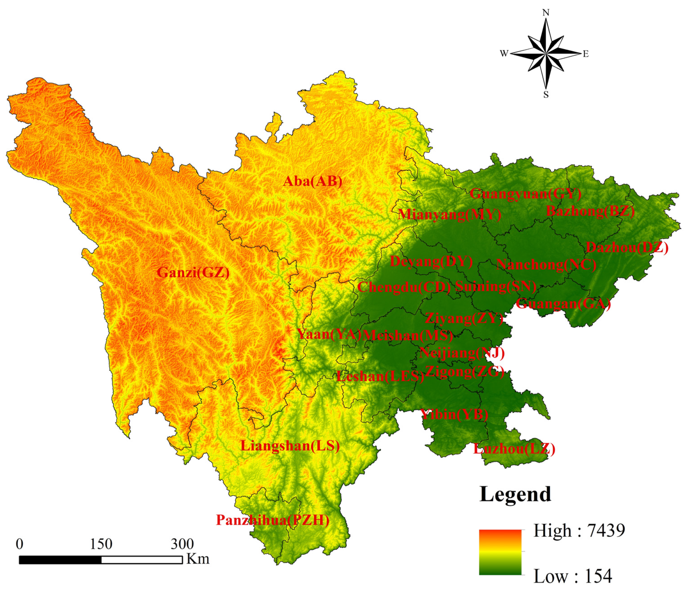
2.1. Overview of the Study Sites in Sichuan Province

Sichuan Province is located in the southwestern region of China, comprising 21 cities and prefectures including CD, MY and GZ Prefectures. The terrain in Sichuan Province significantly varies from east to west, with a complex and diverse landscape. GZ Prefecture, AB Prefecture, LS Prefecture and PZH City are at higher altitude and exhibit a plateau terrain, whereas CD, ZY and SN are plain basin regions (Figure 2).

Sichuan Province is a major agricultural production province in China that ranks sixth based on the size of arable land. The province is a national grain production base and of it is among the top three forest areas and top five pastoral areas in China. The agricultural production and development in this province exhibit a high degree of typicality and representativeness nationwide. However, Sichuan Province generates a high amount of carbon emissions during agricultural production, causing pollution to the environment. Therefore, Sichuan Province faces severe carbon reduction pressure during agricultural development. Although the total ACE in Sichuan Province gradually decreased from 2005 to 2020, with an average annual decrease of 0.62% [23], the total ACE are still high. Generation of ACE is linked to energy consumption, mainly comprising water energy, mechanical kinetic energy and petroleum products. In addition, energy consumption during manufacture of agricultural materials, such as agricultural films, fertilizers and pesticides, accounts for a high proportion of carbon emissions. Therefore, the authorities involved in agricultural development in Sichuan Province should advocate for reduced energy consumption and formulate policies to minimize carbon emissions.

2.2. Indicator Selection

This paper collected agricultural production data of 21 cities and prefectures in Sichuan Province from 2011 to 2020 (data are all from the Sichuan Statistical Yearbook) through a literature review to explore the current status of agricultural production in Sichuan Province from the perspective of WLEC. This paper constructed an input–output index system of APE related to WLEC based on findings from previous studies and the availability of data. The input indicators included the number of jobs related to agricultural activities, agricultural water consumption, the total area with planted crops, the total energy used by agricultural machinery and the amount of diesel oil used in agricultural activities. The expected output was the gross agricultural product. The unexpected output was the carbon emissions produced through agricultural activities. The reference basis of indicators used in this paper is shown in

Table 1. Criteria for indicator selection.

Categories	Specific Content	Unit	Indicator Code	Indicator Reference Source
Input indicators	Agricultural employment	Ten thousand	$X_1$	[24,25,26,27]
	Agricultural water	Million cubic meters	$X_2$
	Total planted area of crops	Kilograms	$X_3$
	Total power of machinery	Million kilowatts	$X_4$
	Amount of agricultural diesel	Tons	$X_5$
Expected output indicator	Gross agricultural product	Hundred million yuan	$Y_1$
Unexpected output indicator	Agricultural carbon emissions	kgCO2eq	$Y_2$

:

2.3. Introduction to Analytical Methods

This paper explored the factors that affect APE in Sichuan Province from the perspective of WLEC. An input–output index system associated with WLEC was constructed. The panel regression model was established to evaluate the factors that affect production efficiency based on the calculated APE. The methods used in determination of the effect of various factors on APE are presented as a flow chart in Figure 3:

2.3.1. Calculation of Carbon Dioxide Level

In the coupling relationship of WLEC, ACE are the most difficult indicator to calculate. At present, the main calculation methods for carbon emissions include the life cycle method, on-site exploration method and carbon emission factor method [28]. The carbon emission factor method was used in this paper and the formula is shown below:

$$c={\displaystyle \sum c_i}={\displaystyle \sum e_i\cdot {\epsilon }_i}$$

(1)

where c represents the total amount of ACE; $i$ denotes the type of carbon emission source; $e$ represents the amount of each carbon emission source; $\epsilon$ denotes the carbon emission coefficient corresponding to each carbon source.

The specific carbon source factor and its corresponding carbon emission coefficient are determined based on three aspects: (1) carbon dioxide emissions caused by agricultural materials, including agricultural chemical fertilizers, pesticides, agricultural film, four categories of diesel oils, all based on the actual use for the specific year; (2) the effective irrigation area required for agricultural production in the current year; (3) the nitrous oxide emission caused by tilling the land, which is dependent on the actual area with crops in the current year. Methane, carbon dioxide and nitrous oxide were uniformly converted into standard carbon equivalent according to the intensity of greenhouse effect for convenience of analysis [29].

2.3.2. Super-Efficient SBM Model

From the perspective of WLEC coupling, the calculation method of APE in Sichuan Province is the super-efficient SBM model [30], which is constructed as follows:

This paper assumed that there are n decision-making units, and each decision-making unit has three vectors, namely input, expected output and unexpected output. Subsequently, the paper used an input vector of q units to produce the expected output of $u_1$ units and unexpected output of $u_2$ units. The three vectors were $x\in R^q$, $y^g\in R^{u_1}$, $y^b\in R^{u_2}$, respectively. The matrix $X$, $Y^g$, $Y^b$ can be expressed as follows:

$$X=\left[x_1,\cdots ,x_n\right]\in R^{q\times n}>0$$

$$Y^g=\left[y_1^g,\cdots ,y_n^g\right]\in R^{u_1\times n}>0$$

$$Y^b=\left[y_1^b,\cdots ,y_n^b\right]\in R^{u_2\times n}>0$$

A production possibility set P containing the unexpected output can be constructed as follows: $P=\left\{\left(x,y^g,y^b\right)|x\ge X\lambda ,y^g\le Y^g\lambda ,y^b\ge Y^b\lambda ,\lambda \ge 0\right\}$.

According to the processing method of the super-efficient SBM model, the fractional programming form of the super-efficient SBM model considering the unexpected output is expressed as shown below:

$$AP{E}^{*}=\min \frac{\frac{1}{q}{\displaystyle \sum _{i=1}^q\frac{\overline{x_i}}{x_{i0}}}}{\frac{1}{u_1+u_2}({\displaystyle \sum _{r=1}^{u_1}\frac{{\overline{y}}_r^g}{y_{r0}^g}}+{\displaystyle \sum _{l=1}^{u_2}\frac{{\overline{y}}_l^b}{y_{l0}^b}})}$$

(2)

$$s.t\overline{x}\ge {\displaystyle \sum _{j=1,\ne 0}^n{\lambda }_j{x}_j}$$

$${\overline{y}}^g\le {\displaystyle \sum _{j=1,\ne 0}^n{\lambda }_j{y}_j^g}$$

$${\overline{y}}^b\ge {\displaystyle \sum _{j=1,\ne 0}^n{\lambda }_j{y}_j^b}$$

$$\overline{x}\ge x_0,{\overline{y}}^g\le y_0^g,{\overline{y}}^g\ge 0,\lambda \ge 0$$

In the above formula, $x$, $y^g$ and $y^b$ represent the input variables of the decision-making unit (agricultural employment, agricultural water consumption, total area with crops, total power utilized by machinery and agricultural diesel), expected output variables (gross agricultural production) and unexpected output variables (carbon dioxide emission). $s^{-}$, $s^g$, $s^b$ represent the relaxation vectors of the input variables, expected output and unexpected output, respectively, and $\lambda$ denotes the weight vectors. The subscript “0” in the model represents the evaluated unit. The value of the objective function $AP{E}^{*}$ is the $APE$ value. The $APE$ value can exceed 1 and it monotonically decreases with respect to $s^{-}$, $s^g$, $s^b$. The input–output ratio of $APE$ is the same when the values of $AP{E}^{*}\ge 1$, the values of $s^{-}$, $s^g$, $s^b$ are all 0. A value of $AP{E}^{*}<1$ indicates that $APE$ is at an unbalanced state, thus it is necessary to improve the input and output.

2.3.3. Malmquist Index

This article uses the relevant data of WLEC in Sichuan’s agricultural production from 2011 to 2020 to evaluate the APE of Sichuan Province over the past decade. In order to better study the spatiotemporal changes of APE in Sichuan Province from the perspective of WLEC coupling, this article adopts the Malmquist index model to analyze the temporal changes. The total factor productivity ($TFP$) can be decomposed into the technical efficiency change index ($EC$) and technical change index ($TC$) using the Malmquist productivity index method. In addition, $EC$ can be further decomposed into a pure technical efficiency change index ($PEC$) and scale efficiency change index ($SEC$) after it is converted from a scale to a variable. This Malmquist index can be used to evaluate the dynamic evolution and change in APE in Sichuan Province using dynamic data [31]. $TFP$ can be expressed as follows:

$$TFP=\frac{D^{t+1}(x_0^{t+1},y_0^{t+1})}{D^t(x_0^t,y_0^t)}{\left[\frac{D^t(x_0^{t+1},y_0^{t+1})}{D^{t+1}(x_0^{t+1},y_0^{t+1})}\times \frac{D^t(x_0^t,y_0^t)}{D^{t+1}(x_0^t,y_0^t)}\right]}^{\frac{1}{2}}$$

(3)

In Equation (3), $(x_0^t,y_0^t)$ represents the input at period $t$, $(x_0^{t+1},y_0^{t+1})$ represents the output at period $t+1$, $D^t$ and $D^{t+1}$ represents the distance functions at period $t$ and period $t+1$, respectively. A $TFP$ value greater than 1 indicates that the total factor production efficiency increases from period $t$ to period $t+1$, and a $TFP$ value less than 1 indicates that the total factor production efficiency decreases. The Malmquist index is decomposed as follows:

$$TFP=EC\times TC$$

(4)

$TC$ reflects the degree of impact due to the progress of production technology, which is exhibited by the possession of new knowledge or skills. A value of $TC>1$ indicates innovation or progress in technology, whereas a value of $TC$ less than 1 represents technological regression. $EC$ reflects the comprehensive utilization of existing technology. A value of $EC>1$ indicates an improvement in technical efficiency, while a value $EC$ less than 1 indicates a decrease in technical efficiency. Therefore, the Malmquist index can be used to effectively evaluate the degree of change in agricultural efficiency in Sichuan Province in different periods and can accurately reflect the differences in technological innovation and utilization.

2.3.4. Spatial Autocorrelation Analysis

In order to study the spatial differences in APE in Sichuan Province, this article uses spatial autocorrelation analysis. The spatial correlation of APE refers to whether the spatial distribution of APE is interrelated. Spatial autocorrelation analysis methods include global autocorrelation and local autocorrelation.

Using global spatial autocorrelation to analyze the APE in Sichuan Province can measure the degree of correlation between the APE of the entire Sichuan province and find out whether there is a significant spatial distribution pattern of APE in 21 cities and states. This paper used the global Moran I index to evaluate the spatial correlation of APE distribution in Sichuan Province. Further, this paper used the standardized $Z$ value to determine the significance level of the global Moran I index. The expressions for calculation of the global Moran I index and the $Z$ value [32] are presented below:

$$I=\frac{n{\displaystyle \sum _{i=1}^n{\displaystyle \sum _{j=1}^m{w}_{ij}(x_i-\overline{x})(x_j-\overline{x})}}}{{\displaystyle \sum _{i=1}^n{\displaystyle \sum _{j=1}^m{w}_{ij}{(x_i-\overline{x})}^2}}}$$

(5)

$$Z_{score}=\frac{I-E(I)}{\sqrt{Var(I)}}$$

(6)

In the formulas, $I$ represents the global Moran’s I index; $n$ denotes the total number of research subjects; $\overline{x}$ represents the average value of yield; $x_i$ and $x_j$ represents the APE of the $i$ and $j$ study areas, respectively. In the equation, $w_{ij}$ denotes the spatial weight coefficient of the $i$ and $j$ regions, which reflects the spatial relationship between regions $i$ and $j$ and is expressed as: whether the regions are adjacent, $w_{ij}=1$ or whether the regions are not adjacent $w_{ij}=0$. $E(I)$ and $Var(I)$ represent the expected value and variance of Moran’s I index, respectively. The range of the global Moran I index is $[-1,1]$; when $I$ is greater than 0 ($p<0.05$) this indicates a spatial positive correlation, implying that high (or low) yield values are significantly clustered in space; A value of $I$ equal to or close to 0 indicates that there is no spatial autocorrelation in adjacent areas, and the yield is randomly distributed; a value of $I$ less than 0 ($p<0.05$) indicates a negative spatial correlation, implying that the yield of adjacent regions is not correlated. $\left|Z_{score}\right|>1.96$ indicates a significant global Moran I index at a significance level of 0.05.

Compared to the global spatial autocorrelation analysis method used to study the overall distribution of APE in 21 cities and states in Sichuan Province, local spatial autocorrelation analysis focuses on the spatial correlation and heterogeneity of aggregation types, regions and surrounding neighborhoods in each city and state in Sichuan Province [33].

$$I=\frac{n(x_i-\overline{x})}{{\displaystyle \sum _{i=1}^n{(x_i-\overline{x})}^2}}{\displaystyle \sum _{i\ne j}^n{w}_{ij}(x_j-\overline{x})}$$

(7)

The coefficients in the equation represent the same variables described in Equation (5). The local spatial autocorrelation index ($I$) represents the spatial aggregation of various spatial units with similar heat values. A value of $I>0$ indicates that each unit exhibits an aggregated state in space. A value of $I<0$ indicates that each unit is in a discrete state in space [34,35].

2.3.5. Panel Regression Model

From the coupling perspective of WLEC, this article calculates the APE in Sichuan Province and analyzes the results in time and space. In order to better study the development characteristics of APE, this article explores its influencing factors. Statistical regression methods can be used to explore the degree of the effect of independent variables on dependent variables. Three types of regression analysis models are used in statistics and econometrics for analysis of panel data, namely the mixed estimation model, fixed effect model and random effect model [36,37]. This article uses a fixed effects model to analyze APE in Sichuan Province, and its mathematical expression is as follows:

$$AP{E}_{it}^{*}={\alpha }_i+X_{it}\alpha +{\epsilon }_{it}$$

(8)

In the above equation, $i=1,2,\dots ,N$ represents the number of influencing factors, $t=1,2,\dots ,T$ represents different years. $AP{E}_i^{*}$ denotes the dependent variable of APE. $X_{it}$ represents the influencing factor, ${\alpha }_i$ is a constant term, $\alpha$ represents the correlation coefficient vector, ${\epsilon }_{it}$ is independent error term and ${\epsilon }_{it}~N(0,{\sigma }^2)$.

3. Results

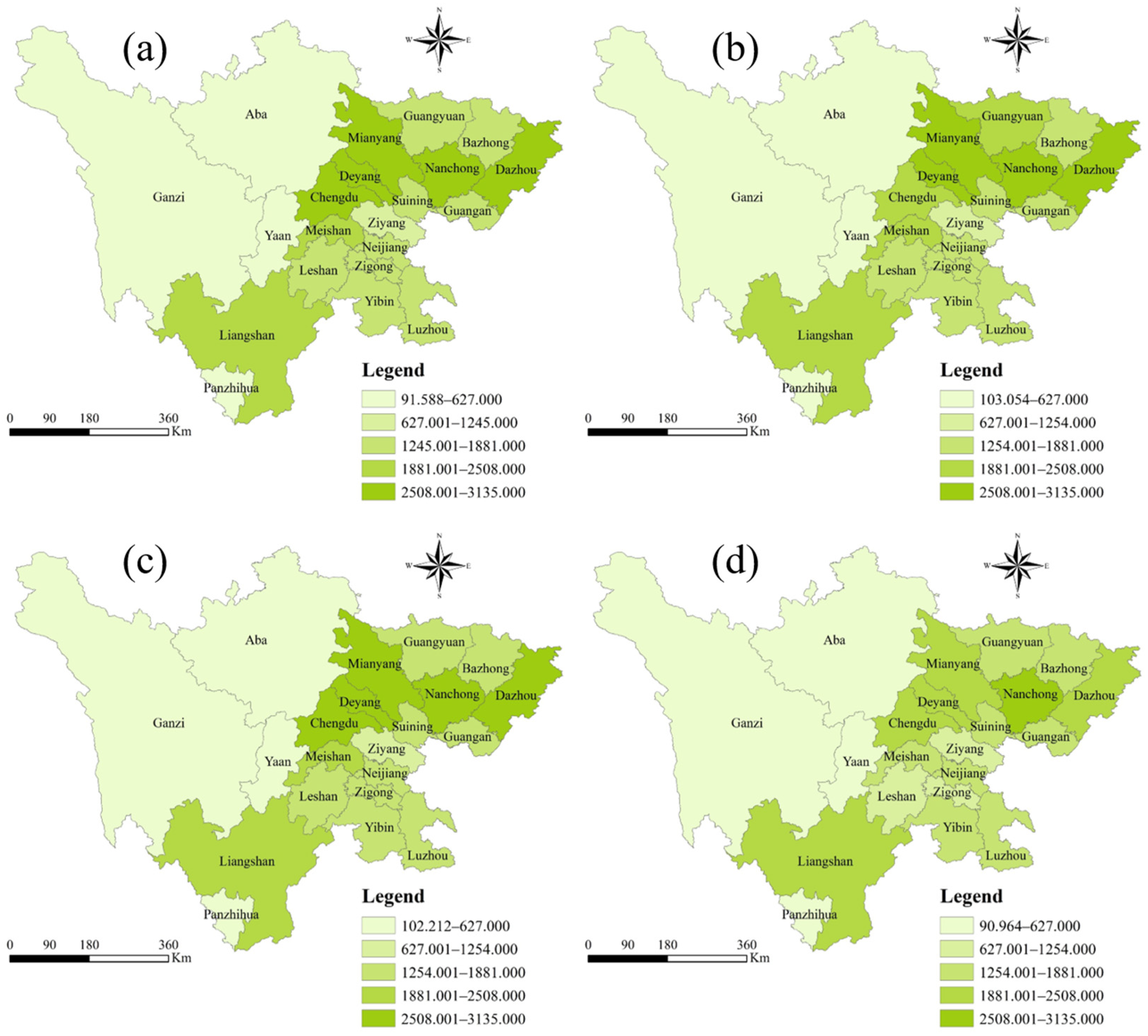
3.1. Calculation and Analysis of Agricultural Carbon Emissions

The results of ACE for the 21 cities and prefectures in Sichuan Province are shown in Figure 4. The results showed that: (1) The overall ACE in Sichuan Province were higher in the east and lower in the west. GZ Prefecture, AB Prefecture and YA City in the west of Sichuan Province had the lowest ACE compared with other regions in the province. ACE were generally higher in various cities and prefectures in the eastern Sichuan region. Cities in areas around the eastern part of the province such as MY, NC and DY exhibited the highest carbon emissions. (2) A subtle change was observed in the distribution of carbon emissions among various cities and prefectures in Sichuan Province from 2011 to 2020, but a significant difference was observed between the eastern and the western regions. The carbon emissions in NC reached 250.8 million kgCO₂eq in 2020, but the carbon emissions in the northeast region of Sichuan generally decreased compared with other years.

3.2. Temporal and Spatial Analysis of Agricultural Production Efficiency in Sichuan Province

From the perspective of WLEC coupling, analyzing the spatiotemporal characteristics of APE in Sichuan Province requires a reasonable calculation of APE. The number of people employed in the agricultural sector, agricultural water consumption, total planting area, total mechanical power and agricultural diesel were utilized as input indicators for determination of APE using the super-efficient SBM model. The gross agricultural product represented the expected output indicators and the carbon emission level related to agricultural production activities represented the non-expected output. A super-efficient SBM model was constructed using these indicators to evaluate the APE of 21 cities and prefectures in Sichuan Province from 2011 to 2020.

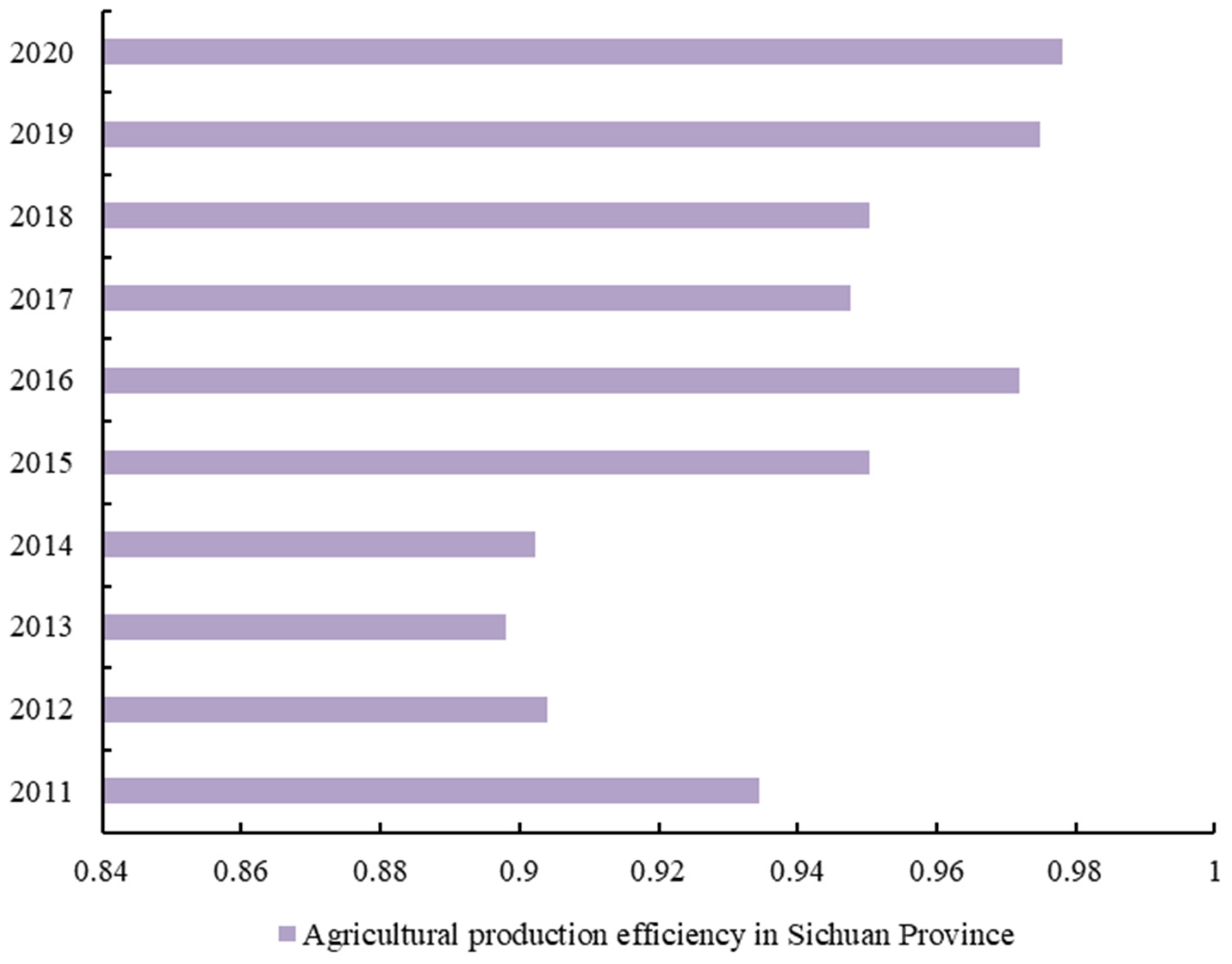
3.2.1. Analysis of Temporal Changes in Agricultural Efficiency in Sichuan Province

This paper used the MAXDEA 6 software to calculate the APE values of Sichuan Province from 2011 to 2020 (Figure 5). The results show that: (1) The entire Sichuan Province had a high APE above 0.88 from 2011 to 2020, indicating a high level of agricultural development (Figure 5). These findings show a high level of utilization of water resources, land resources and energy in the agricultural production process and relatively low level of carbon emissions in Sichuan Province. (2) The APE in Sichuan Province fluctuates significantly in various years, with a fluctuating and increasing trend. The APE in Sichuan Province was approximately 0.94 in 2011. A decrease in APE was observed from 2012 to 2014, and this period exhibited the lowest efficiency throughout the study period. The APE increased from 2015 to 2016, then a slight decrease was observed from 2017 to 2018. APE increased from 2019 to 2020, reaching the highest level.

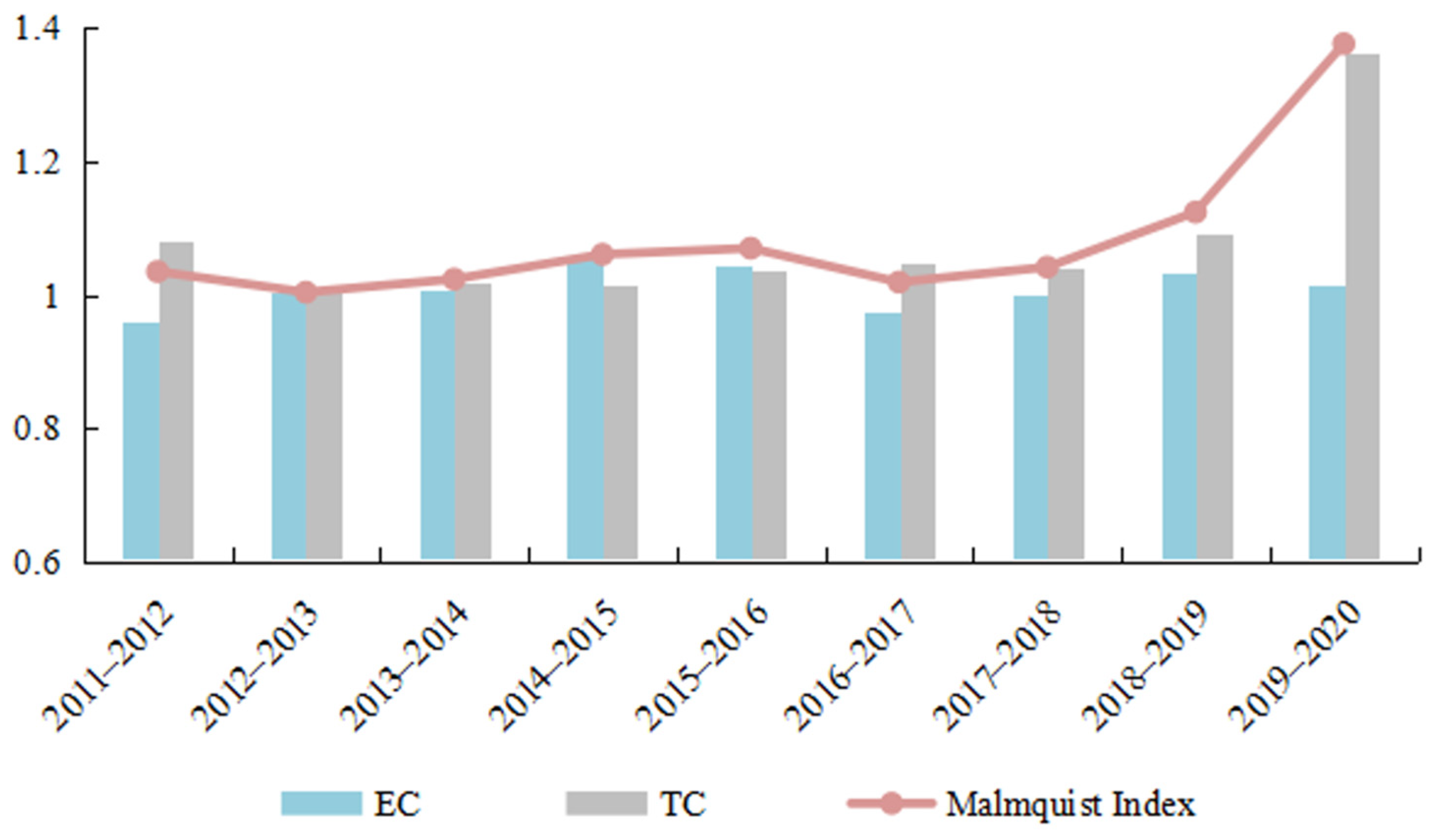
3.2.2. Malmquist Index Analysis of Agricultural Production Efficiency in Sichuan Province

This article calculated the dynamic changes in the Malmquist index of APE in Sichuan Province, as well as the corresponding EC and TC to further explore the annual changes in APE and determine whether the changes were due to improved efficiency or enhanced APE caused by technological progress (Figure 6).

The results showed that: (1) The Malmquist index of cities in Sichuan Province was greater than 1 (Figure 6). Notably, the Malmquist index fluctuated and increased over the years. The overall APE in Sichuan Province increased with time. The Malmquist index significantly increased from 2018 to 2020, reaching its peak in 2020, with a peak value of about 1.4. The efficiency of agricultural production in 2020 exhibited an approximately 40% increase compared with 2019. (2) Analysis of the EC and TC showed a subtle difference in changes between the TC and the Malmquist index. The increase in APE was mainly attributed to TC. A TC greater than 1 indicates continuous technological progress. (3) The EC was less than 1 in 2011–2012 and 2016–2018, indicating a decline in EC in 2012, 2017 and 2018, and the need for improving the EC.

3.2.3. The Global Moran Index of Agricultural Production Efficiency in Sichuan Province

Analysis of APE in Sichuan Province based on WLEC coupling should be conducted from the perspective of time and the perspective of spatial correlation to explore the changes in agricultural production caused by different geographical locations in Sichuan Province. This paper selected 2011, 2014, 2017 and 2020 for analysis to further explore the global spatial autocorrelation. Moran’s I index showed that the spatial correlation of agricultural production in Sichuan Province was relatively weak (

Table 2. Moran’s I index of Sichuan Province in 2011, 2014, 2017 and 2020.

Time	2011	2014	2017	2020
Moran’s I	0.0035	−0.0263	0.0234	−0.0527

). The results indicated that the high and low distribution of APE in Sichuan Province was random and not completely clustered or dispersed in the region. Therefore, it is imperative to enhance the collaborative capacity and level of agricultural production in Sichuan Province.

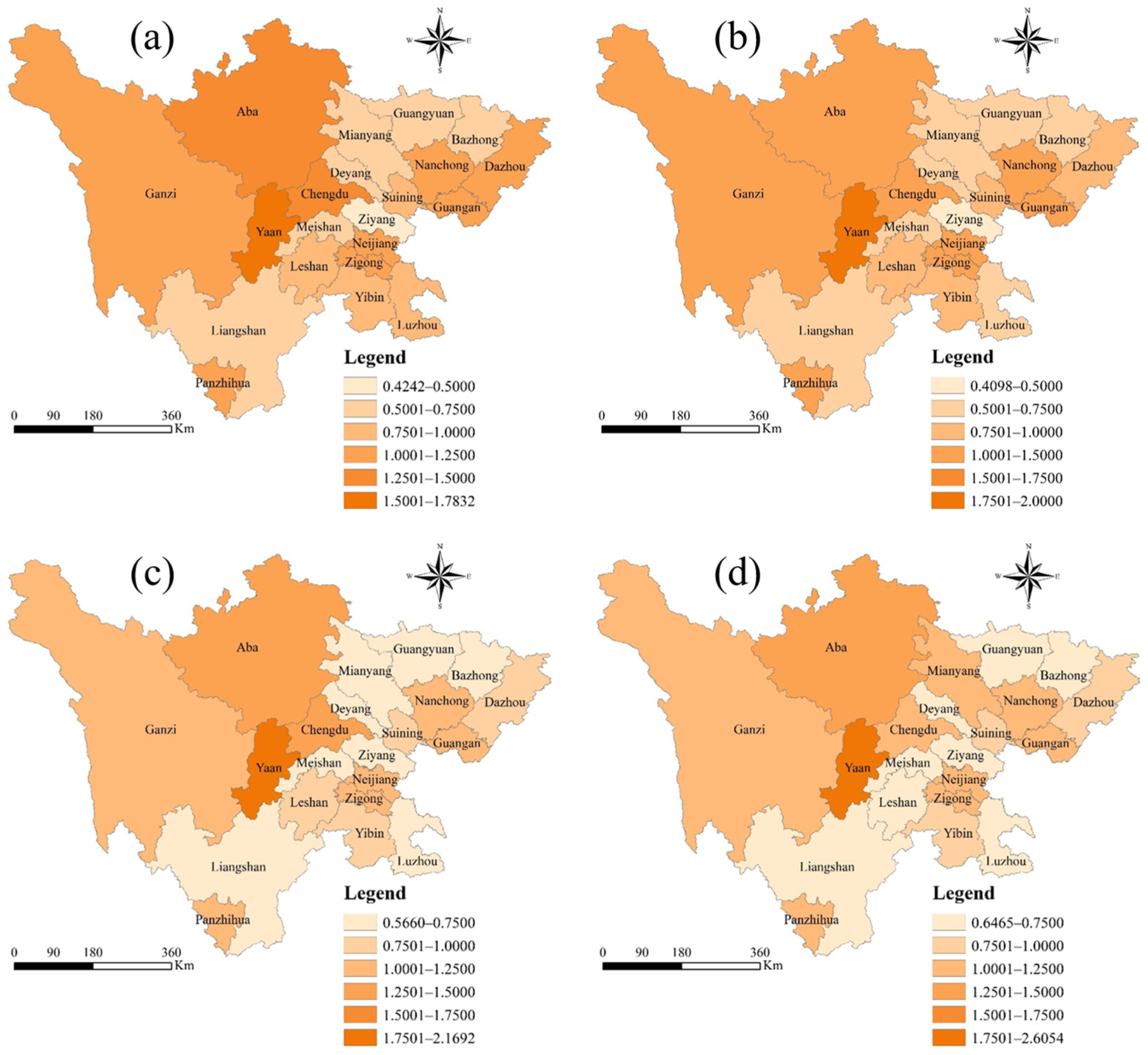
3.3. Spatiotemporal Analysis of Agricultural Production Efficiency in 21 Cities and Prefectures in Sichuan

From the perspective of WLEC coupling, the spatiotemporal characteristics of overall APE in Sichuan Province were analyzed. In order to more accurately study the changes in APE in Sichuan and the development of agricultural production in various cities and states, it is necessary to conduct temporal and spatial research on the APE of 21 cities and states in Sichuan Province.

3.3.1. Analysis of Temporal Changes in Agricultural Efficiency in Various Cities and Prefectures

In this paper, the MAXDEA 6 software was used to calculate the APE values of 21 cities and prefectures in Sichuan Province from 2011 to 2020. Representative results are shown in Figure 7. The results showed: (1) Under the coupling perspective of WLEC, there is a significant difference in APE among 21 cities and prefectures in Sichuan Province. YA had the highest APE, followed by CD, GZ, AB and PZH. The APE in BZ, DY, ZY, GY, LS prefectures and other places was relatively low throughout the study period. The APE in western Sichuan was higher and lower in northeastern Sichuan, which is an opposite trend to the level of ACE. Carbon emissions, which were the unexpected output in this paper, negatively affect APE. (2) The changes in APE of various cities and prefectures in Sichuan Province were not significant from 2011 to 2020. However, a significant increase in APE was observed in 2020, with more than 0.6465 APE of all cities and prefectures in Sichuan Province. The APE of some cities, such as ZY, greatly improved over time. In addition, the APE of YA, AB prefectures, and CD significantly improved over the study period.

Further analysis was conducted to determine the level of APE in the entire Sichuan Province and the changes over time and space. The APE of 21 cities and prefectures in Sichuan Province from 2011 to 2020 is presented in

Table 3. Agricultural production efficiency of 21 cities and prefectures in Sichuan Province from 2011 to 2020.

Cities	2011	2012	2013	2014	2015	2016	2017	2018	2019	2020	Mean
CD	1.348	1.358	1.378	1.414	1.562	1.449	1.437	1.451	1.373	1.073	1.384
ZG	1.144	1.146	1.079	1.046	1.052	1.131	1.085	1.075	1.085	1.138	1.098
PZH	1.201	1.136	1.147	1.198	1.116	1.160	1.088	1.069	1.073	1.076	1.126
LZ	0.853	0.801	0.803	0.722	0.705	0.760	0.702	0.711	0.727	0.740	0.752
DY	0.621	0.629	0.665	0.648	0.643	0.704	0.682	0.662	0.676	0.723	0.665
MY	0.642	0.628	0.642	0.634	0.674	0.716	0.687	0.679	0.728	1.013	0.704
GY	0.587	0.517	0.530	0.531	0.576	0.611	0.585	0.586	0.610	0.647	0.578
SN	0.789	0.730	0.760	0.790	0.758	1.008	0.829	0.798	0.896	0.908	0.827
NJ	1.053	1.007	0.791	1.016	1.049	1.071	1.078	1.058	1.071	1.017	1.021
LES	0.771	0.770	0.816	0.832	0.854	0.878	0.841	0.860	0.822	0.720	0.816
NC	1.149	1.247	1.258	1.244	1.199	1.193	1.190	1.173	1.145	1.046	1.184
MS	0.552	0.596	0.606	0.610	0.645	0.639	0.692	0.693	0.698	0.661	0.639
YB	0.829	0.751	0.758	0.766	1.001	1.027	0.794	0.801	0.806	0.861	0.839
GA	1.168	1.157	1.198	1.097	1.076	1.047	1.057	1.097	1.055	1.052	1.100
DZ	1.071	0.872	0.851	0.863	0.891	0.884	0.877	0.873	1.002	0.904	0.909
YA	1.783	1.792	1.769	1.784	1.851	2.137	2.169	2.305	2.456	2.605	2.065
BZ	0.581	0.494	0.499	0.515	0.550	0.557	0.566	0.566	0.632	0.723	0.568
ZY	0.424	0.389	0.415	0.410	0.411	0.546	0.575	0.565	0.643	0.668	0.505
AB	1.307	1.329	1.193	1.179	1.265	1.202	1.282	1.244	1.265	1.255	1.252
GZ	1.043	1.013	1.014	1.002	1.433	1.000	1.024	1.028	1.018	1.013	1.059
LS	0.710	0.619	0.686	0.647	0.648	0.688	0.659	0.663	0.688	0.697	0.671

.

Table 3 shows that (1) the APE values of ZY, BZ, GY, MS, DY, LS prefectures, LZ and LES from 2011 to 2020 were less than 1, indicating that the APE was at a low level during these 10 years. This implies that various strategies can be used to improve the APE. The integration of resources and environmental management have not significantly improved APE. These cities have relatively lower level of APE in Sichuan Province compared with other cities. (2) The average APE of cities such as GZ prefecture, ZG, GA, PZH, NC, AB prefectures, CD and YA was 1 during the study period, and the annual APE was greater than 1. The APE of these cities and prefectures is markedly high, owing to effective control of ACE and WLE distribution during agricultural production. (3) The APE of various cities and prefectures in Sichuan Province exhibits insignificant fluctuation throughout the study period, with all values close to the mean value. This indicates that the agricultural production level of various cities and prefectures in Sichuan Province did not improve or decrease significantly from 2011 to 2020. Agricultural production level is a gradual process and cannot rapidly reach a higher level. Therefore, strategies should be explored that improve the agricultural development efficiency within a short time and improve the quality of agricultural development.

3.3.2. Malmquist Index Analysis of Agricultural Production Efficiency in Various Cities and Prefectures of Sichuan

We further analyzed the temporal changes in APE of 21 cities and states in Sichuan Province, and calculated the Malmquist index results of APE of 21 cities and states, as shown in

Table 4. Malmquist index and mean of each city and prefecture in Sichuan Province.

Cities	2011–2012	2012–2013	2013–2014	2014–2015	2015–2016	2016–2017	2017–2018	2018–2019	2019–2020	Mean
CD	1.113	1.003	1.039	1.160	1.002	1.030	1.057	1.136	0.993	1.059
ZG	1.422	0.627	0.993	0.995	1.189	0.967	1.008	1.105	1.399	1.078
PZH	0.942	1.092	1.088	1.063	1.093	0.984	0.990	1.168	1.189	1.068
LZ	0.954	1.011	0.981	0.960	1.110	0.927	1.045	1.136	1.308	1.048
DY	1.085	1.041	1.030	1.080	1.111	1.013	1.031	1.093	1.139	1.069
MY	1.066	0.996	0.993	1.124	1.060	0.996	1.044	1.138	1.434	1.095
GY	1.007	1.012	1.018	1.089	1.077	0.994	1.034	1.098	1.317	1.072
SN	1.038	1.020	1.071	0.977	1.154	0.968	1.016	1.172	1.197	1.068
NJ	0.929	0.992	1.136	1.033	1.105	1.016	0.950	1.083	1.463	1.079
LES	1.065	1.033	1.067	1.064	1.030	0.998	1.050	1.048	1.159	1.057
NC	1.127	0.968	1.014	1.014	1.028	1.008	1.026	1.065	1.205	1.051
MS	1.126	1.008	1.087	1.070	1.085	1.079	1.039	1.086	1.178	1.084
YB	0.956	0.998	1.017	1.098	1.074	0.950	1.049	1.105	1.339	1.065
GA	0.986	1.143	0.874	1.060	1.012	1.027	1.303	1.037	1.387	1.092
DZ	0.984	0.954	1.019	1.042	1.037	1.001	1.016	1.117	1.189	1.040
YA	1.081	1.051	1.051	1.088	1.014	1.088	1.071	1.152	2.731	1.259
BZ	0.960	0.983	1.027	1.054	1.022	1.035	1.034	1.186	1.430	1.081
ZY	1.008	1.050	0.993	1.011	1.276	1.114	1.007	1.255	1.281	1.111
AB	0.966	0.926	1.041	1.143	0.933	1.130	1.005	1.127	1.599	1.097
GZ	0.966	1.099	0.974	1.082	0.987	1.086	1.036	1.159	1.731	1.124
LS	0.949	1.070	0.978	1.062	1.067	0.988	1.057	1.135	1.236	1.060

:

Table 4 shows that: (1) The Malmquist index of APE in 21 cities and states in Sichuan Province was greater than 1, indicating that the APE of each city and state in Sichuan Province has increased over time, but the magnitude of the improvement varies each year. The results show that the Malmquist index in DZ City was the lowest at 1.040, whereas the Malmquist index in YA City was 1.259. The APE and Malmquist index were the highest in the province. The overall agricultural production level in YA City was relatively high, and agricultural development has been increasing every year, which is higher than the agricultural development level of other cities. (2) The annual Malmquist indexes of DY, GY, MS and YA were greater than 1, indicating that the agricultural productivity of these cities has been increasing every year, and the technological level of agricultural production is constantly improving. The allocation of agricultural production resources and environmental management were also relatively high. (3) The Malmquist index of each city and state fluctuated around 1 from 2011 to 2020, without exhibiting significant increase or decrease. Similar observation was made for the APE values of each city and state, implying that agricultural development will not reach a new level soon but requires a gradual development process. However, the efficiency of agricultural production in all cities except PZH, NJ and CD has continuously improved in the last three years, indicating that these three cities have experienced a decline in agricultural development compared with the other three cities and should formulate strategies to reduce carbon emissions.

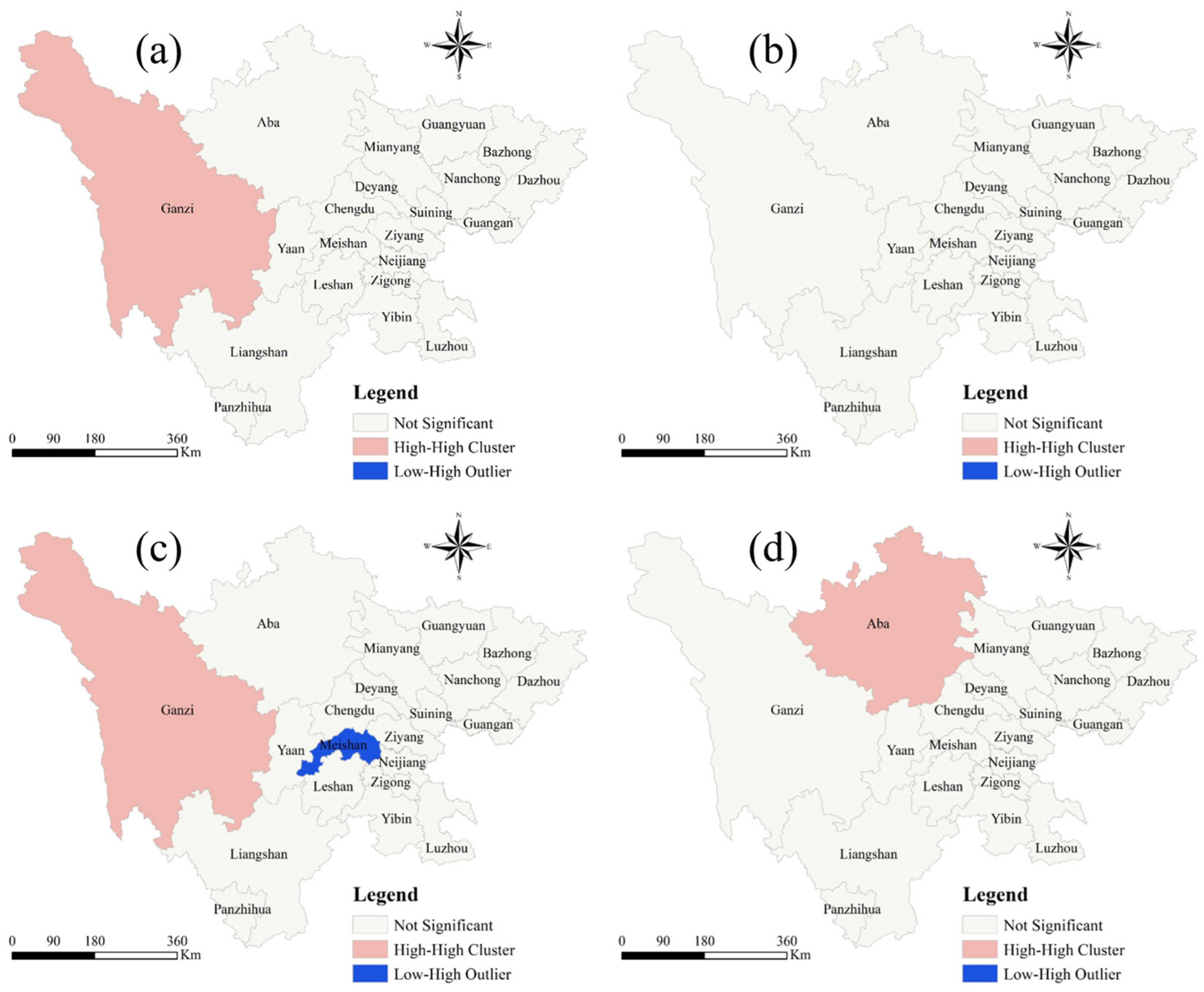
3.3.3. Local Spatial Autocorrelation of Agricultural Production Efficiency in Various Cities and Prefectures of Sichuan

After conducting a global spatial autocorrelation analysis of Sichuan Province, it can be found that the overall distribution of APE in Sichuan Province is random. When analyzing various cities and states, local spatial autocorrelation can be used to examine the correlation between APE in a small number of regions. Similar to the global spatial autocorrelation in Sichuan Province, data from 2011, 2014, 2017 and 2020 were selected for local spatial autocorrelation analysis. The results are shown in Figure 8:

The results showed that: (1) In 2011, a high clustering center was formed with GZ prefecture as the center (Figure 8). The APE in the cities and prefectures surrounding the GZ prefecture, AB prefecture, YA City and LS prefecture was also high. However, the APE in other regions did not exhibit a clustering effect. (2) The APE of all cities and prefectures in Sichuan Province did not show a high or low clustering effect in 2014. The distribution of APE in the entire province was relatively random in 2014. (3) Two clusters were observed in 2017. The first was the high cluster centered around GZ prefecture. The APE of AB prefecture, YA City and LS prefecture was significantly high. On the contrary, the APE of MS was not high, but the APE of YA, LS, CD, NJ and ZG around MS was relatively high. (4) A high cluster was observed around AB prefecture in 2020. The APE of CD, MY, GZ prefectures and YA was relatively high. The spatial correlation of the APE of the whole Sichuan Province showed that the APE was high in AB prefecture, GZ prefecture and YA City. The distribution of APE in other regions was relatively random.

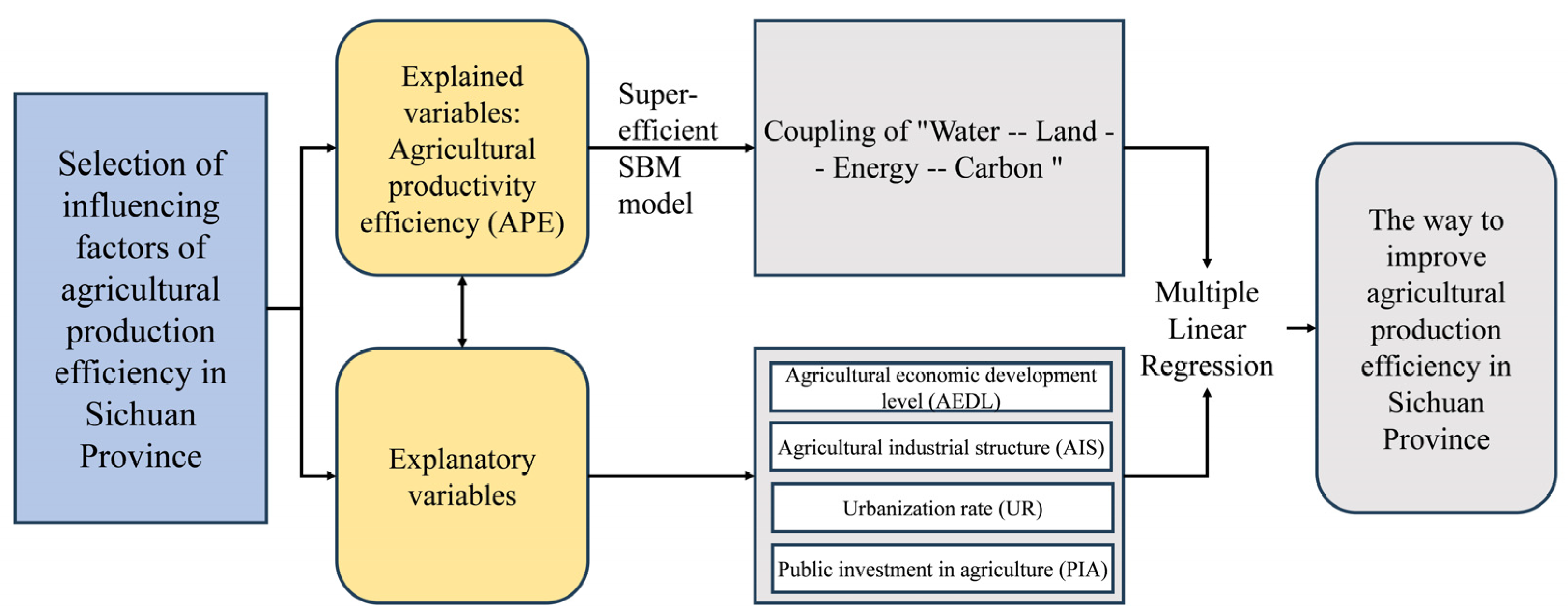
3.4. Factors Influencing Agricultural Production Efficiency in Sichuan Province

This paper explored and analyzed the spatiotemporal efficiency of agricultural production in Sichuan Province from the coupling perspective of WLEC. This paper used panel regression analysis to evaluate the factors that affect APE in Sichuan Province to provide information on improving APE and design strategies to improve APE in this province.

Literature review showed that APE is associated with various factors such as urbanization, the level of agricultural economic development and the industrial structure of agriculture [20,21,22]. Therefore, this paper established an explanatory variable and dependent variable based on panel regression model. The specific analysis framework and variable selection are shown in Figure 9.

APE is the agricultural production efficiency calculated using the super-efficient SBM model. AEDL is the ratio of the gross agricultural product to the total rural population. This ratio is used to evaluate the impact of agricultural development on people’s lives. AIS is the ratio of the total output value of agricultural production to the total output value of the primary industry and is used to determine the proportion of agricultural production. UR is the ratio of urban population to total population, which indicates the level of economic development of a region. PIA is the ratio of the government’s investment in agriculture to the total government investment in all sectors, which reflects the amount of government investment in agriculture.

This present study analyzed the super-efficient SBM model of various cities and prefectures in Sichuan Province from 2011 to 2020 from the perspective of WLEC. This paper used panel regression to explore the factors that affect APE. The panel regression model established in the paper is presented below:

$$AP{E}_t^{*}={\alpha }_0+{\alpha }_{1}U{R}_t+{\alpha }_{2}ADE{L}_t+{\alpha }_{3}PI{A}_t+{\alpha }_{4}AI{S}_t+{\epsilon }_t$$

(9)

where t = 2011, …, 2020, α₀ is a constant and α₁, α₂, α₃, α₄ represent the estimated parameters of the explanatory variable. ε_t denotes the error term. Multicollinearity was eliminated and the solution results were as follows:

The results showed that: (1) PIA and AIS were not correlated with APE, but UR, AEDL and C were significantly correlated with APE (

Table 5. Factors that modulate agricultural production efficiency.

Explanatory Variables	Regression Coefficient	Standard Error	t	p
C	1.164 ***	0.192	6.06	0.000
UR	−0.988 **	0.473	−2.09	0.038
PIA	−0.279	0.252	−1.11	0.269
AEDL	0.261 ***	0.062	4.18	0.000
AIS	−0.330	0.447	−0.74	0.461

** and *** represent 5% and 1% significance levels, respectively.

). (2) UR was negatively correlated with the efficiency of agricultural production, with a correlation coefficient of −0.988. This finding indicates that, for every unit increase in UR, the efficiency of agricultural production decreases by 0.988 units. (3) AEDL was significantly positively correlated with APE, with a correlation coefficient of 0.261. This result indicates that APE increases by 0.261 units as AEDL increases by 1 unit.

4. Conclusions

Improving APE and ensuring sustainable agricultural development are important issues in most developing countries, thus several scholars have explored this field. This paper explored the spatiotemporal characteristics of APE in Sichuan Province from the coupling perspective of WLEC, evaluated the influencing factors and further explored novel strategies for improving APE in Sichuan Province.

The results showed that: (1) The ACE in Sichuan Province exhibited a spatial pattern between 2011 and 2020, with higher levels in the east and lower levels in the west, mainly due to the different landforms in Sichuan Province resulting in significant regional differences. (2) The spatiotemporal characteristics of APE in Sichuan Province were evaluated from the perspective of WLEC coupling and the findings showed that: (I) The overall agricultural production level in Sichuan Province was relatively high, with a value of APE above 0.88. However, significant differences were observed between regions, which is not consistent with the profile of ACE. Therefore, appropriate agricultural development methods should be selected based on the natural environment of different regions in Sichuan Province to improve agricultural productivity. (II) The overall Malmquist index of Sichuan Province and the Malmquist index of various cities and prefectures were above 1 from 2011 to 2020. The levels of agricultural productivity gradually increased over time and the improvement in APE was mainly attributed to technological progress. Therefore, agricultural production in Sichuan Province can be improved by enhancing technological innovation and establishment of a green agricultural production technology system. The spatial clustering effect of APE was not very prominent. The level of APE in most cities was randomly distributed, and the correlation between the regions was weak. Therefore, the spatial allocation of resources for agricultural production in Sichuan Province should be optimized to establish a clustering effect and ensure agricultural development and progress. (3) Analysis of the influencing factors of APE showed that UR was negatively correlated with APE, whereas AEDL was positively correlated with APE. The differences in the effect of the different influencing factors can be explained as follows: (I) The labor cost of farming has increased due to urbanization, farming land and agricultural activities have been abandoned and the extensive use of agricultural machinery and equipment has increased the level of carbon emissions. (II) Income from agricultural activities can increase if the agricultural economy improves and the enthusiasm of farmers for agricultural production also increases. In addition, an improved agricultural economy can enhance investment in technological innovation, lead to use of efficient and low-carbon tools and promote the increase in APE. The results on the influencing factors indicate that stakeholders in agricultural production in Sichuan Province should actively advocate for an improvement of the relationship between agricultural production and urbanization, enhance agricultural economic development and increase investment in agricultural technology innovation.

The research results provide a systematic reference for future research in this field, and information for improving APE and sustainable development in Sichuan Province. These findings also provide necessary information for formulation of policies for the practical promotion of low-carbon agricultural production in Sichuan Province, and have significant implications for improving agricultural production while ensuring carbon reduction in Sichuan Province.

5. Discussion

The comprehensive analysis of agricultural development based on the WLEC coupling perspective has become an important research topic, and several scholars have explored agricultural production from multiple perspectives around the WLEC relationship. For example, the framework of regional agricultural greenhouse gas emissions was used to evaluate the relationship between the interaction of WLE and the factors that affect agricultural greenhouse gas emissions [38]. In addition, a multi-objective optimization model that utilizes a WLEC coupling system was developed to optimize the allocation of water and land resources in agricultural production processes [39]. In the context of “double carbon”, this paper is based on the WLEC coupling perspective. Therefore, this paper constructed an APE analysis model, evaluated the spatiotemporal characteristics of APE in Sichuan Province and used regression models to evaluate the factors that affect APE and explored targeted strategies to improve APE. This paper provides new ideas and methods for evaluation of APE in Sichuan Province. In addition, it provides a reference and basis for formulation of policies for improving low-carbon agricultural production in Sichuan Province. The paper has certain reference significance for achieving the regional “double carbon” goal.

The paper had some limitations and further studies can be conducted to improve the reliability of the findings. This paper did not consider the specific changes between WLEC, but only calculated the APE values of Sichuan Province as a whole and the values for each city and state, without a comprehensive analysis of the specific allocation of resources. Few factors affecting APE were selected in this paper due to limited availability of data, and factors such as the cultural quality of agricultural producers and the amount of imported agricultural products from rural areas were not included in the paper, thus more diverse factors should be explored in future studies [40]. Moreover, there are significant differences in the natural geography of Sichuan Province, and distinct studies have not been conducted on the geographical characteristics of various regions in Sichuan Province. Different regional differences were not considered during analysis of the influencing factors for each region [41].

Therefore, studies should be conducted to explore the overall relationship between WLEC and determine the changes in various indicators of WLEC and explore the level each indicator should be improved or reduced to achieve optimal efficiency. In addition to the four factors evaluated in this paper, factors such as the cultural level of workers, foreign imports and natural disasters should be explored to provide more detailed strategies for improving agricultural production and ecological construction, and ensuring sustainable production in Sichuan Province, to help mitigate global climate change. Moreover, research can be conducted based on the natural environment and other conditions in the different geographical regions to achieve effective development of agricultural production tailored to the local conditions.

References

1. Mi, Z.; Meng, J.; Guan, D.; Song, M.; Wei, Y.; Liu, Z.; Hubacek, K. Chinese CO2 emission flows have reversed since the global financial crisis. Nat. Commun. 2017, 8, 1712. [Google Scholar] [CrossRef] [PubMed]
2. Huang, X.; Xu, X.; Wang, Q.; Zhang, L.; Gao, X.; Chen, L. Assessment of agricultural carbon emissions and their spatiotemporal changes in China, 1997–2016. Int. J. Environ. Res. Public Health 2019, 16, 3105. [Google Scholar] [CrossRef] [PubMed]
3. Paustian, K.; Cole, C.V.; Sauerbeck, D.; Sampson, N. CO2 mitigation by agriculture: An overview. Clim. Chang. 1998, 40, 135–162. [Google Scholar] [CrossRef]
4. Johnson, M.F.; Franzluebbers, A.J.; Weyers, S.L.; Reicosky, D.C. Agricultural opportunities to mitigate greenhouse gas emissions. Environ. Pollut. 2007, 150, 107–124. [Google Scholar] [CrossRef] [PubMed]
5. Wei, T.; Dan, X. Examination and Analysis of Kuznets Curve of Chinese Agricultural Environment—Based on the Perspective of Carbon Emission. Ecol. Econ. 2017, 33, 37–40. [Google Scholar]
6. Vleeshouwers, L.M.; Verhagen, A. Carbon emission and sequestration by agricultural land use: A model study for Europe. Glob. Chang. Biol. 2010, 8, 519–530. [Google Scholar] [CrossRef]
7. Michael, M.; Dominic, M.; Vera, E.; Rees, R.M.; Andrew, B.; Cairistiona, F.E.T.; Bruce, B.; Steve, H.; Eileen, W.; Alistair, M.; et al. Developing greenhouse gas marginal abatement cost curves for agricultural emissions from crops and soils in the UK. Agric. Syst. 2010, 103, 198–209. [Google Scholar]
8. Ringler, C.; Bhaduri, A.; Lawford, R. The nexus across water, energy, land and food (WELF): Potential for improved resource use efficiency? Curr. Opin. Environ. Sustain. 2013, 5, 617–624. [Google Scholar] [CrossRef]
9. Silalertruksa, T.; Gheewala, S.H. Land-water-energy nexus of sugarcane production in Thailand. J. Clean. Prod. 2018, 182, 521–528. [Google Scholar] [CrossRef]
10. Bukhary, S.; Batista, J.; Ahmad, S. Water-energy-carbon nexus approach for sustainable large-scale drinking water treatment operation. J. Hydrol. 2020, 587, 124953. [Google Scholar] [CrossRef]
11. Wu, H.; Yang, T.; Liu, X.; Li, H.; Gao, L.; Yang, J.; Li, X.; Zhang, L.; Jiang, S. Towards an integrated nutrient management in crop species to improve nitrogen and phosphorus use efficiencies of Chaohu Watershed. J. Clean. Prod. 2020, 272, 122765. [Google Scholar] [CrossRef]
12. Tian, H.; Lu, C.; Pan, S.; Yang, J.; Miao, R.; Ren, W.; Yu, Q.; Fu, B.; Jin, F.-F.; Lu, Y.; et al. Optimizing resource use efficiencies in the food–energy–water nexus for sustainable agriculture: From conceptual model to decision support system. Curr. Opin. Environ. Sustain. 2018, 33, 104–113. [Google Scholar] [CrossRef]
13. Xu, Z.; Chen, X.; Liu, J.; Zhang, Y.; Chau, S.; Bhattarai, N.; Wang, Y.; Li, Y.; Connor, T.; Li, Y. Impacts of irrigated agriculture on food-energy-water-CO2 nexus across metacoupled systems. Nat. Commun. 2020, 11, 5837. [Google Scholar] [CrossRef] [PubMed]
14. Li, H.; Zhao, Y.; Lin, J. A review of the energy–carbon–water nexus: Concepts, research focuses, mechanisms, and methodologies. Wiley Interdiscip. Rev. Energy Environ. 2019, 9, e358. [Google Scholar] [CrossRef]
15. Meng, F.; Liu, G.; Liang, S.; Su, M.; Yang, Z. Critical review of the energy-water-carbon nexus in cities. Energy 2019, 171, 1017–1032. [Google Scholar] [CrossRef]
16. Albrecht, T.R.; Crootof, A.; Scott, C.A. The water-energy-food nexus: A systematic review of methods for nexus assessment. Environ. Res. Lett. 2018, 13, 043002. [Google Scholar] [CrossRef]
17. El Gafy, I.; Grigg, N.; Reagan, W. Water-food-energy nexus index to maximize the economic water and energy productivity in an optimal cropping pattern. Water Int. 2017, 42, 495–503. [Google Scholar] [CrossRef]
18. Smidt, S.J.; Haacker, E.M.; Kendall, A.D.; Deines, J.M.; Pei, L.; Cotterman, K.A.; Li, H.; Liu, X.; Basso, B.; Hyndman, D.W. Complex water management in modern agriculture: Trends in the water-energy-food nexus over the High Plains Aquifer. Sci. Total Environ. 2016, 566–567, 988–1001. [Google Scholar] [CrossRef] [PubMed]
19. Zhao, R.; Liu, Y.; Tian, M.; Ding, M.; Cao, L.; Zhang, Z.; Chuai, X.; Xiao, L.; Yao, L. Impacts of water and land resources exploitation on agricultural carbon emissions: The water-land-energy-carbon nexus. Land Use Policy 2018, 72, 480–492. [Google Scholar] [CrossRef]
20. Zhou, P.; Yang, S.; Wu, X.; Shen, Y. Calculation of regional agricultural production efficiency and empirical analysis of its influencing factors-based on DEA-CCR model and Tobit model. J. Comput. Methods Sci. Eng. 2022, 22, 109–122. [Google Scholar] [CrossRef]
21. Wang, J.; Li, J.; Zhou, C.; Zhou, S. Studies on Agricultural Production Efficiency around Dongting Lake in Hunan Province Based on DEA-Tobit Model. Tianjin Agric. Sci. 2019, 12, 48–55. [Google Scholar]
22. Huang, J.; Chen, M.; Liu, C. Has the development of agricultural production cooperation organization improved the efficiency of agricultural production—Analysis of provincial panel data based on Yangtze River Economic Belt. J. Shandong Agric. Univ. (Soc. Sci. Ed.) 2019, 2, 52–59+157. [Google Scholar]
23. Lu, Y.; Tian, Y.; Zhou, L. Spatial-Temporal Evolution and Influencing Factors of Agricultural Carbon Emissions in Sichuan Province. Agric. Resour. Reg. China 2021. Available online: https://kns.cnki.net/KCMS/detail/detail.aspx?dbcode=CAPJ&filename=ZGNZ2023011600D&dbname=CAPJLAST (accessed on 25 September 2023).
24. Manogna, R.L.; Mishra, A.K. Agricultural production efficiency of Indian states: Evidence from data envelopment analysis. Int. J. Financ. Econ. 2020, 27, 4244–4255. [Google Scholar]
25. Ma, L.; Long, H.; Tang, L.; Tu, S.; Qu, Y. Analysis of the spatial variations of determinants of agricultural production efficiency in China. Comput. Electron. Agric. 2021, 180, 105890. [Google Scholar] [CrossRef]
26. Zhu, N.; Streimikis, J.; Yu, Z.; Balezentis, T. Energy-sustainable agriculture in the European Union member states: Overall productivity growth and structural efficiency. Socio-Econ. Plan. Sci. 2023, 87, 101520. [Google Scholar] [CrossRef]
27. Chen, T.; Rizwan, M.; Abbas, A. Exploring the Role of Agricultural Services in Production Efficiency in Chinese Agriculture: A Case of the Socialized Agricultural Service System. Land 2022, 11, 347. [Google Scholar] [CrossRef]
28. Liu, Z.; Sun, T.; Yu, Y.; Ke, P.; Deng, Z.; Lu, C.; Huo, D.; Ding, X. Near-Real-Time Carbon Emission Accounting Technology Toward Carbon Neutrality. Engineering 2022, 14, 44–51. [Google Scholar] [CrossRef]
29. Tian, Y.; Zhang, J.-B.; He, Y.-Y. Research on spatial-temporal characteristics and driving factor of agricultural carbon emissions in China. J. Integr. Agric. 2013, 13, 1393–1403. [Google Scholar] [CrossRef]
30. Zhou, C.; Shi, C.; Wang, S.; Zhang, G. Estimation of eco-efficiency and its influencing factors in Guangdong province based on Super-SBM and panel regression models. Ecol. Indic. 2018, 86, 67–80. [Google Scholar] [CrossRef]
31. Rolf, F.; Kopf, G.; Zhang, M.N. Productivity growth, technical progress, and efficiency change in industrialized countries. Am. Econ. Rev. 1994, 84, 66–83. [Google Scholar]
32. Ping, J.L.; Green, C.J.; Zartman, R.E.; Bronson, K.F. Exploring spatial dependence of cotton yield using global and local autocorrelation statistics. Field Crops Res. 2004, 89, 219–236. [Google Scholar] [CrossRef]
33. Kosfeld, R.; Eckey, H.F.; Türck, M. LISA (local indicators of spatial association). J. Learn. Resarch Geogr. 2007, 36, 157–162. [Google Scholar] [CrossRef]
34. Lobo, R.R. Advances in spatial econometrics: Methodology, tools and applications. Post-Print 2005, 45, 866–870. [Google Scholar]
35. Anselin, L.; Kelejian, H.H. Testing for spatial error autocorrelation in the presence of endogenous regressors. Int. Reg. Sci. Rev. 1997, 20, 153–182. [Google Scholar] [CrossRef]
36. Chen, Q. Econometrics and Stata Applications; Higrer Education Press: Beijing, China, 2015. [Google Scholar]
37. Wang, Y.Q.; Tan, D.M.; Zhang, J.T.; Meng, N.; Han, B.L.; Ouyang, Z.Y. The impact of urbanization on carbon emissions: Analysis of panel data from 158 cities in China. Acta Ecol. 2020, 40, 7897–7907. [Google Scholar]
38. Fan, X.; Zhang, W.; Chen, W.; Chen, B. Land–water–energy nexus in agricultural management for greenhouse gas mitigation. Appl. Energy 2020, 265, 114796. [Google Scholar] [CrossRef]
39. Feng, T.; Liu, B.; Ren, H.; Yang, J.; Zhou, Z. Optimized model for coordinated development of regional sustainable agriculture based on water–energy–land–carbon nexus system: A case study of Sichuan Province. Energy Convers. Manag. 2023, 291, 117261. [Google Scholar] [CrossRef]
40. Wu, X.R.; Zhang, J.B.; Tian, Y.; Li, P. Provincial Agricultural Carbon Emissions in China: Calculation, Performance Change and Influencing Factors. Resour. Sci. 2014, 36, 129–138. [Google Scholar]
41. Zhu, C.; Zhang, X.; Zhou, M.; He, S.; Wang, K. Impacts of urbanization and landscape pattern on habitat quality using OLS and GWR models in hangzhou, China. Ecol. Indic. 2020, 117, 106654. [Google Scholar] [CrossRef]
Figure 1. A representation of the research framework.
Sustainability 15 15264 g001
Figure 2. Administrative region division and natural geographic map of Sichuan Province.
Sustainability 15 15264 g002
Figure 3. A flow chart of the study methodology.
Sustainability 15 15264 g003
Figure 4. Carbon emission levels of Sichuan cities and prefectures in 2011 (a), 2014 (b), 2017 (c) and 2020 (d) (unit 105 kgCO2eq).
Sustainability 15 15264 g004
Figure 5. Agricultural production efficiency in Sichuan Province.
Sustainability 15 15264 g005
Figure 6. Malmquist index, EC and TC in Sichuan Province.
Sustainability 15 15264 g006
Figure 7. Agricultural production efficiency of cities and prefectures in 2011 (a), 2014 (b), 2017 (c), 2020 (d).
Sustainability 15 15264 g007
Figure 8. Local spatial autocorrelation chart of each city and prefecture in 2011 (a), 2014 (b), 2017 (c) and 2020 (d).
Sustainability 15 15264 g008
Figure 9. Path map for influencing factor analysis.
Sustainability 15 15264 g009