FabricNET: A Microscopic Image Dataset of Woven Fabrics for Predicting Texture and Weaving Parameters through Machine Learning

Abstract

This research presents an approach aimed at enhancing texture recognition and weaving parameter estimation in the textile industry to align with sustainability goals and improve product quality. By utilizing low-cost handheld microscopy and machine learning, this method offers the potential for more precise production outcomes. In this study, textile images were manually labeled for texture, specific mass, weft, and warp parameters, followed by the extraction of various texture features, resulting in a comprehensive dataset comprising four hundred and fifty-eight inputs and four outputs. Prominent machine learning algorithms, including XGBoost, RF, and MLP, were applied, resulting in noteworthy achievements. Specifically, XGBoost demonstrated an impressive texture classification accuracy of 0.987, while RF yielded the lowest MAE (5.121 g/cm) in specific mass prediction. Additionally, weft and warp estimations displayed superior accuracy compared to manual measurements. This research emphasizes the crucial role of AI in improving efficiency and sustainability within the textile industry, potentially reducing resource wastage, enhancing worker safety, and increasing productivity. These advancements hold the promise of significant positive environmental and social impacts, marking a substantial step forward in the industry’s pursuit of its objectives.

1. Introduction

For centuries, the textile industry has played a crucial role in people’s everyday lives and continues to be a prominent industrial sector today [1]. The quality and visual appeal of textile goods rely heavily on essential elements, including fabric textures and manufacturing parameters [2]. As a result, the recognition of textures and the estimation of weaving parameters are of paramount significance within the textile industry, as they contribute to elevating product quality and streamlining production processes.

Artificial Intelligence (AI) is employed at various stages in the textile industry, contributing to sustainability by enhancing production processes’ efficiency [3,4,5,6]. Presently, numerous open-access or licensed image datasets are available for AI applications, hosted in various databases or dedicated repositories for use in different application domains [7,8,9,10,11,12]. Texture datasets possess somewhat distinct characteristics compared to other image processing datasets and are primarily utilized for industrial applications or structural anomaly detection.

Table 1. Texture Image Datasets.

Dataset	Number of Image	Image Properties	Output(s)
TILDA Textile Texture-Database [7,13]	3200	768 × 512 grayscale 8-bit	8 Classes: Incorporated within the dataset are a comprehensive selection of eight archetypal textile categories. Upon scrutinizing textile atlases, we delineated seven distinct error categories. When considering the benchmark classification, which designates a textile category free from errors, there emerge eight unique classes for each individual textile type.
Describable Textures Dataset [8,14]	5640	300 × 300 to 640 × 640	47 different texture categories.
The Fabrics Dataset [9,15]	2000	640 × 480 (10 mm × 10 mm)	Nine classes for fabric composition Six classes for cloth type
Concrete Crack Images for Classification [10,16]	40,000	227 × 227 RGB	Crack segmentation
AITEX Fabric Image Database [11,17]	245	4096 × 256	Thirteen classes: twelve classes for defects + one class for defect free
Yarn-Dyed Fabric Image Dataset V2 [12]	3501	512 × 512 × 3	Two classes: dyed yarn defect and defect free fabric images
Proposed Dataset	130	640 × 480 × 3 (5 mm × 4 mm)	Three Classes: texture type (plain, twill, satin) Regression: specific mass (g/m2), weft, and warp

provides a summarized overview of some datasets utilized in the field of textiles, as well as datasets used in other domains. Upon examination of these datasets, a notable absence of a dedicated fabric-image dataset for texture recognition purposes becomes apparent. As can be seen in the table, image datasets composed of texture images are primarily associated with classification-based applications, such as texture classification, defect detection, or segmentation. This study focuses on a specific industrial domain, namely the textile industry, addressing the detection of textures and the prediction of the density, weft, and warp values in the production parameters. The dataset presented in this study comprises fabrics with a uniform texture. Uniform texture recognition is generally not a significant challenge for the textile sector, as it can be easily accomplished by the human eye. However, it forms the basis for future texture segmentation studies to be conducted on complex textured fabrics. Furthermore, the prediction of weaving parameters constitutes a significant endeavor that will result in substantial time and resource savings for textile companies, especially in their order processing and quality control processes, contributing to sustainability.

Traditionally, the analysis of woven fabric textures has relied on rudimentary techniques like human visual inspection and magnifying glasses. However, this approach is labor-intensive, time-consuming, and susceptible to human errors due to its dependence on manual labor. Moreover, it may fall short in recognizing specific texture types and estimating fabric production parameters. In this paper, we have developed a comprehensive dataset comprising images acquired with affordable microscopes, encompassing the fundamental weaving patterns (plain, twill, and satin). This dataset will be leveraged for training and evaluating texture recognition algorithms. Furthermore, we have expanded this dataset to include essential weaving production parameters, such as fabric specific mass (g/m²) and weft–warp count, utilizing machine learning algorithms for estimation. The primary objective is to support textile manufacturers in enhancing product quality and optimizing production processes. Another noteworthy contribution of this article lies in the integration of traditional texture feature extraction methods with machine learning algorithms. Feature extraction techniques such as the Gray Level Co-occurrence Matrix (GLCM), Gabor Filter Bank (GFB), Local Binary Patterns (LBP), and Intertwined Frame Vector (IFV) play a pivotal role in fabric texture analysis. Our aim in this article is to provide a user-friendly, precise, and cost-efficient approach to advance textile-fabric texture analysis. This study aspires to make the following scientific contributions:

• Development of a dataset covering the fundamental weaving patterns and various weaving density parameters using an economical microscopic camera.
• Extraction of features from the dataset employing diverse texture feature extraction methods, followed by a performance comparison of these algorithms.
• Achievement of highly accurate classification of basic, twill, and satin fabric textures through machine learning techniques.
• Provision of low-error predictions for fabric production parameters, encompassing specific mass, warp, and weft values.

2. Materials and Methods

In this study, the initial phase involved the collection of a dataset. The dataset, denoted as FabricNET, was acquired from woven fabric surfaces using a low-cost microscope. During the data collection process, manual annotation of pertinent parameters was performed. Subsequently, the obtained dataset was utilized for the purposes of texture classification, specific mass regression, weft regression, and warp regression, employing supervised learning techniques. For these four tasks, initial operations involved the execution of texture feature extraction processes, with the resultant features serving as input data. Following this, machine learning models that were developed were assessed in terms of their performance. The subsequent sections will comprehensively detail the relevant processes.

2.1. Image Dataset Collection with Low-Cost Microscopy from Woven Fabric

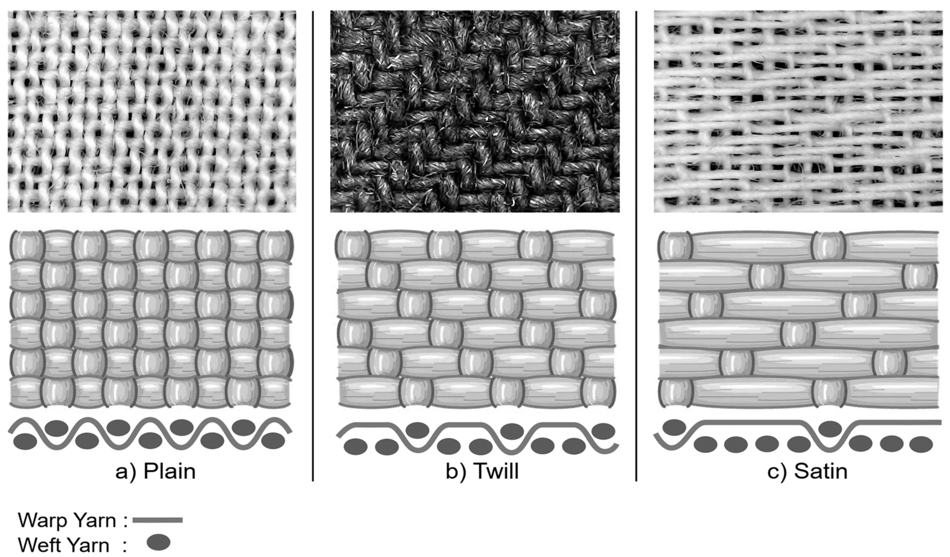
The collected data set is not enough to cover all textile products, therefore, there are some limitations and assumptions in the materials and methods followed during the collection of the woven fabric image data set. In this study, 130 images of fabrics were captured using a digital handheld microscope with resolution of 640 × 480 pixels. The microscope used was purchased [18]. The image size was set to 5 mm × 4 mm. Illumination was carried out from behind the microscope. The fabrics are manufactured in three primary texture types as presented in Figure 1: plain, twill, and satin. In the sample selection, we aimed to have samples of various colors and weft–warp density. The fabric samples have not been utilized or deformed; the imagery is acquired from a small area (5 mm × 4 mm) through a transparent plastic attachment at the tip of the microscope, which ensures that the fabric remains in a uniform state. Consequently, it can be asserted that there is virtually no occurrence of crimp or skew in the fabric images compared to manual measurements. Thickness refers to the distance between the top and bottom surfaces of a fabric, measured from the front surface to the back surface. This is of significance for ready-to-wear garment manufacturers because it impacts processes such as cutting, sewing, transportation, and storage. In this study, image data were collected from single-layer outerwear fabrics. Obtaining information about the lower layers in multi-layer fabrics is not possible with top-view cameras. The thickness of the used fabrics varies depending on factors such as weft density, warp density, and weight. The study is limited to single-layer fabrics with a thickness range of approximately 0.1 mm to 1 mm. The measurement system is performed on the fabric surface and does not cover backlighting; thus thickness information cannot be obtained from the images. The fabrics used in the study were made of 70% to 100% cotton yarn. Other compositions of fabrics are polyester or elastane. The collected images consist of 50 samples of plain texture, 41 samples of satin texture, and 39 samples of twill texture. The weight of the fabrics in grams per square meter (g/m²) has been presented as the specific mass value. This value is associated with parameters such as yarn composition, weft, and warp counts, as well as pore size values.

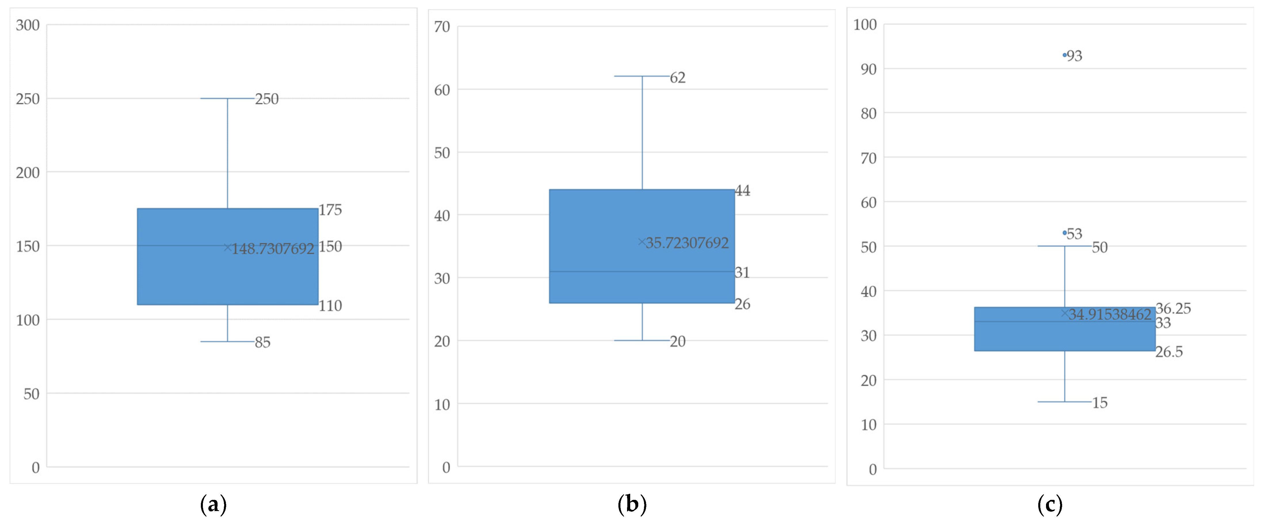
The specific mass values of the collected images vary in the range of (85–250) and are illustrated in Figure 2a. The weft count represents the number of horizontal threads per centimeter (cm) in the fabrics. In the collected images, the weft count varies in the range of (15–93), and its distribution is shown in Figure 2b. The warp count represents the number of vertical threads per centimeter (cm) in the fabrics. In the collected images, the warp count varies in the range of (20–62), and its distribution is depicted in Figure 2c.

2.2. Texture Feature Extraction

In this study, feature extraction was performed using the GLCM, LBP, GFB, and IFV methods as presented in

Table 2. Texture Feature Extraction Methods and Parameters.

Feature Extraction	Parameters
GLCM	Since memory and time parameters were not the primary goal of this paper, GLCM was used with 256 levels. Additionally, co-occurrences at 0, 45, and 90 degrees at a distance of one pixel were processed. Contrast, Dissimilarity, Homogeneity, Energy, and Correlation were used as attributes.
LBP	Half of the window width used for feature extraction in the case of LBP (i.e., 80) was designated as the LBP radius. Feature extraction for LBP was performed with point configurations of 20, 40, and 80.
GFB	Gabor filter bank feature extraction involves calculating the mean, variance, and peak-to-peak value of pixels in the filtered image obtained by applying different Gabor filters to the input image.
IFV	A step size of 20 pixels and a frame width of 10 pixels were chosen.

, employing a sliding window approach with dimensions of 160 × 160 and a stride of 80 on microscope images captured at 640 × 480 resolution. The images taken from the camera were converted to gray scale only before feature extraction.

2.2.1. Gray-Level Co-occurrence Matrix Feature Extraction

The Gray-Level Co-occurrence Matrix (GLCM) is a second-order statistical technique employed in the extraction of textural attributes from images. The underlying principle of GLCM feature extraction involves the creation of a co-occurrence matrix for a designated segment of the image, from which a multitude of characteristics can be derived [19]. GLCM is widely employed in the domain of textile defect detection [19,20,21,22]. It has been reported that GLCM can outperform methods like GFB or LBP in certain scenarios of fabric defect detection [21,23,24].

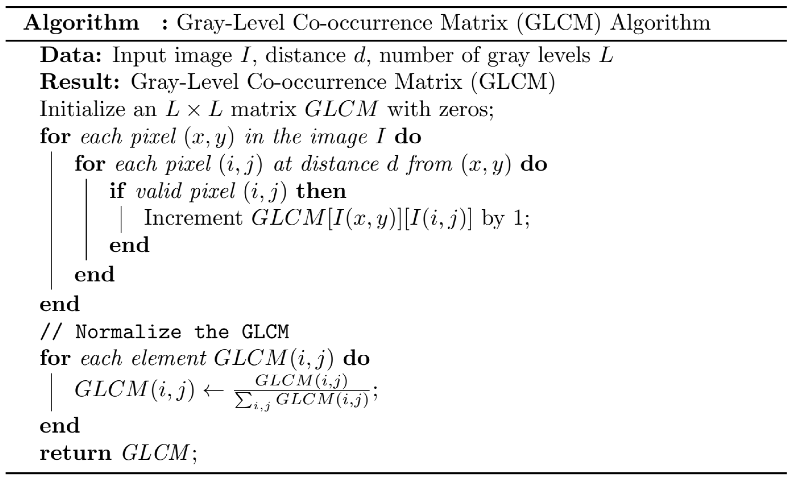
The GLCM algorithm, which is shown in Figure 3, is a method used to compute the Gray-Level Co-occurrence Matrix of an image I. The GLCM stores the frequency of each pair of adjacent pixels in the image. First, it initializes an LxL matrix GLCM with zeros, where L is the number of gray levels in the image. Then, it loops over each pixel (x, y) in the image and for each pixel (i, j) at distance d from (x, y), it checks if (i, j) is a valid pixel. If so, it increments GLCM [I(x, y)][I(i, j)] by 1. After the loop ends, it normalizes the GLCM by dividing each element by the sum of all elements in the matrix. Finally, it returns the GLCM as the result. After computing the GLCM matrix, the most common approach is to calculate various features, such as contrast, dissimilarity, homogeneity, energy, and correlation [25]. These features can be used to describe the texture of the image and compare different patches. In addition, if GLCM applications use high-dimensional frames, it requires a large amount of memory. This increases the feature extraction processing time. To overcome this situation, the number of gray levels can be reduced by accepting information loss and thus the size of the matrix can be reduced.

2.2.2. Local Binary Pattern Feature Extraction

The Local Binary Pattern (LBP) technique, which is prevalent in the domain of textile defect detection, has found extensive application in various domains, including facial recognition and texture categorization [23,24,26,27]. The LBP algorithm, which is shown in Figure 4, first initializes an empty LBP image with the same dimensions as the input image. Then, it loops over each pixel (x, y) in the input image and for each pixel (i, j) at distance R from (x, y), it computes the coordinates of the i-th neighbor pixel (x_i, y_i) on a circle of radius R centered at (x, y). It also obtains the pixel value P_i at location (x_i, y_i). Next, it checks if P_i ≥ C, where C is the pixel value at location (x, y). If so, it appends 1 to a binary list lbp_code that stores binary values for each pixel. Otherwise, it appends 0 to the list. After the loop ends, it converts the binary list lbp_code to a decimal value by counting how many 1s are in the list. It then sets the LBP value at location (x, y) in the LBP image to the computed decimal value. Finally, it returns the LBP image as the result. The outcome of the procedure entails the summation of products of matrix elements. In certain contexts, it is exclusively employed for the purpose of binarization, omitting the multiplication phase. The primary merits of employing the LBP technique encompass its straightforward implementation and minimal computational overhead. Nevertheless, this approach exhibits a notably diminished efficacy when confronted with variations in illumination and alterations in image orientation.

2.2.3. Gabor Filter Bank Feature Extraction

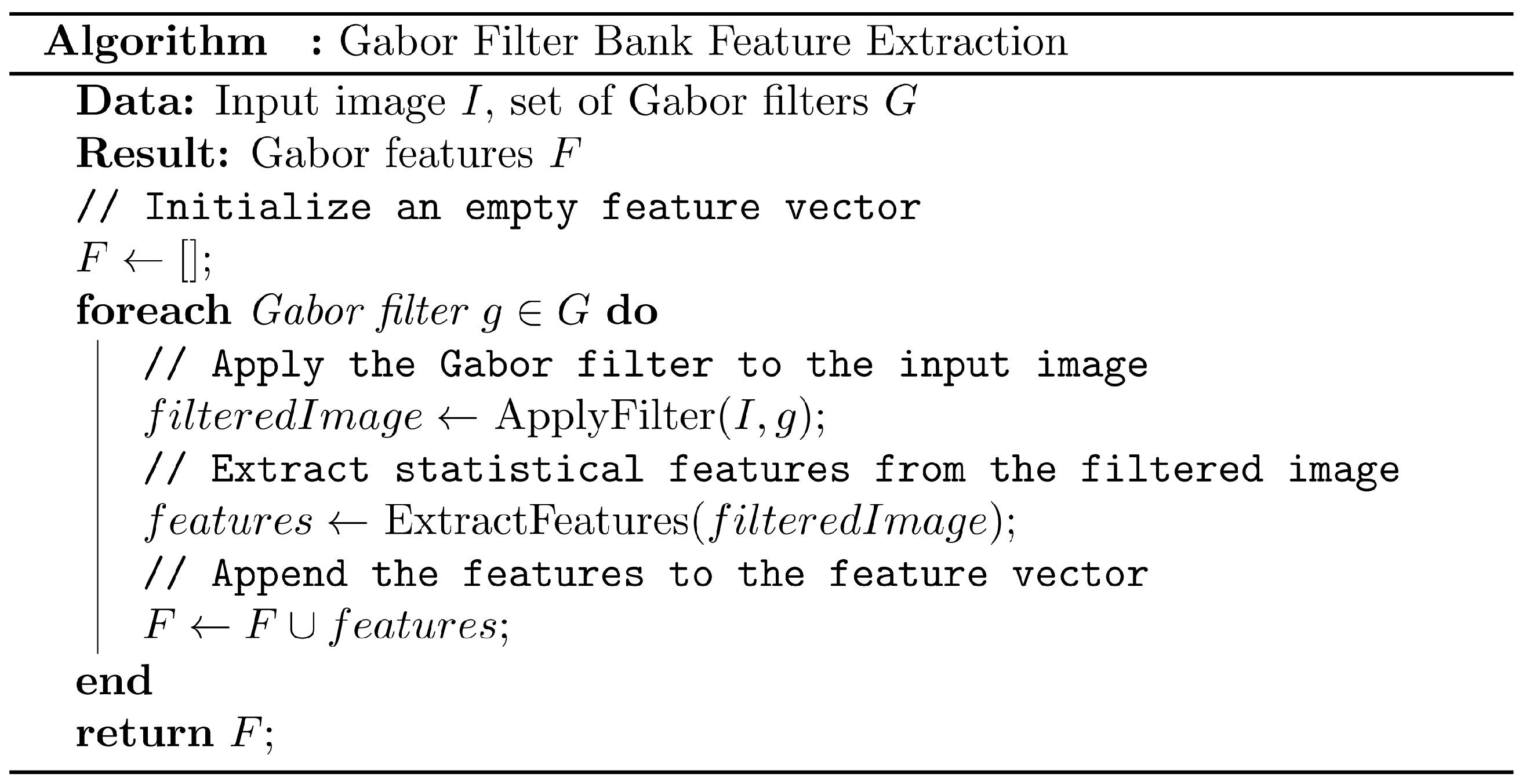
The process of feature extraction through the utilization of the Gabor Filter Bank (GFB) entails the construction of a comprehensive array of Gabor filters, each characterized by diverse parameters. This approach is employed to encapsulate the frequency and orientation attributes of an image, effectively emulating the function of edge detection. Gabor filters, which belong to the wavelet filter category, exhibit distinguishing features such as a Gaussian envelope and sinusoidal modulation. These filters are intentionally engineered to emulate the functionality of the human visual system, resulting in the generation of seamlessly continuous responses. The GFB algorithm, which is shown in Figure 5, first initializes an empty feature vector F with zeros. Then, it loops over each Gabor filter g$ϵ$ G, which is a set of Gabor filters that are designed to capture different aspects of the image. Next, it applies the Gabor filter to the input image I and stores the filtered image filteredImage. After that, it extracts statistical features from the filtered image filteredImage, such as mean, variance, entropy, etc. Finally, it appends the features to the feature vector F by using the union operator. Finally, it returns the feature vector F as the result. The feature vector F can be used to measure the similarity between two images by computing their dot product. A higher dot product means more similar pixels and vice versa.

A Gabor Filter in the realm of two-dimensional signal processing comprises two fundamental components, delineated in Equation (1). These components, the carrier, and the envelope, are distinctly defined in Equations (2) and (3), correspondingly. The carrier function is characterized by a two-dimensional sinusoidal waveform, with wavelength denoted as λ and a phase offset value φ. Meanwhile, the Envelope Function can be conceptualized as an equation representing a circle, the aspect ratio of which can be adjusted using the variable γ. To determine the x’ and y’ values, Equations (4) and (5) are employed, respectively, with the variable θ signifying the orientation angle. By manipulating these parameters integral to the Gabor filter, a myriad of filter configurations can be generated. Subsequently, these filters are convolved with predefined windows across the image and transformed into feature vectors. This method has been harnessed in diverse applications, notably within domains such as fabric defect classification [21,27,28,29].

$$g\left(x,y,\sigma , \theta ,\lambda , \gamma , \phi \right)=s\left(x,y,\theta ,\sigma , \gamma \right)\times w_r\left(x,y,\theta ,\lambda , \phi \right)$$

(1)

$$wr\left(x,y,\theta ,\lambda , \phi \right)=e^{\left[-\frac{x{\prime }^2+{\gamma }^{2}y{\prime }^2}{2{\sigma }^2}\right]}$$

(2)

$$s\left(x,y,\sigma , \gamma \right)=e^{\left[i\left(2\pi \frac{x\prime }{\lambda }+\phi \right)\right]}$$

(3)

$$x\prime =x\cos \left(\theta \right)+y\sin \left(\theta \right)$$

(4)

$$y\prime =-x\sin \left(\theta \right)+y\cos \left(\theta \right)$$

(5)

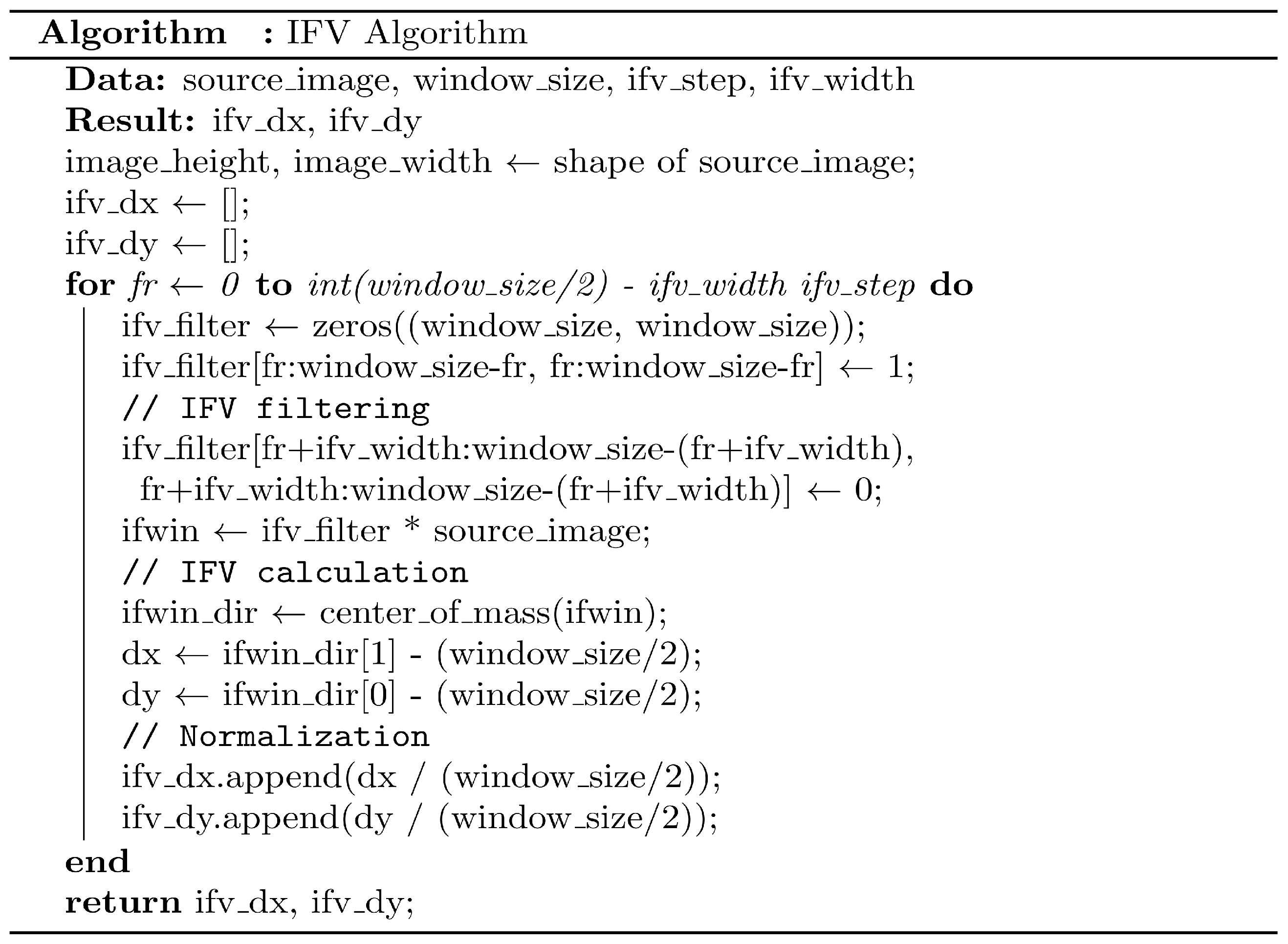
2.2.4. Intertwined Frame Vector

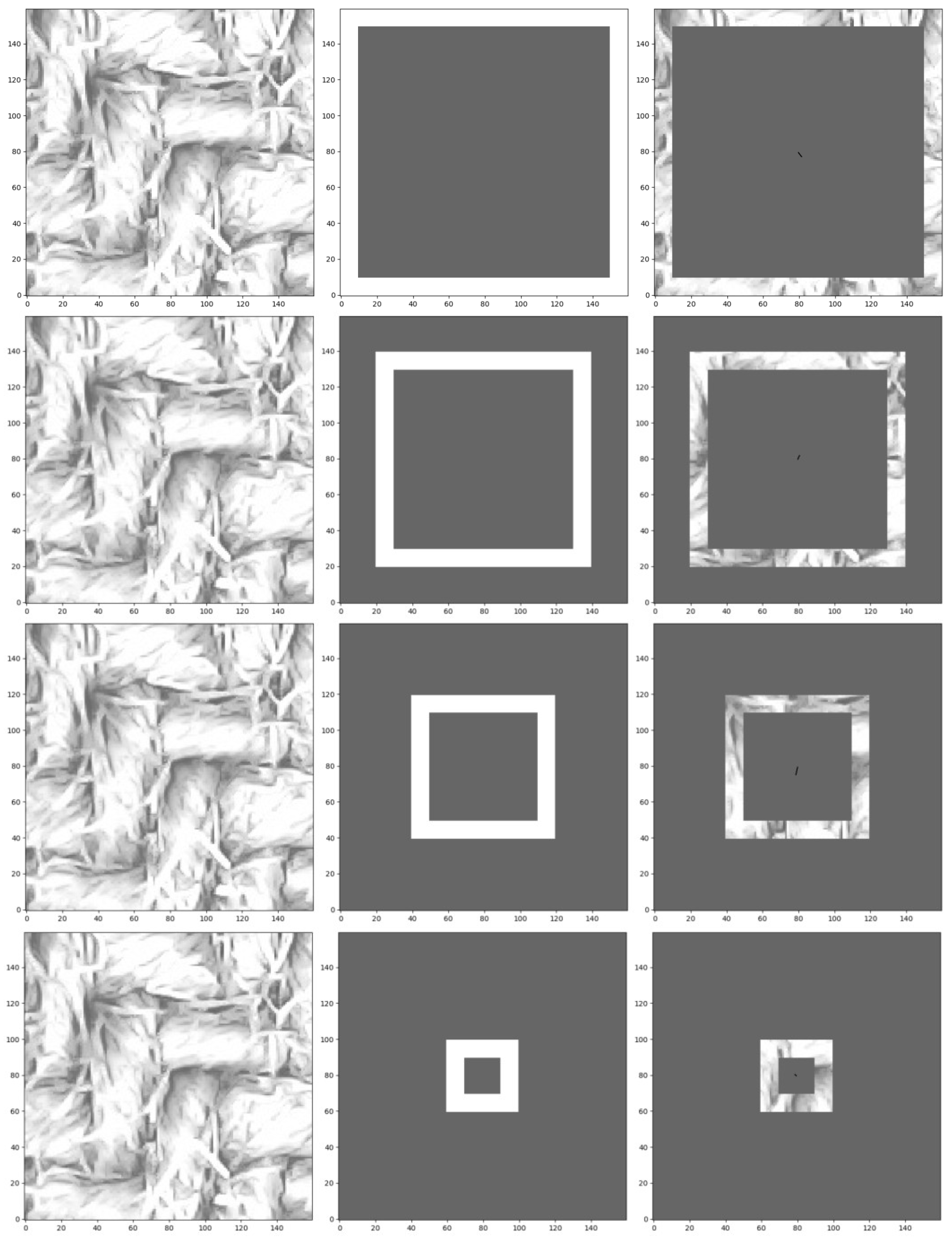
The Intertwined Frame Vector (IFV) method is a feature extraction technique that calculates the weighted centroids of multiple nested frames over a texture and draws a vector from the center of the image to the weighted centroid. In this algorithm, which is presented in Figure 6, the frame step and frame thickness are first determined. Then, iteratively, the centroids of the frames are computed, and a vector is drawn from the center of the window to the weighted centroid. The vector is normalized with respect to the window size, and, for each window, the endpoint coordinates (dx, dy) of the vector or the vector’s angle and magnitude are used as features. Figure 7 illustrates the IFV outputs for a 160 × 160 pixel fabric image with a step size of 20 and a window width of 10. When IFV is used for fabric defect detection with small-sized sliding windows, it has shown successful results in terms of both performance and processing speed [30].

2.3. Machine Learning for Texture Classifcation and Weaving Parameter Regression

The utilization of the dataset with Machine Learning begins with the feature extraction process, as demonstrated in Figure 8. For each window using GLCM, LBP, GFB, and IFV methods along with the sliding window technique, 458 features are extracted. These 458 feature columns are employed as input for Machine Learning. On top of these columns, the output for fabric-texture-type classification and the weaving parameters’, specific mass, weft, and warp, columns for woven fabric are added as regression outputs, constructing the general dataset in a tabular format. In the subsequent step, the dataset is split into a 70% training and a 30% testing portion. The texture classification task within the dataset is defined as having three classes: plain, twill, and satin. Accuracy is employed as the primary performance evaluation criterion for texture classification, and, after training, the selected model is tested to obtain the results. For regression tasks, models generated in terms of performance metrics are compared, and ultimately the chosen models are evaluated with the test data to obtain the results.

2.3.1. Random Forest

The Random Forest (RF) algorithm stands as a robust ensemble-based machine learning methodology employed for the resolution of both classification and regression tasks [31,32]. RF first creates multiple decision trees. Each tree creates a tree structure by splitting the data using a subset of random features. This subset selection ensures that each tree is different from each other. Each decision tree is trained using data. These trees classify or predict data based on input features. The trained decision trees are used to further classify or predict new data. For classification problems, the class is predicted based on the decision of most trees. For regression problems, the average of the predictions of most of the trees is taken. RF produces a more reliable and stable result by combining the predictions of each tree. It reduces the risk of RF overfitting, so it is generally high performing. It can process many features and automatically select important features, so its explainability is high. RF is resistant to outlier values. However, in large data sets or when many trees are used, the computational cost generally increases. RF may produce less understandable and interpretable results than decision trees. In this study, 20 trees were used as RF parameters and a subset smaller than 5 was chosen as non-dividing.

2.3.2. Extreme Gradient Boosting

Extreme Gradient Boosting (XGBoost), an enhanced iteration of the Gradient Boosting method, is a versatile ensemble machine learning algorithm employed for both regression and classification problems, fundamentally grounded in tree-based learning principles [33,34]. Initially, it creates numerous decision trees referred to as weak learners. These trees are used to capture the complexity of the dataset by partitioning data points based on certain features. The predictions of the first tree are compared to the actual values to compute errors. Subsequently, the next tree is constructed to try to correct these errors. The second tree aims to reduce the errors made by the first tree. Trees are added sequentially, and predictions accumulate. As each tree is added, weights are assigned to the predictions of previous trees, optimizing the error correction process. XGBoost incorporates various regularization techniques to prevent overfitting. XGBoost is a high-performance algorithm and often delivers successful results in competitions and industrial applications. Thanks to its regularization techniques, it is more robust against overfitting. However, optimizing an XGBoost model may require hyperparameter tuning, which can be time consuming. There is a risk of overfitting in small datasets. In this study, the XGBoost library was utilized for XGBoost, with the following hyperparameters: 100 trees, a learning rate of 0.3, a lambda value of 1, and a tree depth of 7.

2.3.3. Multilayer Perceptron

The Multilayer Perceptron (MLP) is a class of artificial neural networks primarily employed for solving complex problems, characterized by its multiple layers of artificial neurons, each layer processing input data to produce the desired output [35,36]. It typically includes at least three layers: an input layer, at least one hidden layer, and an output layer. Each neuron calculates the weighted sum of inputs from the neurons in the previous layer and then passes this sum through an activation function. Data enter the MLP through the input layer, with each input neuron representing a data feature. The hidden layers represent the learning and complexity of the data. Each neuron in these layers takes the weighted sum from the neurons in the previous layer, applies an activation function, and processes this information by passing it to the next layer. The output layer is responsible for producing results. In classification problems, each output neuron represents a class or label, while in regression problems, it predicts a continuous value. When MLP is used to solve regression problems, the neurons in the output layer represent the regression target. MLP has a high learning capacity and is versatile, making it suitable for various problems. Deep networks, which are popular today, consist of MLPs with numerous hidden layers and can better model complex problems as the depth increases [37]. However, as problem complexity increases, training time and real-time processing requirements can also grow due to the larger network size. The design of MLPs can be data-intensive for some datasets, posing a risk of overfitting, thus necessitating proper regularization and redesign. As the network and architecture grow, parameter tuning and architecture selection for MLP models become more challenging. Additionally, artificial neural networks, including MLPs, are considered black boxes in terms of explainability, despite their high performance in complex problems. In this study, the architecture of the MLP used consisted of hidden layers with 500, 100, and 50 neurons, respectively, following the input layer. Rectified linear unit (ReLu) was chosen as the activation function, and Adam was selected as the solver. The number of iterations for MLP was set to 500.

2.4. Machine Learning Performance Evaluation

The dataset underwent an initial division into two segments, with 70% designated for training purposes and the remaining 30% set aside for testing. The training dataset serves as the repository of information employed for training the model, whereas the test dataset is exclusively reserved for appraising the model’s efficacy. To enhance the training process, the training dataset was subsequently subdivided into smaller subsets utilizing 5-fold cross-validation, facilitating the undertaking of model selection.

The model used for texture classification is trained on the training dataset, and the results obtained after the 5-fold cross-validation process are evaluated. To measure classification performance, accuracy, F1 score, precision, and recall performance metrics, as presented in

Table 3. Classification Metrics.

Metric	Explanation	Equation
Accuracy	It measures the accuracy of classification and shows the ratio of correctly predicted instances to the total data.	$A=\frac{TP + TN}{TP + TN + FP + FN}$
Precision	It indicates the ratio of true positives to the instances that were predicted as positive.	$P=\frac{TP}{TP + FP}$
Recall	It shows how many of the truly positive instances were correctly predicted as positive.	$R=\frac{TP}{TP + FN}$
F1 Score	It is the harmonic mean of precision and recall metrics and provides information about classification balance.	$F1=\frac{2 \times P \times R }{P+R}$

, are used. In a three-class confusion matrix, the terms True Positives (TP), True Negatives (TN), False Positives (FP), and False Negatives (FN) are key metrics for evaluating the performance of a classification model in a multi-class context. True Positives represent instances correctly classified as belonging to a specific class, while True Negatives denote instances accurately classified as not belonging to that class. False Positives are instances incorrectly identified as belonging to a class they do not actually belong to, and False Negatives are instances erroneously labeled as not belonging to a class when they, in fact, do belong. These metrics provide a detailed assessment of the model’s ability to make accurate and erroneous predictions within each class, facilitating a deeper understanding of its performance in multi-class classification scenarios.

In this study, for regression tasks involving the estimation of specific mass, weft, and warp values, mean absolute error (MAE) and coefficient of determination (R²) metrics are used. These metrics are summarized in

Table 4. Regression Metrics.

Metric	Explanation	Equation
MAE	It represents the arithmetic mean of the absolute disparities between empirically recorded data points and their corresponding projected values.	$MAE=\frac{\sum \left|y-\widehat{y}\right|}{n}$
R2	This quantitative metric serves as an analytical tool delineating the extent to which the independent variables within a regression model elucidate the variability in the dependent variable. It indicates that the model is better as it approaches 1.	$R^2=1-\frac{\sum {\left(y-\widehat{y}\right)}^2}{\sum {\left(y-\overline{y}\right)}^2}$

. In this table, “y” represents the actual dependent variable values, “ŷ” signifies the predicted dependent variable values by the model, and “ȳ” is the mean of the actual dependent variable values.

3. Results and Discussion

3.1. Texture Classification

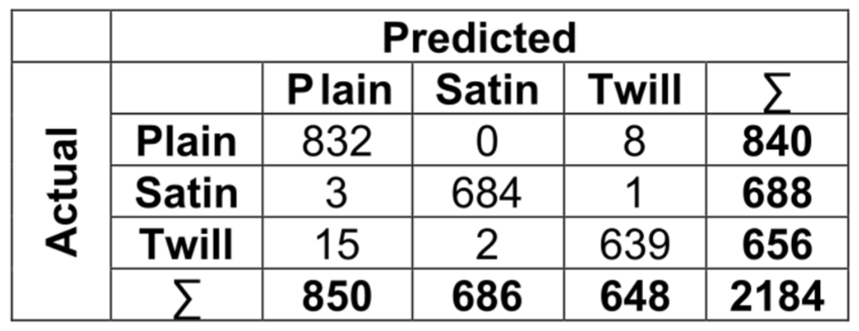
The accuracy, F1 score, precision, and recall performance metrics obtained for training in texture-type prediction are presented in

Table 5. Machine Learning algorithm training performance on texture classification.

Learning Algorithm	Time		Performance Metrics
	Train	Test	Accuracy	F1	Precision	Recall
XGBoost	14.739	0.094	0.987	0.987	0.987	0.987
MLP	41.123	0.820	0.987	0.987	0.987	0.987
RF	1.747	0.336	0.979	0.979	0.979	0.979

. XGBoost has produced the most successful model with an accuracy of 0.987. The confusion matrix for MLP on the training data is shown in Figure 9. According to the confusion matrix, the texture “twill” is the one that XGBoost model confused the most. Out of seventeen instances that were twill, fifteen were predicted as plain, and two were predicted as satin. This situation is believed to be due to the fact that twill texture resembles both satin and plain textures the most.

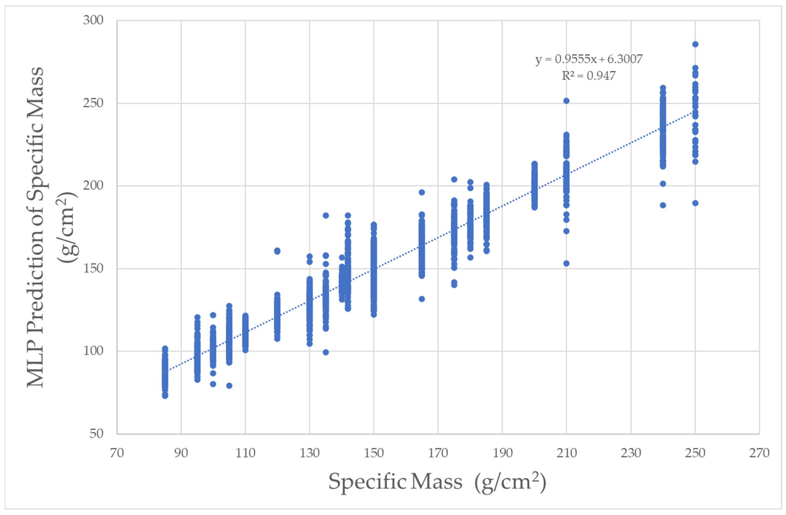
3.2. Specific Mass Prediction

The MAE and R² values obtained for specific mass prediction in the training set are presented in

Table 6. Machine Learning algorithm training performance on specific mass prediction.

Learning Algorithm	Time		Performance Metrics
	Train	Test	MAE	R2
MLP	210.239	0.660	6.739	0.947
RF	19.810	0.343	5.121	0.936
XGBoost	15.285	0.026	5.761	0.932

. Regarding MAE, the RF algorithm has the lowest error value at 5.121 g/cm². When the algorithms used in the study are compared in terms of R², the highest value is 0.947, achieved with the MLP algorithm. The predictions for the training and test values using MLP are shown in Figure 10 and Figure 11, respectively. For MLP, the R² value for prediction using the test data is 0.956.

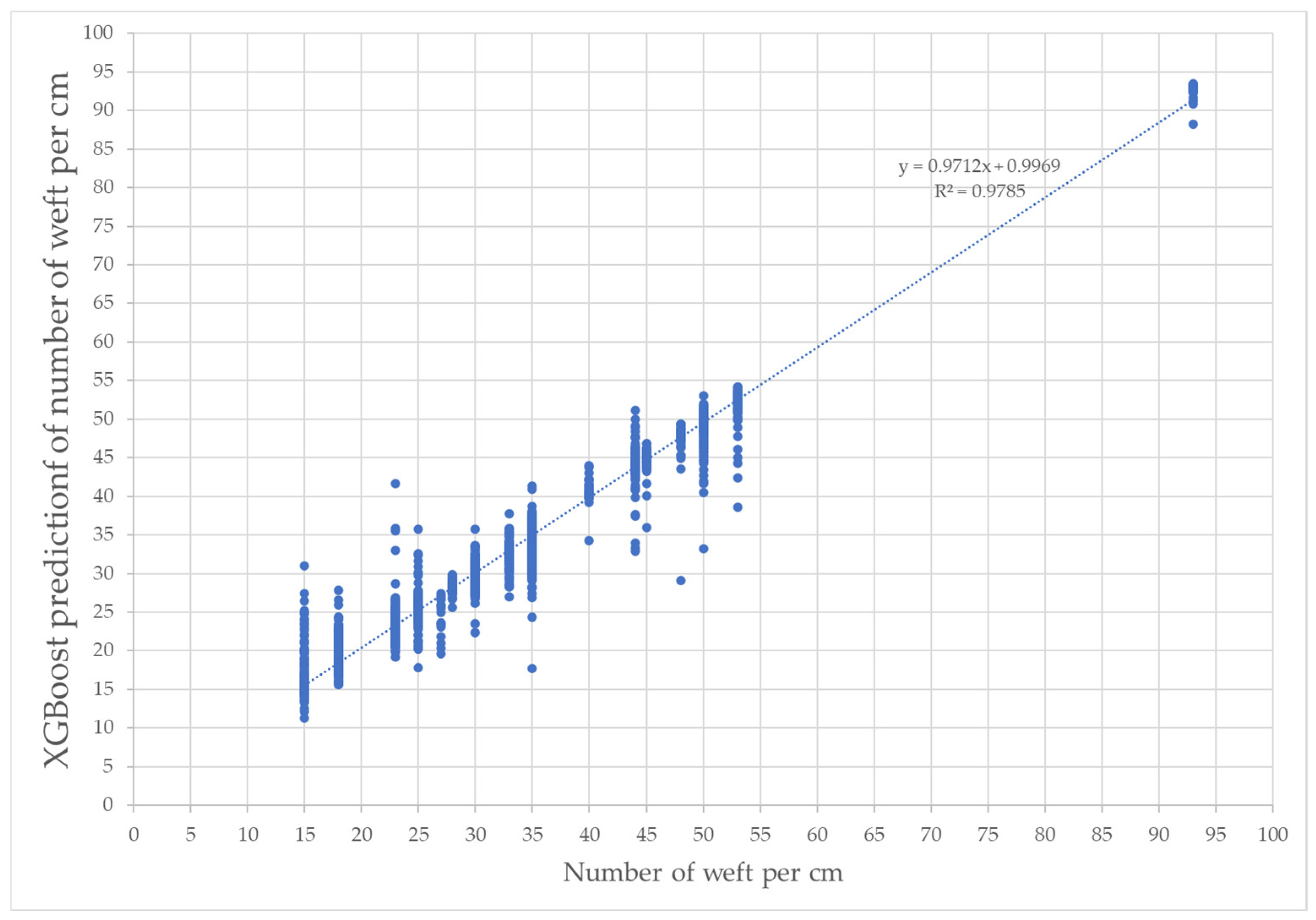
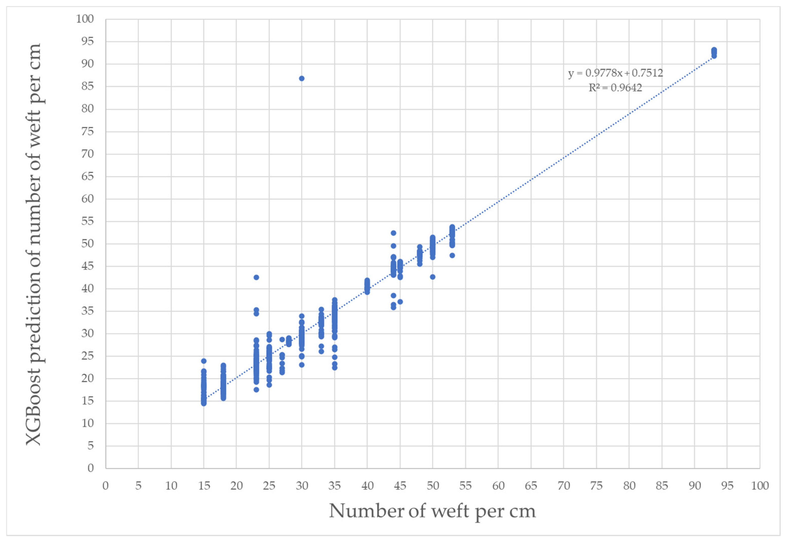
3.3. Weft Density Prediction

The MAE and R² values obtained for weft prediction in the training set are presented in

Table 7. Machine Learning algorithm training performance on weft prediction.

Learning Algorithm	Time		Performance Metrics
	Train	Test	MAE	R2
XGBoost	14.299	0.034	1.213	0.978
MLP	156.459	0.803	1.765	0.973
RF	18.683	0.323	1.287	0.972

. In terms of MAE, XGBoost has the lowest error value at 1.213 weft yarn/cm. When the algorithms used in the study are compared in terms of R², the highest value is 0.978, achieved with the XGBoost algorithm. The predictions for the training and test values using XGBoost are shown in Figure 12 and Figure 13, respectively. For XGBoost, the R² value for prediction using the test data is 0.964.

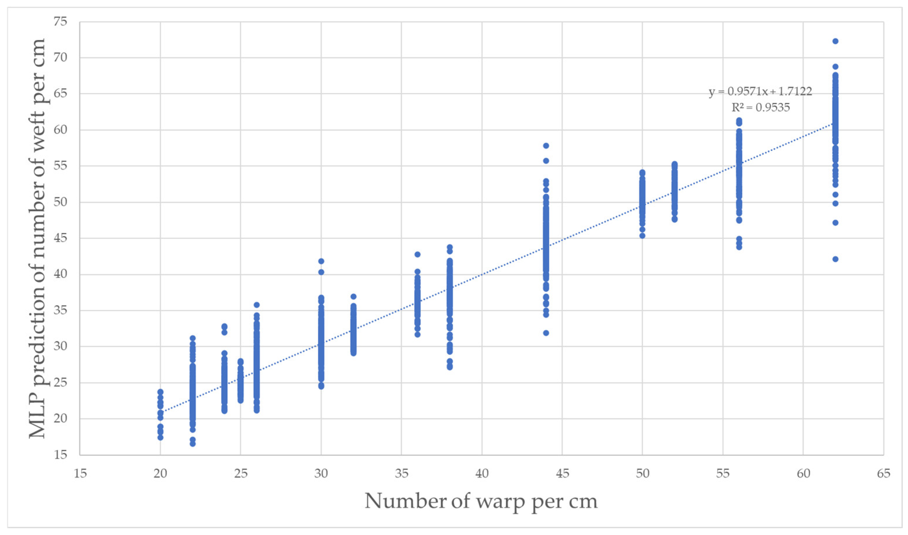
3.4. Warp Density Prediction

The MAE and R² values obtained for warp prediction in the training set are presented in

Table 8. Machine Learning algorithm training performance on warp prediction.

Learning Algorithm	Time		Performance Metrics
	Train	Test	MAE	R2
MLP	6.963	2.639	1.833	0.953
RF	9.180	3.030	1.450	0.938
XGBoost	9.819	3.134	1.547	0.934

. In terms of MAE, MLP has the lowest error value at 2.639 warp yarn/cm. When the algorithms used in the study are compared in terms of R², the highest value is 0.953, achieved with the MLP algorithm. The predictions for the training and test values using MLP are shown in Figure 14 and Figure 15, respectively. For MLP, the R² value for prediction using the test data is 0.976.

4. Conclusions

This paper introduces a dataset and proposes a method aimed at enhancing texture detection and weaving parameter prediction in the textile industry. By leveraging a low-cost microscopy fabric dataset and machine learning techniques, it becomes possible to achieve more precise and efficient outcomes in textile production. The objective is to take a significant step towards the textile industry’s sustainability goals and product quality improvement.

In this study, texture type, specific mass, weft, and warp parameters for fabric images obtained using a low-cost digital hand-held microscope were manually labeled. Various texture feature extraction methods, including GLCM, GFB, LBP, and IFV, were applied to the acquired dataset, resulting in the creation of a tabular dataset with four hundred and fifty-eight inputs and four outputs. Machine learning algorithms such as RF, XGBoost, and MLP were employed. The findings indicate that the XGBoost algorithm achieved an accuracy of 0.987 for the texture classification task. For specific mass prediction, the lowest MAE value of 5.121 g/cm was obtained using RF. Regarding weft prediction, the lowest MAE value of 1.213 yarn/cm was achieved using XGBoost. For warp prediction, the lowest MAE value of 2.639 yarn/cm was obtained using MLP. Comparing the results with manual measurements, it can be observed that the errors in specific mass, weft, and warp predictions were lower using the proposed methods. In texture type detection, a high accuracy of 0.987 was achieved, indicating the success of the proposed approach.

Future prospects for this research involve the incorporation of an image-stitching function to enable the collection of larger images. This expansion allows for the exploration of texture recognition in fabrics characterized by mixed textures, which presents a significant challenge in the textile industry. Furthermore, the estimation of weaving parameters holds substantial promise in terms of time and resource savings for textile companies, especially within the order processing and quality control processes, thereby contributing to sustainability objectives. Given the cost-effectiveness of the data collection device and ease of image acquisition, the intention is to assemble a more comprehensive dataset in the future by incorporating data from diverse fabric types. This approach not only holds relevance in the clothing sector, where textile products are used directly, but also exhibits potential applicability in quality control across various sectors, such as furniture, automotive, military, healthcare, and construction.

This study underscores the paramount significance of integrating artificial intelligence technology across the various stages of the textile industry. Specifically, the application of texture and weave parameter estimation stands to optimize resource utilization by diminishing trial-and-error procedures conducted manually. Reduced consumption of raw materials aligns with the preservation of natural resources, while the automation of fabric analysis enhances worker productivity and fosters improvements in worker health and safety. Consequently, artificial intelligence technology exerts a considerable influence on sustainability, efficiency, worker well-being, and data analysis within the textile industry. These advancements are poised to yield positive outcomes from both environmental and societal standpoints.

References

- Niwa, M. The Importance of Clothing Science and Prospects for the Future. Int. J. Cloth. Sci. Technol. 2002, 14, 238–246. [Google Scholar] [CrossRef]
- Chattopadhyay, R. Design of Apparel Fabrics: Role of Fibre, Yarn and Fabric Parameters on Its Functional Attributes. J. Text. Eng. 2008, 54, 179–190. [Google Scholar] [CrossRef]
- Yuldoshev, N.; Tursunov, B.; Qozoqov, S. Use of Artificial Intelligence Methods in Operational Planning of Textile Production. J. Process Manag. New Technol. 2018, 6, 41–51. [Google Scholar] [CrossRef]
- Seçkin, M.; Seçkin, A.Ç.; Coşkun, A. Production Fault Simulation and Forecasting from Time Series Data with Machine Learning in Glove Textile Industry. J. Eng. Fibers Fabr. 2019, 14, 155892501988346. [Google Scholar] [CrossRef]
- Naseem, S.; Kashif, L.; Mahmood, S. Role of Computer Programming in Processing and Management of Textile Industry—A Review. Asia Pac. J. Emerg. Mark. 2020, 4, 79–92. [Google Scholar]
- Sikka, M.P.; Sarkar, A.; Garg, S. Artificial Intelligence (AI) in Textile Industry Operational Modernization. Res. J. Text. Appar. 2022. ahead-of-print. [Google Scholar] [CrossRef]
- Schulz-Mirbach, H. Ein Referenzdatensatz zur Evaluierung von Sichtprüfungsverfahren für Textiloberflächen; TU Hamburg: Hamburg, Germany, 1996. [Google Scholar]
- Cimpoi, M.; Maji, S.; Kokkinos, I.; Mohamed, S.; Vedaldi, A. Describing Textures in the Wild. In Proceedings of the IEEE Conference on Computer Vision and Pattern Recognition, Columbus, OH, USA, 23–28 June 2014; pp. 3606–3613. [Google Scholar]
- Kampouris, C.; Zafeiriou, S.; Ghosh, A.; Malassiotis, S. Fine-Grained Material Classification Using Micro-Geometry and Reflectance. In Proceedings of the Computer Vision–ECCV 2016, Amsterdam, The Netherlands, 11–14 October 2016; Leibe, B., Matas, J., Sebe, N., Welling, M., Eds.; Springer International Publishing: Cham, Switzerland, 2016; pp. 778–792. [Google Scholar]
- Özgenel, Ç.F.; Sorguç, A.G. Performance Comparison of Pretrained Convolutional Neural Networks on Crack Detection in Buildings. In Proceedings of the ISARC 2018, Proceedings of the International Symposium on Automation and Robotics in Construction, Berlin, Germany, 20–25 July 2018; IAARC Publications: Berlin, Germany, 2018; Volume 35, pp. 1–8. [Google Scholar]
- Silvestre-Blanes, J.; Albero Albero, T.; Miralles, I.; Pérez-Llorens, R.; Moreno, J. A Public Fabric Database for Defect Detection Methods and Results. Autex Res. J. 2019, 19, 363–374. [Google Scholar] [CrossRef]
- Zhang, H.; Zhang, W.; Wang, Y.; Lu, S.; Yao, L.; Chen, X. Colour-Patterned Fabric-Defect Detection Using Unsupervised and Memorial Defect-Free Features. Color. Technol. 2022, 138, 602–620. [Google Scholar] [CrossRef]
- TILDA Textile Texture-Database. Available online: https://lmb.informatik.uni-freiburg.de/resources/datasets/tilda.en.html (accessed on 18 September 2023).
- Describable Textures Dataset. Available online: https://www.robots.ox.ac.uk/~vgg/data/dtd/ (accessed on 19 September 2023).
- The Fabrics Dataset. Available online: https://ibug.doc.ic.ac.uk/resources/fabrics/ (accessed on 18 September 2023).
- Özgenel, Ç.F. Concrete Crack Images for Classification. 2019. Available online: https://data.mendeley.com/datasets/5y9wdsg2zt/2 (accessed on 18 September 2023).
- Aitex Fabric Image Database. Available online: https://www.aitex.es/afid/ (accessed on 18 September 2023).
- USB Microscope Camera 1000X. Available online: https://www.amazon.com/Microscope-Digital-Carrying-Compatible-Portable/dp/B085XZVFGT/ref=sr_1_1_sspa?c=ts&keywords=Lab%2BHandheld%2BDigital%2BMicroscopes&qid=1697121376&s=photo&sr=1-1-spons&ts_id=2742273011&sp_csd=d2lkZ2V0TmFtZT1zcF9hdGY&th=1 (accessed on 12 October 2023).
- Haralick, R.M.; Shanmugam, K.; Dinstein, I. Textural Features for Image Classification. IEEE Trans. Syst. Man Cybern. 1973, SMC-3, 610–621. [Google Scholar] [CrossRef]
- Zhang, X.D.; Huang, X.B. Fabric’s Filling Bar Defect Detection Based on Grey-Level Co-Occurrence Matrix and Robust Mahalanobis Distance. J. Donghua Univ. Nat. Sci. 2009, 35, 691–698. [Google Scholar]
- Raheja, J.L.; Kumar, S.; Chaudhary, A. Fabric Defect Detection Based on GLCM and Gabor Filter: A Comparison. Optik 2013, 124, 6469–6474. [Google Scholar] [CrossRef]
- Zhu, D.; Pan, R.; Gao, W.; Zhang, J. Yarn-Dyed Fabric Defect Detection Based on Autocorrelation Function and GLCM. Autex Res. J. 2015, 15, 226–232. [Google Scholar] [CrossRef]
- Zhang, L.; Jing, J.; Zhang, H. Fabric Defect Classification Based on LBP and GLCM. J. Fiber Bioeng. Inform. 2015, 8, 81–89. [Google Scholar] [CrossRef]
- Kaynar, O.; Işik, Y.E.; Görmez, Y.; Demirkoparan, F. Fabric Defect Detection with LBP-GLMC. In Proceedings of the 2017 International Artificial Intelligence and Data Processing Symposium (IDAP), Malatya, Turkey, 16–17 September 2017; pp. 1–5. [Google Scholar]
- GLCM Texture: A Tutorial v. 3.0. March 2017. Available online: https://prism.ucalgary.ca/items/8833a1fc-5efb-4b9b-93a6-ac4ff268091c (accessed on 18 September 2023).
- Jing, J.; Zhang, Z.; Kang, X.; Jia, J. Objective Evaluation of Fabric Pilling Based on Wavelet Transform and the Local Binary Pattern. Text. Res. J. 2012, 82, 1880–1887. [Google Scholar] [CrossRef]
- Jing, J.; Zhang, H.; Wang, J.; Li, P.; Jia, J. Fabric Defect Detection Using Gabor Filters and Defect Classification Based on LBP and Tamura Method. J. Text. Inst. 2013, 104, 18–27. [Google Scholar] [CrossRef]
- Shu, Y.; Tan, Z. Fabric Defects Automatic Detection Using Gabor Filters. In Proceedings of the Fifth World Congress on Intelligent Control and Automation (IEEE Cat. No.04EX788), Hangzhou, China, 15–19 June 2004; Volume 4, pp. 3378–3380. [Google Scholar]
- Han, R.; Zhang, L. Fabric Defect Detection Method Based on Gabor Filter Mask. In Proceedings of the 2009 WRI Global Congress on Intelligent Systems, Xiamen, China, 19–21 May 2009; Volume 3, pp. 184–188. [Google Scholar]
- Seçkin, A.Ç.; Seçkin, M. Detection of Fabric Defects with Intertwined Frame Vector Feature Extraction. Alex. Eng. J. 2022, 61, 2887–2898. [Google Scholar] [CrossRef]
- Safavian, S.R.; Landgrebe, D. A Survey of Decision Tree Classifier Methodology. IEEE Trans. Syst. Man Cybern. 1991, 21, 660–674. [Google Scholar] [CrossRef]
- Breiman, L. Random Forests. Mach. Learn. 2001, 45, 5–32. [Google Scholar] [CrossRef]
- Chen, T.; He, T.; Benesty, M.; Khotilovich, V.; Tang, Y.; Cho, H.; Chen, K.; Mitchell, R.; Cano, I.; Zhou, T. Xgboost: Extreme Gradient Boosting. R Package Version 0.4-2. 2015, Volume 1, pp. 1–4. Available online: https://cran.r-project.org/web/packages/xgboost/vignettes/xgboost.pdf (accessed on 18 September 2023).
- Chen, T.; Guestrin, C. Xgboost: A Scalable Tree Boosting System. In Proceedings of the 22nd ACM Sigkdd International Conference on Knowledge Discovery and Data Mining, San Francisco, CA, USA, 13–17 August 2016; pp. 785–794. [Google Scholar]
- Murtagh, F. Multilayer Perceptrons for Classification and Regression. Neurocomputing 1991, 2, 183–197. [Google Scholar] [CrossRef]
- Thimm, G.; Fiesler, E. High-Order and Multilayer Perceptron Initialization. IEEE Trans. Neural Netw. 1997, 8, 349–359. [Google Scholar] [CrossRef] [PubMed]
- Glorot, X.; Bengio, Y. Understanding the Difficulty of Training Deep Feedforward Neural Networks. In Proceedings of the Thirteenth International Conference on Artificial Intelligence and Statistics, Sardinia, Italy, 13–15 May 2010; pp. 249–256. [Google Scholar]
Figure 1.
Texture type images and illustrations. (a) Plain, (b) Twill, and (c) Satin.
Figure 2.
Weaving parameter distributions in boxplot: (a) specific mass; (b) warp; and (c) weft.
Figure 3.
GLCM Algorithm.
Figure 7.
IFV feature extraction example.
Figure 8.
Machine Learning Steps.
Figure 9.
Confusion matrix of XGBooost texture classification.
Figure 10.
Specific mass prediction with MLP using train data.
Figure 11.
Specific mass prediction with MLP using test data.
Figure 12.
Weft train predictions with XGBoost.
Figure 13.
Weft test predictions with XGBoost.
Figure 14.
Warp train predictions with MLP.
Figure 15.
Warp test predictions with MLP.