Article

Optimizing Energy Usage and Smoothing Load Profile via a Home Energy Management Strategy with Vehicle-to-Home and Energy Storage System

by
Modawy Adam Ali Abdalla
1,
Wang Min
1,*,
Gehad Abdullah Amran
2,*,
Amerah Alabrah
3,
Omer Abbaker Ahmed Mohammed
4,
Hussain AlSalman
5 and
Bassiouny Saleh
6,7
1
College of Energy and Electrical Engineering, Hohai University, Nanjing 211100, China
2
Department of Management Science and Engineering, Dalian University of Technology, Dalian 116024, China
3
Department of Information Systems, College of Computer and Information Science, King Saud University, Riyadh 11543, Saudi Arabia
4
School of Mechanical and Electrical Engineering, Guangzhou University, Guangzhou 510006, China
5
Department of Computer Science, College of Computer and Information Sciences, King Saud University, Riyadh 11543, Saudi Arabia
6
College of Energy and Power Engineering, Nanjing University of Aeronautics and Astronautics, Nanjing 210016, China
7
Production Engineering Department, Alexandria University, Alexandria 21544, Egypt
*
Authors to whom correspondence should be addressed.
Sustainability 2023, 15(20), 15046; https://doi.org/10.3390/su152015046
Submission received: 6 September 2023 / Revised: 6 October 2023 / Accepted: 13 October 2023 / Published: 19 October 2023

Abstract

:
This study investigates an energy utilization optimization strategy in a smart home for charging electric vehicles (EVs) with/without a vehicle-to-home (V2H) and/or household energy storage system (HESS) to improve household energy utilization, smooth the load profile, and reduce electricity bills. The proposed strategy detects EV arrival and departure time, establishes the priority order between EV and HESS during charge and discharge, and ensures that the EV battery state of energy at the departure time is sufficient for its travel distance. It also ensures that the EV and HESS are charged when electricity prices are low and discharged in peak hours to reduce net electricity expenditure. The proposed strategy operates in different modes to control the energy amount flowing from the grid to EV and/or HESS and the energy amount drawn from the HESS and/or EV to feed the demand to maintain the load curve level within the average limits of the daily load curve. Four different scenarios are presented to investigate the role of HESS and EV technology in reducing electricity bills and smoothing the load curve in the smart house. The results demonstrate that the proposed strategy effectively reduces electricity costs by 12%, 15%, 14%, and 17% in scenarios A, B, C, and D, respectively, and smooths the load profile. Transferring valley electricity by V2H can reduce the electricity costs better than HESS, whereas HESS is better than EV at flattening the load curve. Transferring valley electricity through both V2H and HESS gives better results in reducing electricity costs and smoothing the load curve than transferring valley electricity by HESS or V2H alone.

1. Introduction

The smart grids supported by advanced metering infrastructure and two-way communication are attracting homeowners to adopt a home energy management system (HEMS) [1,2]. The electrical energy consumption rate has increased dramatically because of the population increase and rapid economic growth [3,4]. It will continue to increase at a rate of 1.2% until 2040 [5]. A recent study indicates that residential sector energy consumption represents about 27% of the total global energy consumption [6]. The rapid growth of energy consumption in the residential sector causes great pressure on the power distribution network. To face this problem, feeders and transformers are being upgraded, which cost millions of dollars and a decrease in the utilization rate [7]. Thus, network infrastructure upgrade option may not be suitable. Therefore, the distributed energy resources, such as rooftop photovoltaic and wind power, are used to reduce energy consumption. However, the variable renewables energy intermittent nature can cause many problems, such as over-generation and voltage fluctuations, which affect the system reliability [8]. ESS is an important technology that provides a high level of flexibility and energy management capability [9,10]. Concerning the residential sector, the option based on batteries energy storage is most feasible due to high charging/discharging efficiency, longer discharging period, and larger storage capacities [11]. Moreover, the battery price decreased by 39% [12]. On the other hand, EVs represent new flexible loads that utilize battery storage technology and can charge from the grid utility timely. However, EVs have high electricity consumption in the residential sector, which has many challenges, such as charging of EVs, which may increase peak demand and damage local distribution networks [13,14,15]. Therefore, the adequate charging and discharging energy management strategy of the HESS and electric vehicle provided by HEMS will play a significant role in the smart home.
Several studies were conducted on energy management strategies in the residential sector to control the ESSs with the aim of peak demand shaving [16], minimizing electricity bills [17,18,19], or reducing household electricity bill and peak load demand [20,21,22]. In the same context, many strategies have been presented to schedule the operation of EVs in the residential sector, such as EV charging control [23,24,25], aiming to reduce electricity bills, reduce peak load, or minimize electricity bills and peak load demand. On the other hand, many studies introduced EV charging control with the V2H or vehicle-to-grid (V2G) [26,27,28,29]. For example, Khemakhem et al. [26,27] introduced flexible control strategies for residential buildings that contain EVs as energy storage, aiming to reduce load variability and smooth the load profile. The presented strategies focused on controlling two-way power flow between smart grid and EVs according to several constraints: (i) daily load profile; (ii) EVs arrival and departure time; and (iii) maximum and minimum state of charge (SOC) of EVs batteries. However, the electricity price was not among the constraints, and that will lead to an increase in EVs charging cost. Moreover, although the authors mentioned that the SOC of EV battery depends on the travel distance, but the EV battery SOC at departure time has not been provided. Moreover, in study conducted by Pal and Kumar [28], a model for energy management between smart home, neighbors, and EV operating V2H, V2G, and vehicle-to-neighbor (V2N) was proposed to minimize the daily energy bills and peak power demand under the day-ahead dynamic prices. A new control strategy of EV charging/discharging according to the electricity price during off-peak and peak hours was presented, aiming to acquire maximum financial benefit and reduce the grid consumptions during peak periods [29]. Although Pal and Kumar and Datta et al. [28,29] focused on minimizing the daily energy bills while reducing the peak demand, it is noted that the flattening of the load curve was not studied in a clear manner even though the tool that reduces the cost helps in the load curve flattening. It is also noted that in the evaluation of (V2H), (V2G), and (V2N), EV battery degradation cost was not included in the system cost. Using the EV battery for anything outside its main purpose will lead to battery degradation. Therefore, battery degradation cost is significantly important in evaluating the economics of the vehicle-to-anything (V2X) [30].
Moreover, the home-level coordinated control of ESS and EV together has been studied in the latest literature. For example, in work conducted by Melhem et al. [31], a mixed-integer linear programming model in smart home equipped with renewable energy resources and ESS with integration of EV was presented to minimize the electricity cost of the consumer and optimize the energy production and consumption systems. In another study, Aznavi et al. [32] introduced control algorithm based on energy price tag to establishes a priority order between the EV, ESS, and imported power from the grid, in addition to reducing the total electricity cost for the smart home and meeting the requirements of charging storage devices and demand for household power. Control strategy based on genetic algorithm was proposed to coordinate charging/discharging of EVs and ESSs aiming to reduce electricity bills [33].
Although the valuable contributions provided by studies [31,32,33] and other studies that studied the home-level coordinated control of ESS and EV together, which are not mentioned here, the research gaps from a review of the literature can be summarized as follow:
Lack of a charge/discharge control strategy for ESS and EV together in the model of HEMS in terms of power load curve flattening and electricity cost reduction.
There is an evident lack of literature investigating the influence of cost of EV battery degradation on evaluating the economic benefits of household when using V2H to transfer valley electricity.
Lack of comprehensive comparison of the HEMS with/without HESS and/or V2H in terms of power load profile flattening and electricity cost reduction.
This paper addresses the limitations of previous studies by proposing an energy management strategy to control the quantities of power during charging/discharging of the HESS and EV and to detect the suitable time to charge and discharge the EV and HESS in the smart home. The main objective of this study is to smooth the load profile and reduce the electricity bill while meet the energy requirement for the household load demand and EV. The main contributions of this work can be summarized as follows:
Control based on restrictions: in fact, the major contribution of this study that the proposed energy management strategy control the quantities of power during charging/discharging of the HESS and EV and detect the suitable time to charge and discharge the EV and HESS, based on various constraints: time-of-use (TOU) electricity price, daily load curve, minimum and maximum limit SOC of HESS, departure and arrival time of EV, minimum and maximum limit SOC of EV battery, and the required SOC of EV battery at departure time.
Consideration of EV battery degradation cost: cost of EV battery degradation is taken into account in the proposed technique, in contrast to earlier studies. This factor is essential for evaluate the economic viability of V2H applications because using an electric vehicle’s battery for anything V2X other than transportation can cause it to degrade.
Progressive evolution: this work provides progressive evolution of the HEMS with/without HESS and/or V2H in terms of power load profile flattening and electricity cost reduction in addition to detailing the effect of transferring valley electricity through V2H and/or HESS in reducing electricity costs and smoothing daily load profile.
The rest of the paper is structured follows: System structure and modeling are introduced in Section 2. Section 3 presents the proposed energy management strategy in several scenarios with/without HESS and/or V2H. The Simulation results are detailed in Section 4. Finally, according to the results obtained, a set of conclusions are drawn up in Section 5.

2. System Structure and Modeling

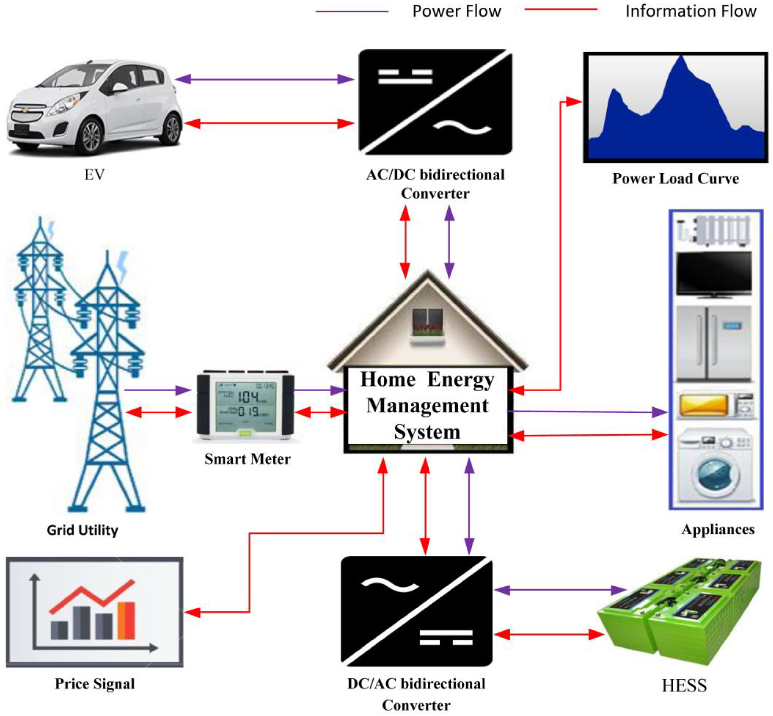
2.1. Smart Home Structure

Figure 1 illustrates the studied smart home diagram, which mainly consists of a set of household appliances, EV, HESS, the daily price signal, daily load curve, smart meter, grid utility, and HEMS to controls the energy flow between the HESS, EV, grid utility, and household appliances. Moreover, bi-directional DC/AC converters connect HESS and EV with grid utility and household appliances. A smart meter is necessary to gather data about the power amount needed or delivered to the utility grid in order to create an ideal energy scheduling between the power grid and the smart house under study, while smart home energy management system (HEMS) is also in charge of ensuring the best possible energy exchange between the components of smart homes and the utility grid. The phrase “smart home” in this study refers to a home that can offer two-way data connection and bidirectional power flow, which is consistent with the idea of a smart grid. HEMS receive TOU electricity price, the specific daily load curve, HESS parameters, and EV parameters as inputs to manage the energy scheduling among HESS, EV, smart home, and power grid based on several constraints such as: SOC of ESS and EV, charge and discharge of HESS and EV, charge, and discharge priority. The major contribution of this study is to control several operating modes for HESS and EV depending on the above constraints to ensure the power exchange between HESS, EV, and smart home, for the purpose of shaving peak load in the high-price periods and filling the valley in low price periods, thus smoothing daily load curve and reduce electricity cost in the smart home.

2.2. System Modeling

2.2.1. EV Modeling

As is well known, the spread of EVs plays an important role in home energy management thanks to energy exchange from grid-to-vehicle and V2H. Therefore, the concept of V2H is utilized to take advantage of the electric vehicle for reducing cost and flattening the load curve. The scheduling of the electric vehicle operation depends on its availability at home. The electric vehicle role should be accounted for depending on its availability at home, which is specified by the arrival ( t a ), and departure ( t d ) times. Being constrained by the capacity of the EV battery, the SOC of the EV battery will change dynamically due to charging from the grid utility or discharging to feed the demand by V2H. Therefore, the EV battery SOC estimation is an essential part of the HEMS, which will directly affect the decision and control of the home energy management system and the efficient use of the EV. The EV battery state of charge at a time interval (t) ( S O C E V t ) can be formulated based on the EV battery state of charge at the previous interval ( S O C E V t 1 ), as follows:
S O C E V t = S O C E V t 1 + η c E V P G E V t Q r a t e d E V i f c h   arg   i n g S O C E V t 1 P E V L t η d E V Q r a t e d E V i f d i s c h   arg   i n g , t a < t < t d
where P G E V t represents the power from the grid to vehicle (kW), P E V L t represents the power from the vehicle to load (kW), Q r a t e d E V is the rated capacity of the EV battery (kWh), η c E V is the EV battery charge efficiency, and η d E V is the EV battery discharge efficiency.
Due to the EV battery packs dynamic performance, the EV battery SOC is restricted in the range of allowed minimum ( S O C min E V ) and maximum ( S O C max E V ) values, as in Equations (2) and (3), respectively.
S O C E V t S O C min E V , t a < t < t d
S O C E V t S O C max E V , t a < t < t d
To provide the required energy for the electric vehicle trip distance, the EV battery state of charge at departure time should be greater than or equal to the required SOC for the EV trip distance ( S O C R E V ), which can be satisfied by Equation (4). In other words, before the involvement of EV in the V2H process, the energy amount stored in the EV battery will be verified to be enough for the remaining vehicle trip distance to ensure that the required energy for the EV trip distance is satisfied based on vehicle trip distance. The challenge in determining the required energy for EV at the departure time is primarily related to the dynamic nature of factors affecting energy consumption in the EV. Because the EV energy consumption is affected by several factors such as traffic, weather conditions, and vehicle performance, can all influence energy consumption even on the same routes. Therefore, regarding estimating the energy required for the distance of EV trip in this study, we took into account the average and worst-case scenarios to provide a reasonable estimate.
S O C E V t S O C R E V , t = t d
Finally, the EV battery state of charge at arrival time is calculated as in Equation (5).
S O C E V t = S O C E V t d S O C R E V , t = t a

2.2.2. HESS Modeling

Similar to EV battery, the HESS SOC will change dynamically due to charging from the grid utility or discharging to feed the demand. Moreover, the estimation of the HESS SOC will directly affect the decision and control of the HEMS and the efficient use of the HESS. Therefore, the HESS state of charge at a time interval (t) ( S O C B t ) can be modeled depending on the previous HESS state of charge ( S O C B t 1 ) as in Equation (6).
S O C B t = S O C B t 1 + η c B P G B t Q r a t e d B i f c h   arg   i n g S O C B t 1 P B L t η d B Q r a t e d B i f d i s c h   arg   i n g , t
where P G B t is the power from the grid-to-HESS (kW), P B L t is the power from the HESS-to-load (kW), Q r a t e d B is the rated capacity of the HESS (kWh), η c B is the HESS charge efficiency, and η d B is the HESS discharge efficiency.
Similar to the EV battery state of charge constraint, the HESS state of charge is also constrained between the minimum ( S O C min B ) and maximum ( S O C max B ) limits by using the constraints (5) and (6), respectively.
S O C B t S O C min B , t
S O C B t S O C max B , t

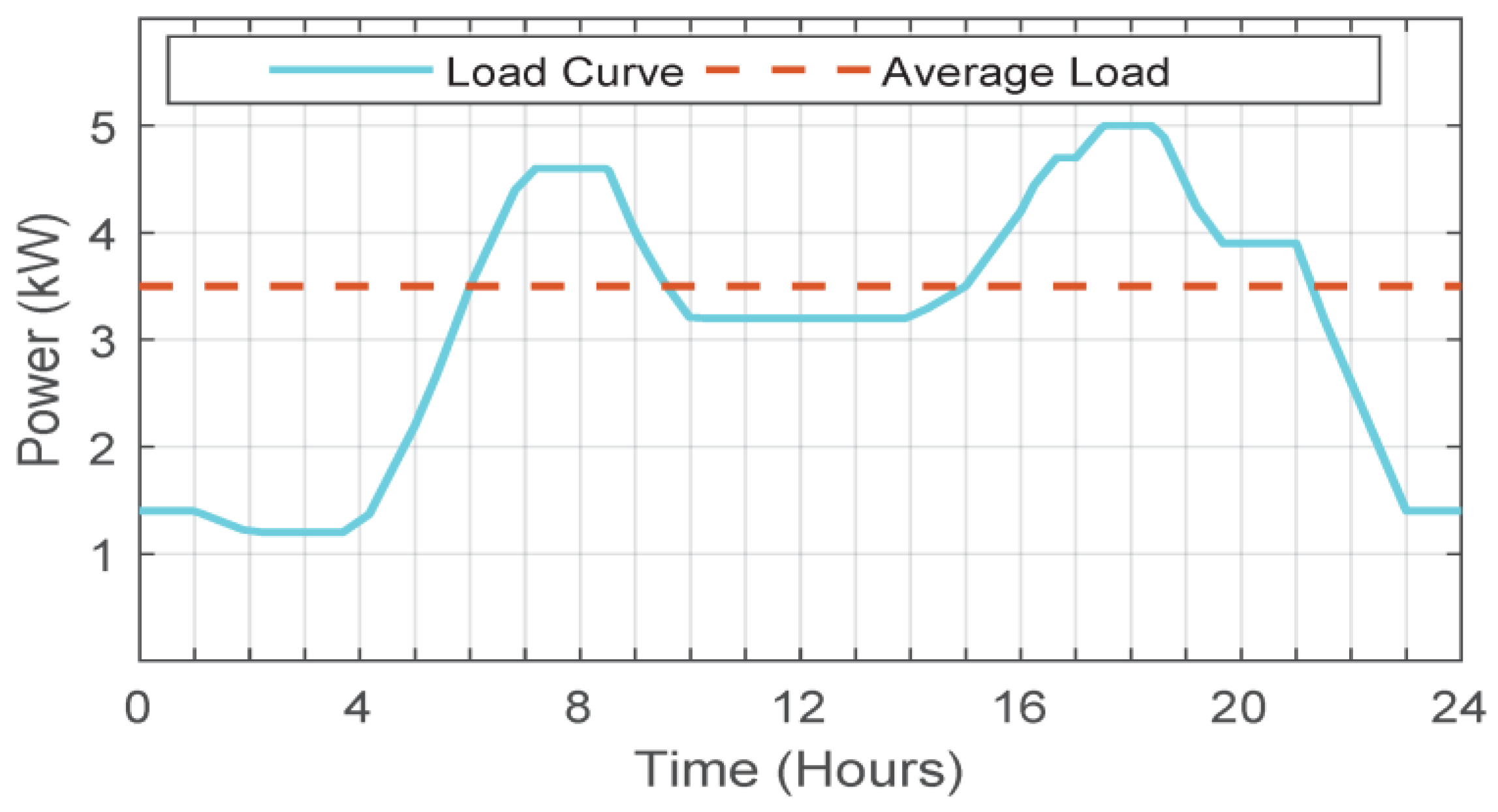
2.2.3. Daily Household Power Load

The smart home energy consumption by household appliances creates a curve known as the daily load curve. Therefore, the total energy consumed during the day can be found by the sum of all energy consumed by the household appliances throughout the day, which can be modeled as in Equation (9).
W D = t = 1 24 P L t
where W D is the total energy consumption of the household appliances throughout the day (kWh), and P L t is the energy consumption of the household appliances at time interval t (kW).
In this study, it is assumed that the smart home has contains EV. Therefore, the daily average energy consumption of the smart home is calculated by adding the average energy consumed by the household appliances throughout the day with EV average energy required for EV travel distance during the day, which can be formulated as in Equation (10).
P a v g = W D + E R E V 24
where P a v g is the daily average energy consumption by EV and household appliances (kW) and E R E V is the required energy for the EV travel distance in the typical day (kWh).
The required energy for the electric vehicle trip distance can be calculated by the following equation [34,35].
E R E V = η V D
where η V represents vehicle efficiency (kWh/km), and D represents the vehicle travel distance (km).

2.2.4. Daily Electricity Cost-Benefit Model

In this paper, one of the main objectives for the proposed energy management strategy in the studied home, illustrated in Figure 1, is to minimize total daily electricity costs while meeting the household energy demand and vehicle charging requirements. Reducing electricity costs is represented in charging the EV and/or household battery from the grid when the price of electricity is low (off-peak periods), in addition to discharging the HESS and/or EV to feed the load regardless of the electricity price. Therefore, the daily electricity cost reduction in the home under study is represented by the following equation:
min C D T = t = 1 24 λ t P L t P B L t P E V L t + t = 1 24 λ o f f t P G E V t + P G B t + C D B + C D E V
where C D T is the total daily energy consumption cost ($/day), λ t represents the price of electricity during different periods ($/kWh), λ o f f t represents the price of electricity during off-peak period ($/kWh), C D B represents daily capital cost for HESS installation ($/day), and C D E V represents daily EV battery degradation cost ($/day).
The daily electricity price during different periods can be formulated as.
λ t = λ o n t , t = t o n λ m i d t , t = t m i d λ o f f t , t = t o f f
where λ o n t is the electricity price during on-peak period ($/kWh), and λ m i d t is the electricity price during mid-peak period ($/kWh).
The daily capital cost for HESS installation, modeled as in Equation (14)
C D B = C B r 1 + r N 1 + r N 1 Q r a t e d B N d a y s
where C B represents the HESS one time installation cost ($/kWh), r represents the interest rate, N represents lifespan (years), and N d a y s represents the total number of days in the year.
The cost of EV battery degradation due to V2H can be calculated as follows.
C D E V = C E V C f D O D Q r a t e d E V D O D E R E V η d E V
where C E V represents EV battery replacement cost ($/kWh), C f represents the number of possible full cycles during a battery lifetime, and DOD represents depth of discharge of EV battery.

3. Proposed Energy Management Strategy (EMS)

The efficient scheduling of the charging and discharging of HESS and EV provided by the HEMS can significantly reduce load variation, electricity costs in smart homes and improve energy utilization. Therefore, this work presents a novel energy management strategy with different scenarios for reducing electricity bills and smoothing the load curve in the smart house that contains EV with/without HESS. In this work energy usage is optimized based on the flowcharts presented in Figure 2, Figure 3, Figure 4 and Figure 5. The proposed energy management strategy operates in different modes to control the energy amount flowing from the grid to the EV and/or HESS and the energy amount drawn from the EV and/or HESS to feeding the load, in addition to detect the suitable time to charge and discharge the EV and HESS. To reduce the load variation and electricity bill in the smart home that contains EV with/without HESS, the charging/discharging schedule scenarios for EV and/or HESS must meet the following prohibitions (Table 1):

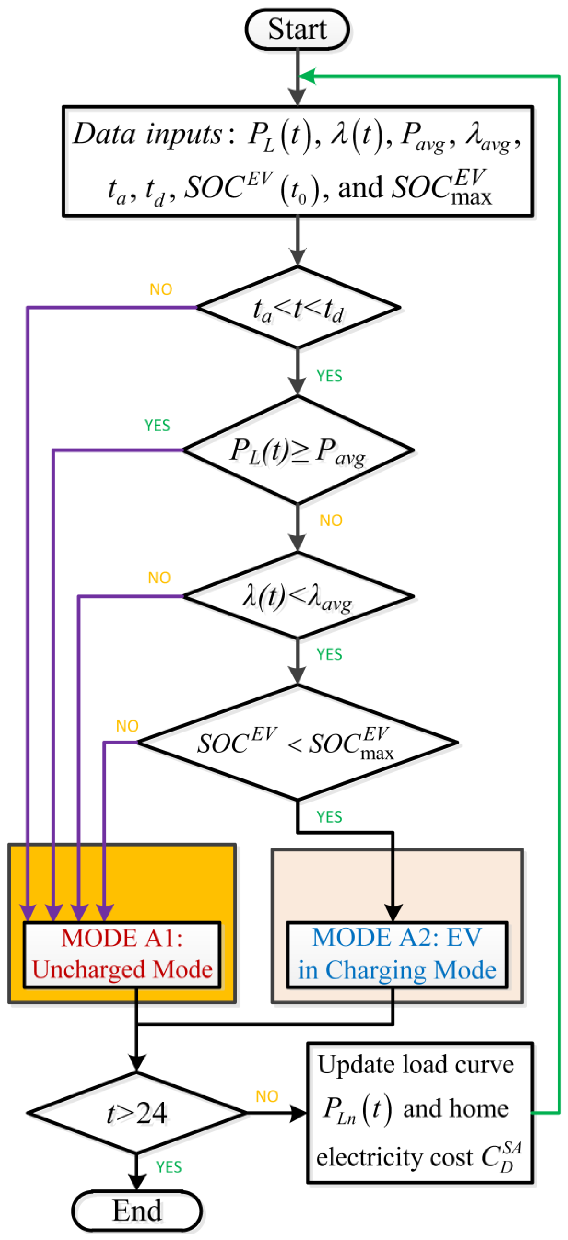
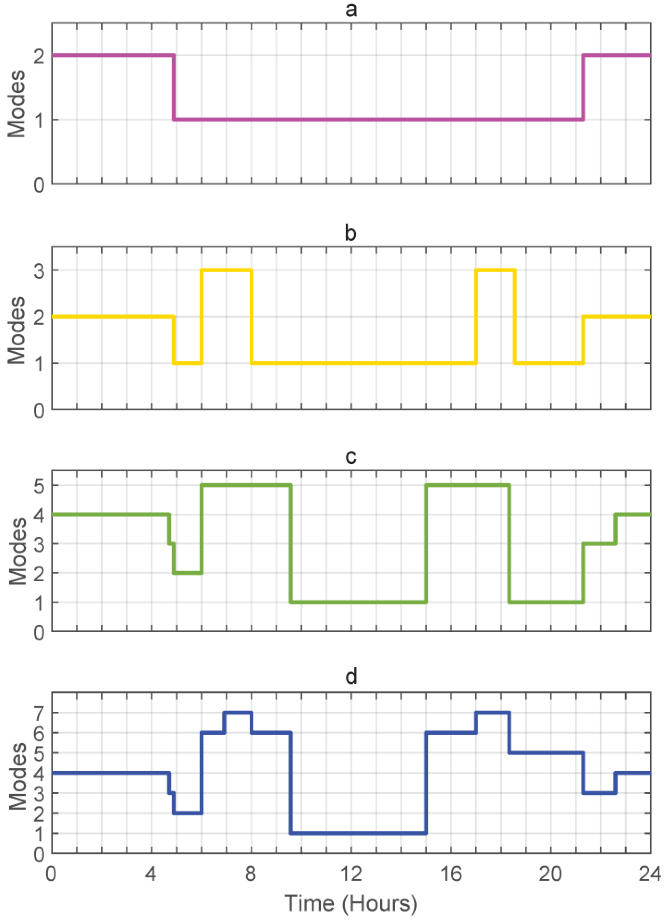
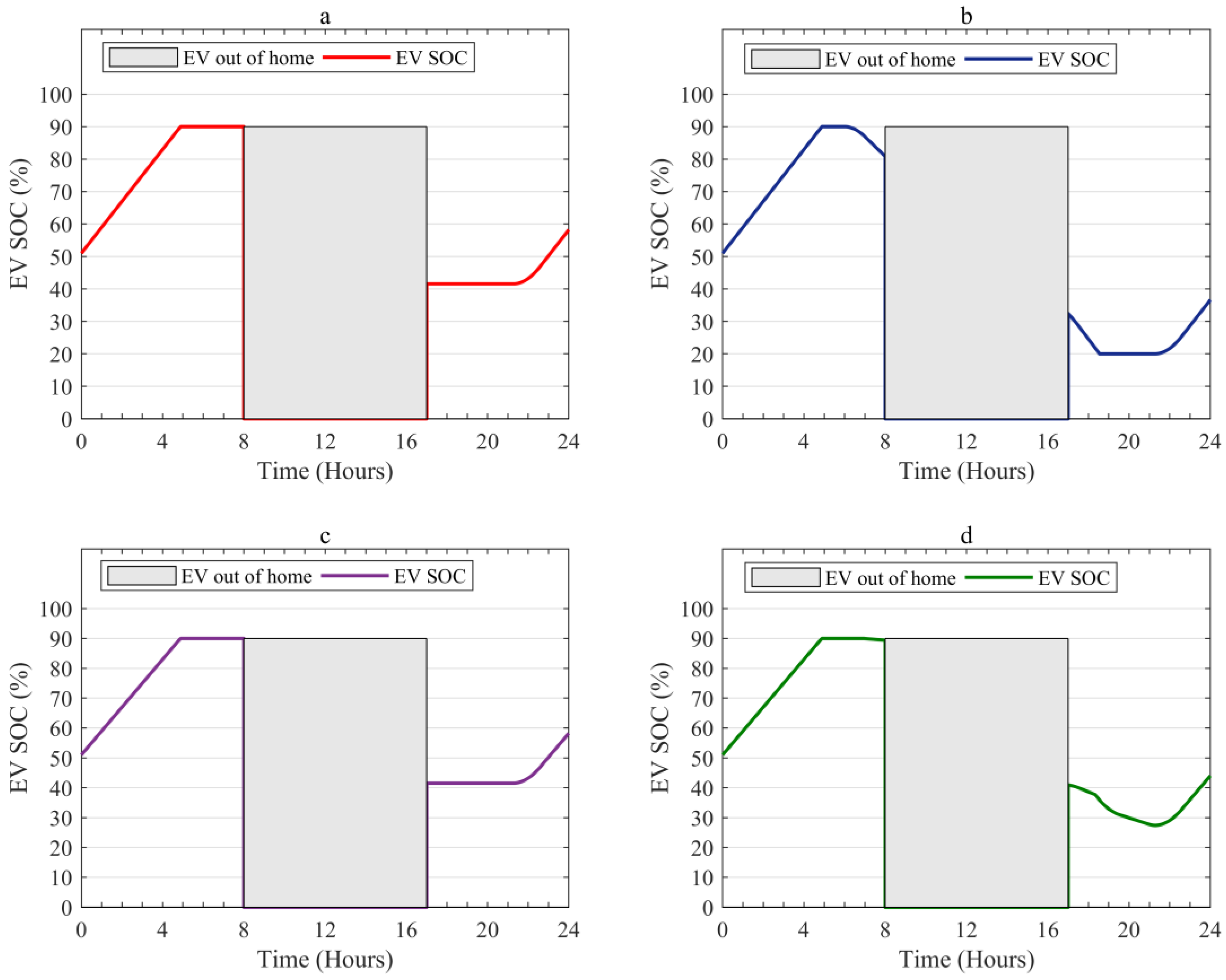
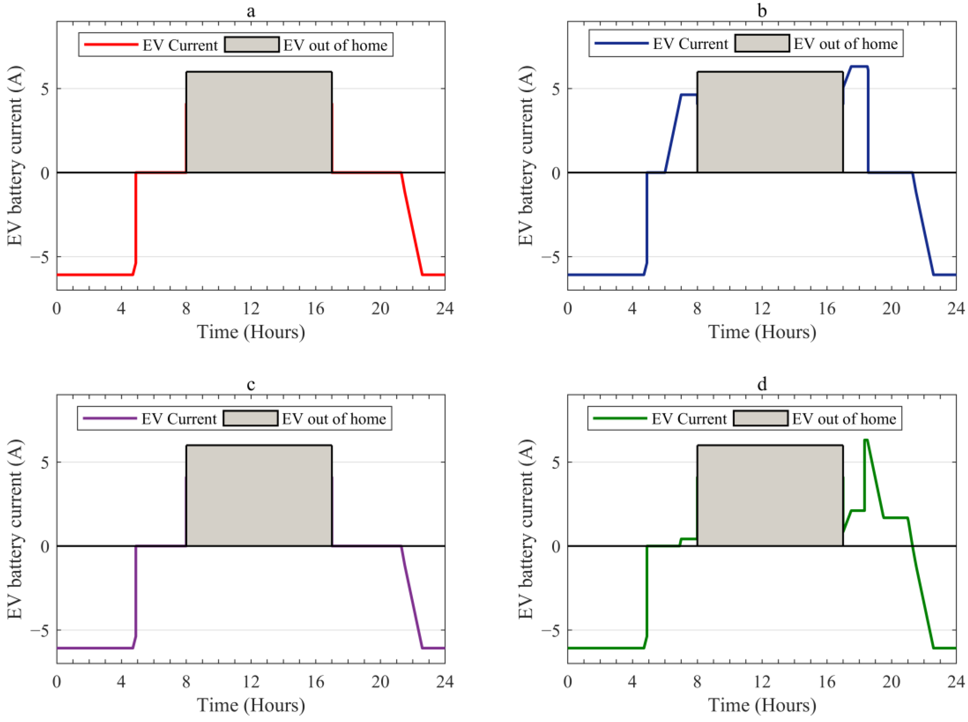
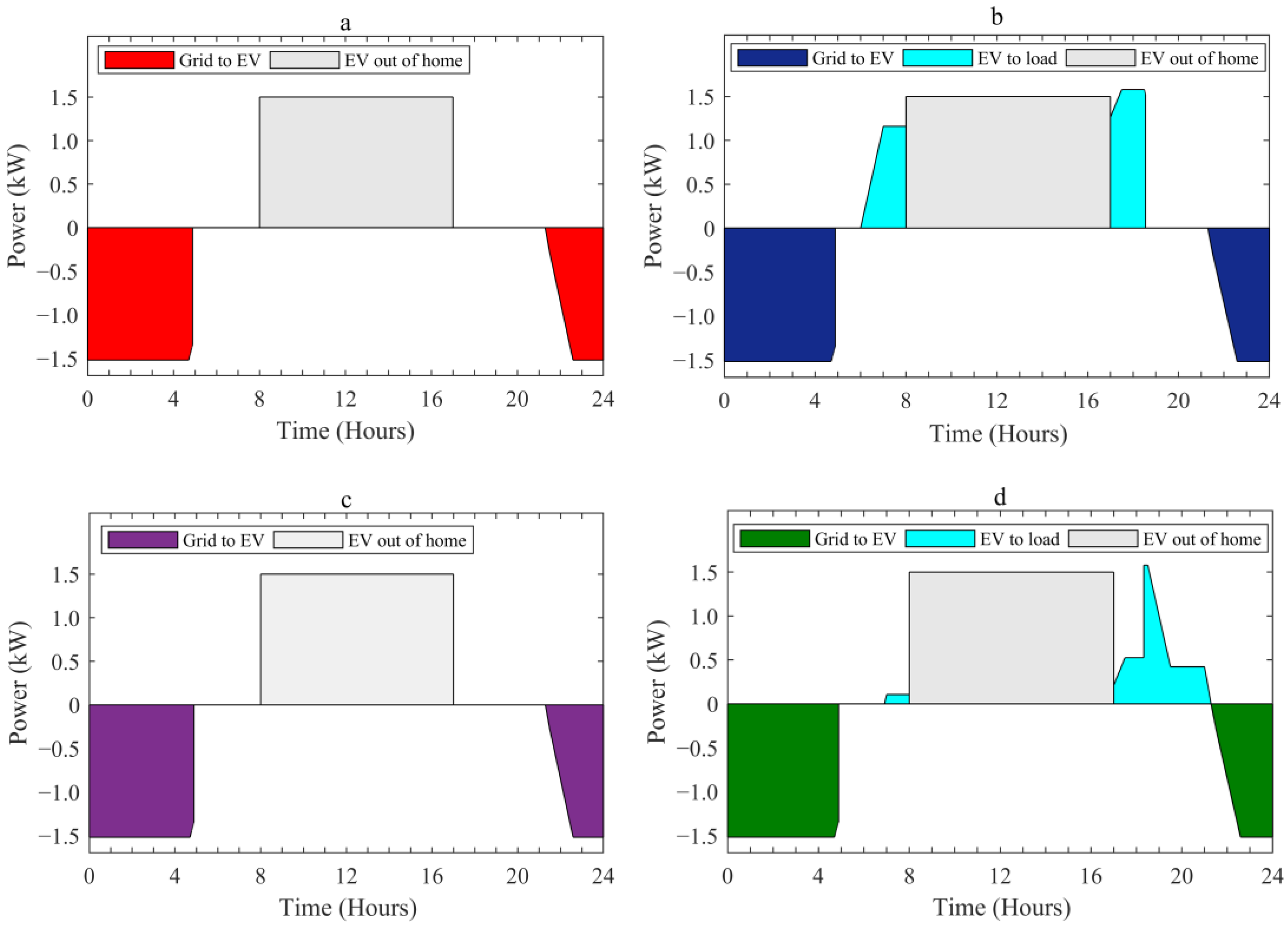
3.1. Scenario A: Control EV Charging without V2H and HESS

3.1.1. Energy Scheduling of EV Charging without V2H and HESS

In this scenario, the electric vehicle is considered as an electrical load only. However, the EV will be charged in a controlled regime depending on the electricity price curve and the power load curve. The control algorithm shown in Figure 2 receives, the daily household appliances load profile P L t , electricity price signal λ t , average load P a v g , average electricity price λ a v g , arrival and departure times of EV t a and t d , initial SOC of the EV battery S O C E V t 0 , and maximum SOC of the EV battery S O C max E V , as inputs. Thus, the control algorithm will control the household energy in two modes as follows:
  • MODE A1: Uncharged Mode
In this mode, the electric vehicle battery is not charged. This mode is achieved by activation one of these four statuses: (i) the electric vehicle is out of the house; (ii) the EV is at the house and P L t is equal or higher than P a v g ; (iii) the EV is at the house and the P L t is less than P a v g , but λ t is equal or higher than λ a v g ; (v) EV is at the house, the P L t is less than P a v g , and λ t is less than λ a v g , but the EV battery is equal or greater than S O C max E V . So, the household load demand will not change as in Equation (16).
P L n t = P L t
where P L n t is the new household power load curve (kW).
  • MODE A2: EV in Charging Mode
In this mode, EV is always in the charging mode. This mode is selected if the EV is at the house, the P L t is less than P a v g , λ t is less than λ a v g , and the EV battery $SOC$ is less than S O C max E V . Therefore, the EV charging in this mode is modeled by Equation (17), while the changing power load demand is expressed by Equation (19).
P G E V t = ( P L t P a v g )
P L n t = P L t + P G E V t

3.1.2. Cost Reduction in EV Charging without V2H and HESS

In this scenario, the total electricity cost is affected by Equation (17), which describes the amount of energy that EV consumes when the price and consumption of electricity are low. Since the home without V2H and HESS, the part related to V2H and HESS in Equation (12) becomes zero. Therefore, Equation (12) is reformulated as follows.
min C D T , S A = t = 1 24 λ t P L t + t = 1 24 λ o f f t P G E V t
where C D T , S A is the total daily energy consumption cost in scenario A ($/day).

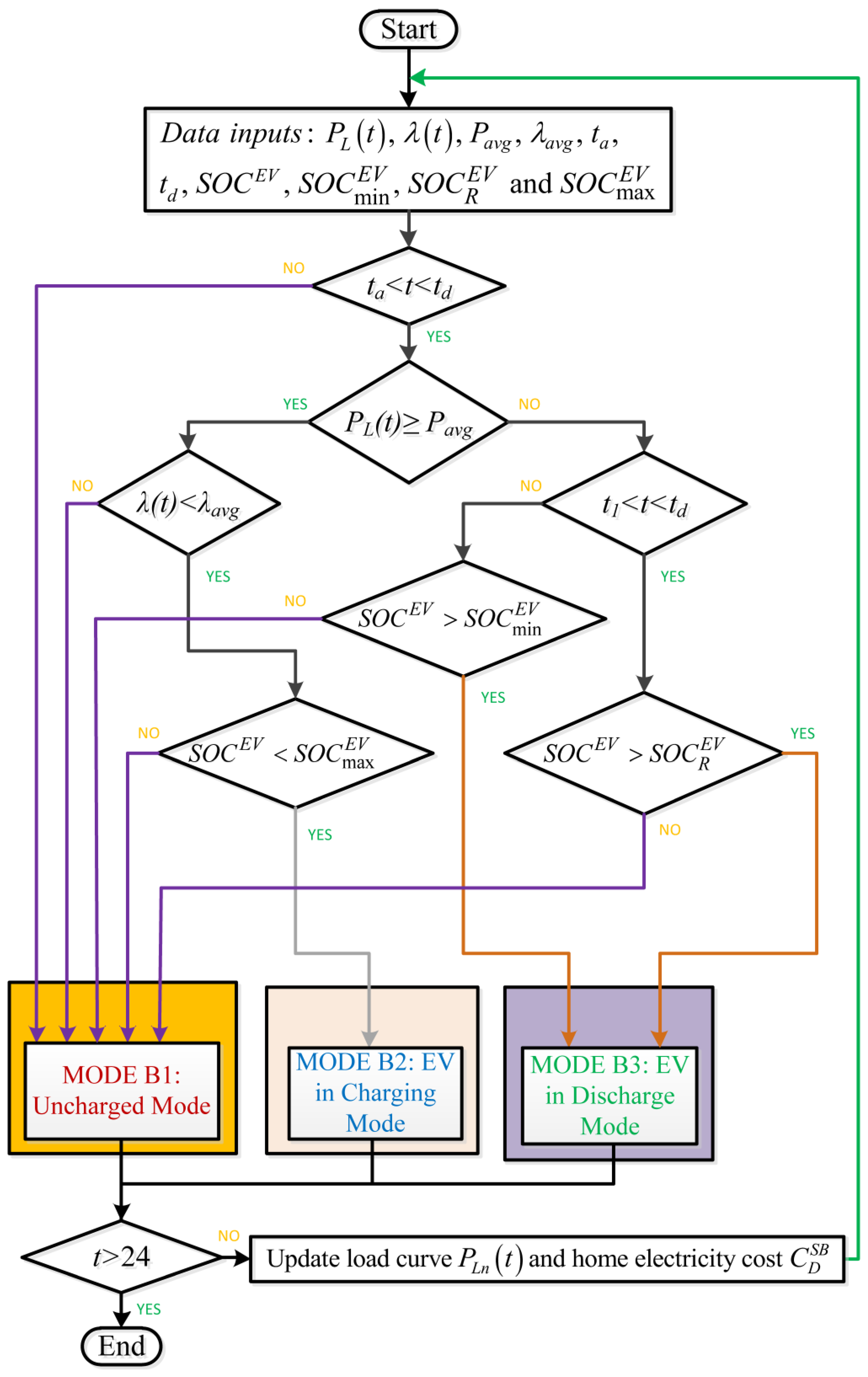
3.2. Scenario B: Control EV Charging with V2H without HESS

3.2.1. Energy Scheduling of EV Charging with V2H without HESS

In this scenario, the electric vehicle is charged and discharged in a controlled regime depending on the electricity price curve and the power load curve. The electric vehicle is used as energy storage, which is charged if the consumption and price of electricity are low and discharged to feed the load demand at peak time by V2H. The control algorithm shown in Figure 3 receives, P L t , λ t , P a v g , λ a v g , t a , t d , S O C E V t 0 , S O C max E V , minimum state of charge of the EV battery S O C min E V , and required SOC for the EV trip distance S O C R E V as inputs. After that, the control algorithm will control the household energy by the following three modes:
  • MODE B1: Uncharged Mode
The electric vehicle battery will not charge or discharge in this mode. This mode is achieved by operating one of these five statuses: (i) the electric vehicle is out of the house; (ii) the EV is at home and the P L t is less than P a v g , but λ t is equal or higher than λ a v g ; (iii) EV is at the house, the P L t is less than P a v g , and λ t is less than λ a v g , but the EV battery SOC is equal to S O C max E V ; (iv) the electric vehicle is at the house, the P L t is equal or higher than P a v g , and time was between arrival time and midnight t a < t < t 24 , but the EV battery SOC is equal to S O C min E V ; (v) the electric vehicle is at the house, the P L t is equal or higher than P a v g , and time was between midnight and departure time t 00 < t < t d but the EV battery SOC is equal to S O C R E V . Therefore, the household load demand will not change as in Equation (16).
  • MODE B2: EV in Charging Mode
In this mode, the EV is always in the charging mode. This mode is selected when the EV is at house, the P L t is less than P a v g , the λ t is less than λ a v g , time was between arrival time and midnight, and the EV battery SOC is less than S O C max E V . Therefore, the EV charging in this mode is modeled by Equation (17), while changing power load demand is expressed by Equation (18).
  • MODE B3: EV in discharging Mode
In this mode, EV is always in the discharging mode. This mode is achieved by tow statuses: (i) the EV is at the house, the P L t is equal or higher than P a v g , time was between arrival time and midnight t a < t < t 24 and the EV battery SOC is greater than S O C min E V ; (ii) the EV is at the house, the P L t is equal or higher than P a v g , time was between midnight and departure time t 00 < t < t d and the EV battery SOC is greater than S O C R E V . Therefore, in this mode, electric vehicle is discharging to feeding the load as in Equation (20), and the household load demand will change as modeled as in Equation (21).
P E V L t = P L t P a v g
P L n t = P L t P E V L t

3.2.2. Cost Reduction in EV Charging with V2H without HESS

In this scenario, the total electricity cost is affected by Equation (17), and Equation (20) which describes the amount of power that EV consumes if the consumption and price of electricity are low, and the quantity of power injected to the load from electric vehicle at peak time, respectively. Being the home without HESS, the part related to HESS in Equation (12) becomes zero. Therefore, Equation (12) is rewritten as follows.
min C D T , S B = t = 1 24 λ t [ P L t P E V L t ] + t = 1 24 λ o f f t P G E V t + C D E V
where C D T , S B represents the total daily energy consumption cost in scenario B ($/day).

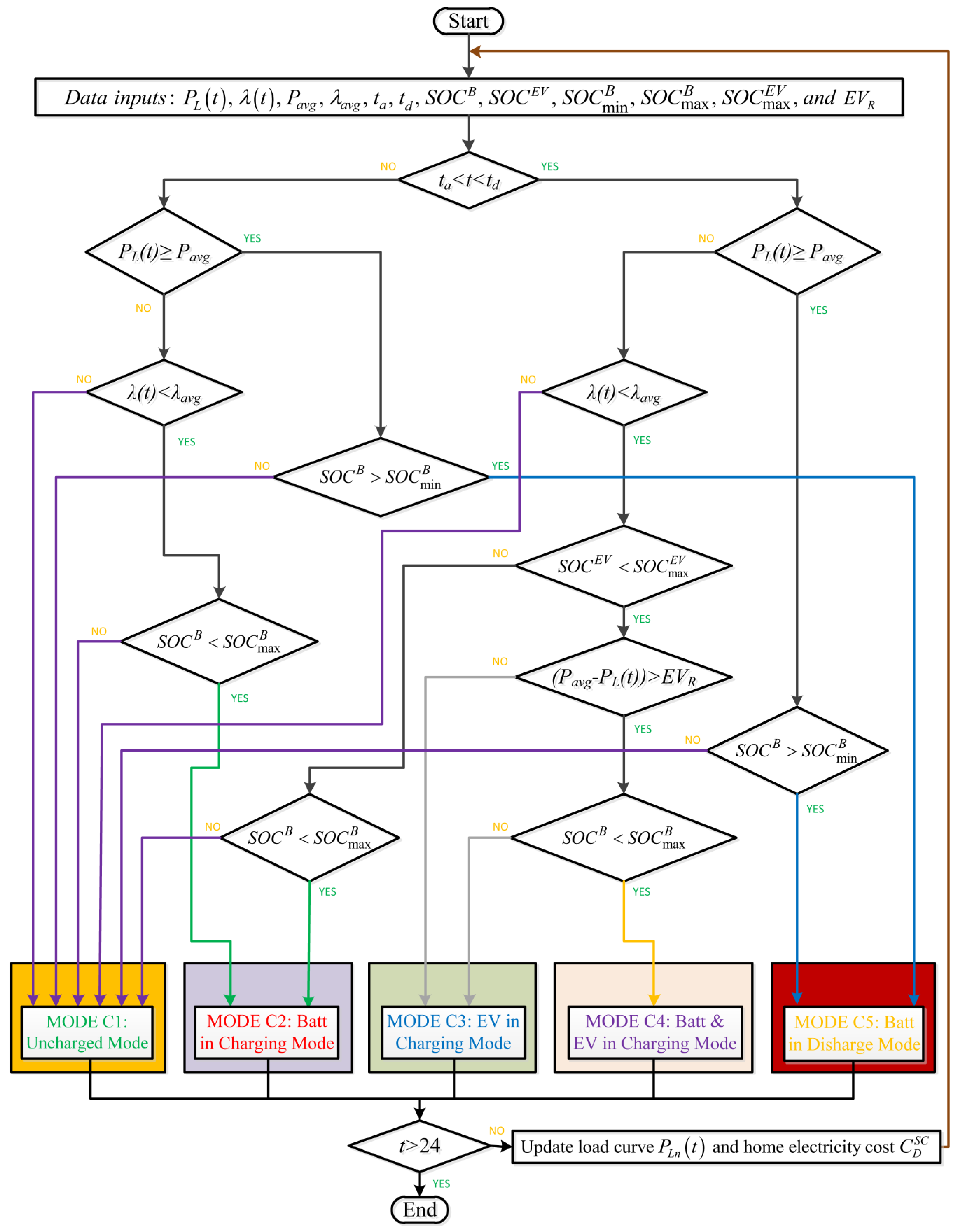
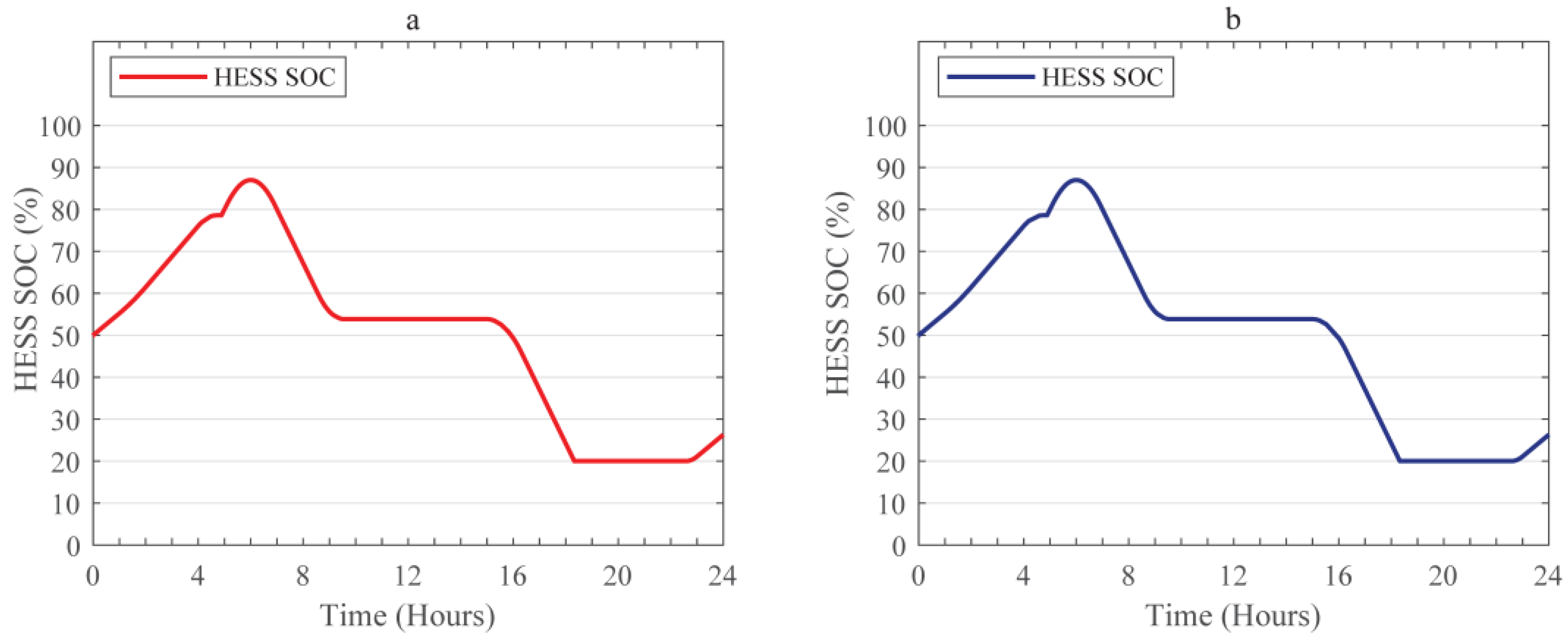
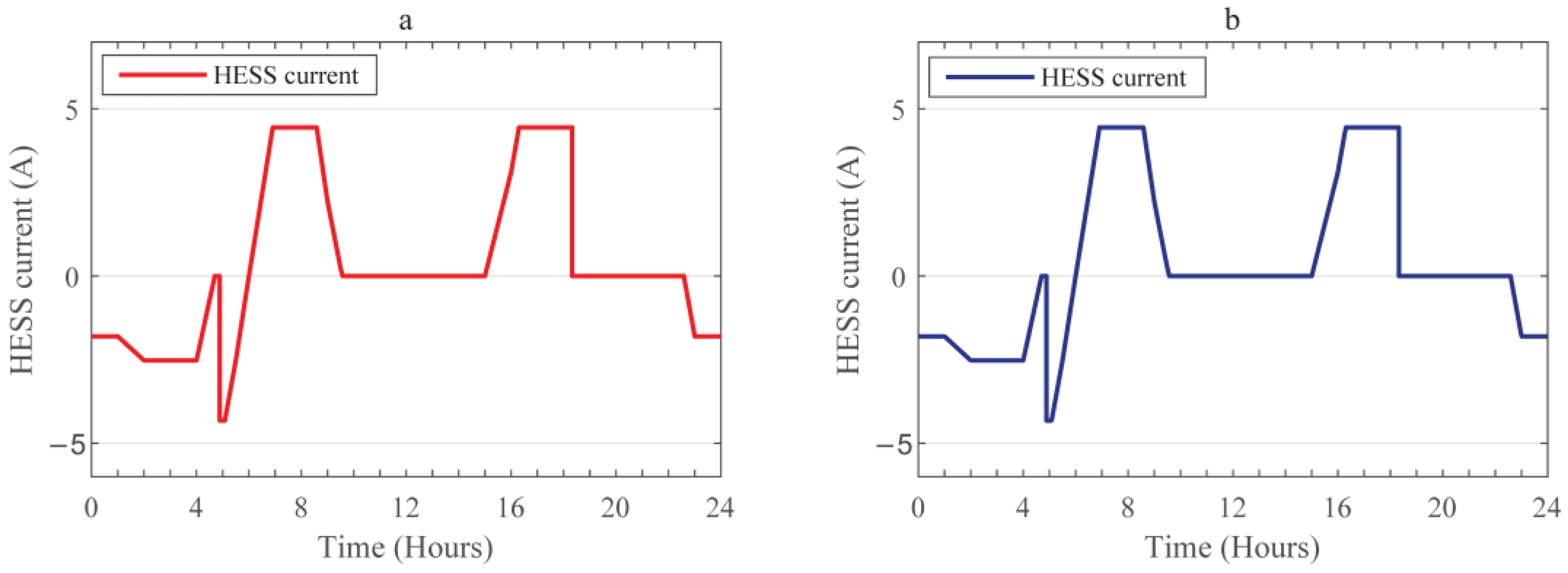
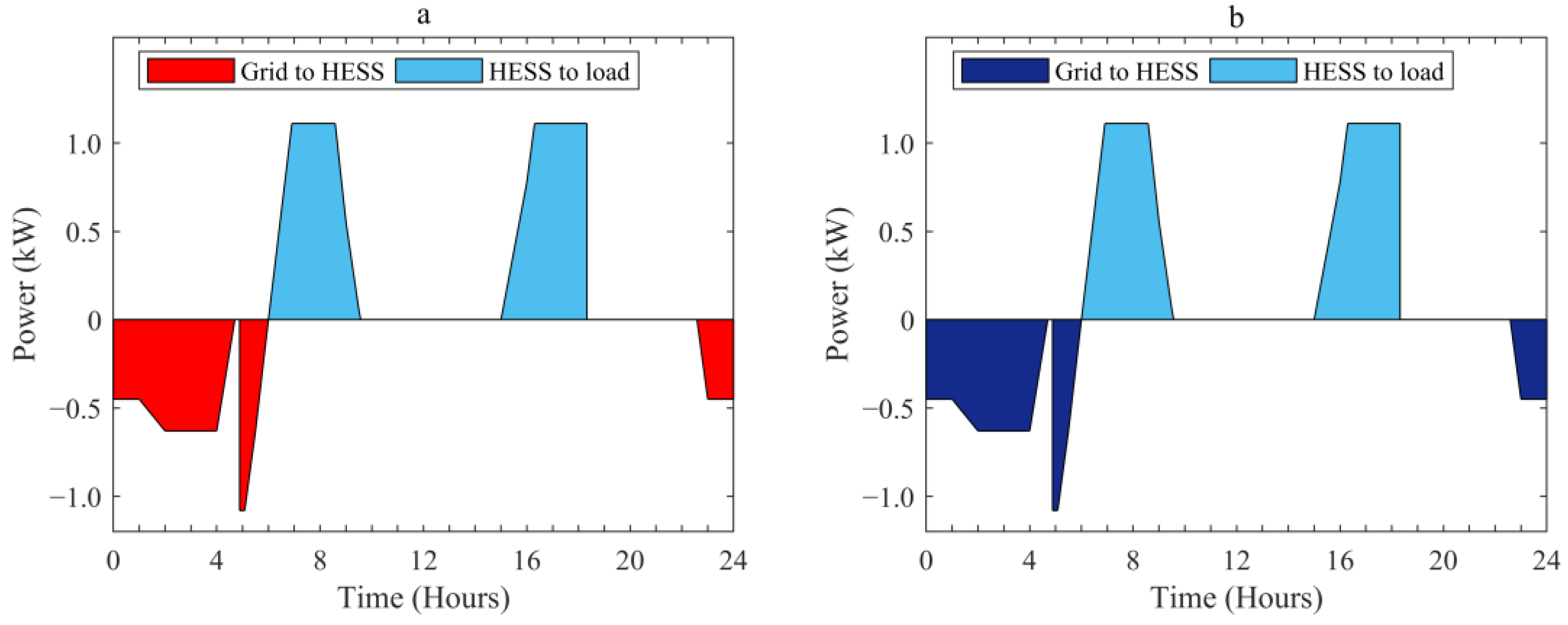
3.3. Scenario C: Control EV Charging with HESS without V2H

3.3.1. Energy Scheduling of EV Charging with HESS without V2H

In this scenario, the EV is charged, and HESS is charged/discharged in a controlled regime depending on the electricity price curve and the power load curve. The EV is used as a load, and it will charge if the consumption and price of electricity are low. In contrast, HESS is utilized as an electrical load when the price and consumption of electricity are low, and it will be utilized as a supply to feed the demand at peak time. The control algorithm shown in Figure 4 receives, the P L t , λ t , P a v g , λ a v g , t a , t d , S O C E V t 0 , S O C max E V , the initial state of charge of the HESS S O C B t 0 , minimum state of charge of the HESS S O C min B , maximum state of charge of the HESS S O C max B , and rated charge power of EV E V R as inputs. Then, the control algorithm will control the household energy in five modes as follows:
  • MODE C1: Uncharged Mode
In this mode, the electric vehicle battery is not charged, and HESS will not be charged or discharged. This mode is achieved by one of these six statuses: (i) the electric vehicle is out of the house, the P L t is less than P a v g , and λ t is equal or higher than λ a v g ; (ii) the EV is out of the house, the P L t is equal or higher than P a v g , and the HESS S O C B is equal to S O C min B ; (iii) the EV is out of the house, the P L t is less than P a v g , λ t is less than λ a v g , and the HESS S O C B is equal to S O C max B ; (iv) the EV is at the house, the P L t is less than P a v g , and λ t is equal or higher than λ a v g ; (v) EV is at the house, the P L t is equal or higher than P a v g , and the HESS S O C B is equal to S O C min B ; or (vi) the EV is at the house, the P L t is less than P a v g , λ t is less than λ a v g , the EV S O C E V is equal to S O C max E V , and the HESS S O C B is equal to S O C max B . Therefore, the household load demand will not change, as in Equation (16).
  • MODE C2: HESS in Charging Mode
In this mode, HESS only in the charging mode. This mode is selected through two statuses: (i) the EV is out of the house, the P L t is less than P a v g , λ t is less than λ a v g , and the HESS S O C B is less than S O C max B ; or (ii) the EV is at home, the P L t is less than P a v g , λ t is less than λ a v g , the EV S O C E V is equal to S O C max E V , and the HESS S O C B is less than S O C max B . Therefore, HESS charged from the grid can be modeled as in Equation (23), and the household load demand will change by Equation (24).
P G B t = ( P L t P a v g )
P L n t = P L t + P G B t
  • MODE C3: EV in Charging Mode
In this mode, EV only in the charging mode. This mode is selected through two statuses: (i) the EV is at the house, the P L t is less than P a v g , λ t is less than λ a v g , the EV S O C E V is less than S O C max E V , and ( P a v g P L t ) is equal or less than EV rated charge power E V R ; or (ii) the EV is at the house, the P L t is less than P a v g , λ t is less than λ a v g , the EV S O C E V is less than S O C max E V , and ( P a v g P L t ) greater than EV rated charge power E V R , but the HESS S O C B is equal S O C max B . Therefore, the EV charging in this mode is modeled by Equation (17), while the changing power load demand is expressed by Equation (18).
  • MODE C4: EV and HESS in Charging Mode
This mode is activated when the electric vehicle is at the house, the P L t is less than P a v g , λ t is less than λ a v g , the EV battery S O C E V is less than S O C max E V , ( P a v g P L t ) is greater than EV rated charge power E V R , and HESS S O C B is less than S O C max B . In this mode, EV and HESS are in charging mode, thus the energy flow from grid-to-vehicle, grid-to-HESS, and changed household load are modeled as in Equations (25)–(27), respectively.
P G E V t = E V R
P G B t = ( P L t P a v g ) E V R
P L n t = P L t + P G E V t + P G B t
  • MODE C5: HESS in Discharging Mode
The HESS is discharged to feeding the load in this mode. This mode is activated through two statuses: (i) the electric vehicle is at the house, the P L t is equal or greater than P a v g , and the HESS S O C B is greater than S O C min B ; or (ii) the EV is out of the house, the P L t is equal or greater than P a v g , HESS S O C B is greater than S O C min B . Therefore, the HESS discharge in this mode is modeled by Equation (28), while the changing power load is modeled by Equation (29).
P B L t = P L t P a v g
P L n t = P L t P B L t

3.3.2. Cost Reduction in EV Charging with HESS without V2H

In this scenario, the total electricity cost is affected by charging EV through Equations (17) and (25), if the consumption and price of electricity are low, and by charging HESS through Equation (23) and Equation (26), also when the price and consumption of electricity are low. In addition, HESS discharge to feed the load at peak time is calculated through Equation (28). Since the home without V2H, the part related to V2H in Equation (12) becomes zero. Therefore, Equation (12) is rewritten as follows.
min C D T , S C = t = 1 24 λ t P L t P B L t + t = 1 24 λ o f f t P G E V t + P G B t + C D B
where C D T , S C is the total daily energy consumption cost in scenario C ($/day).

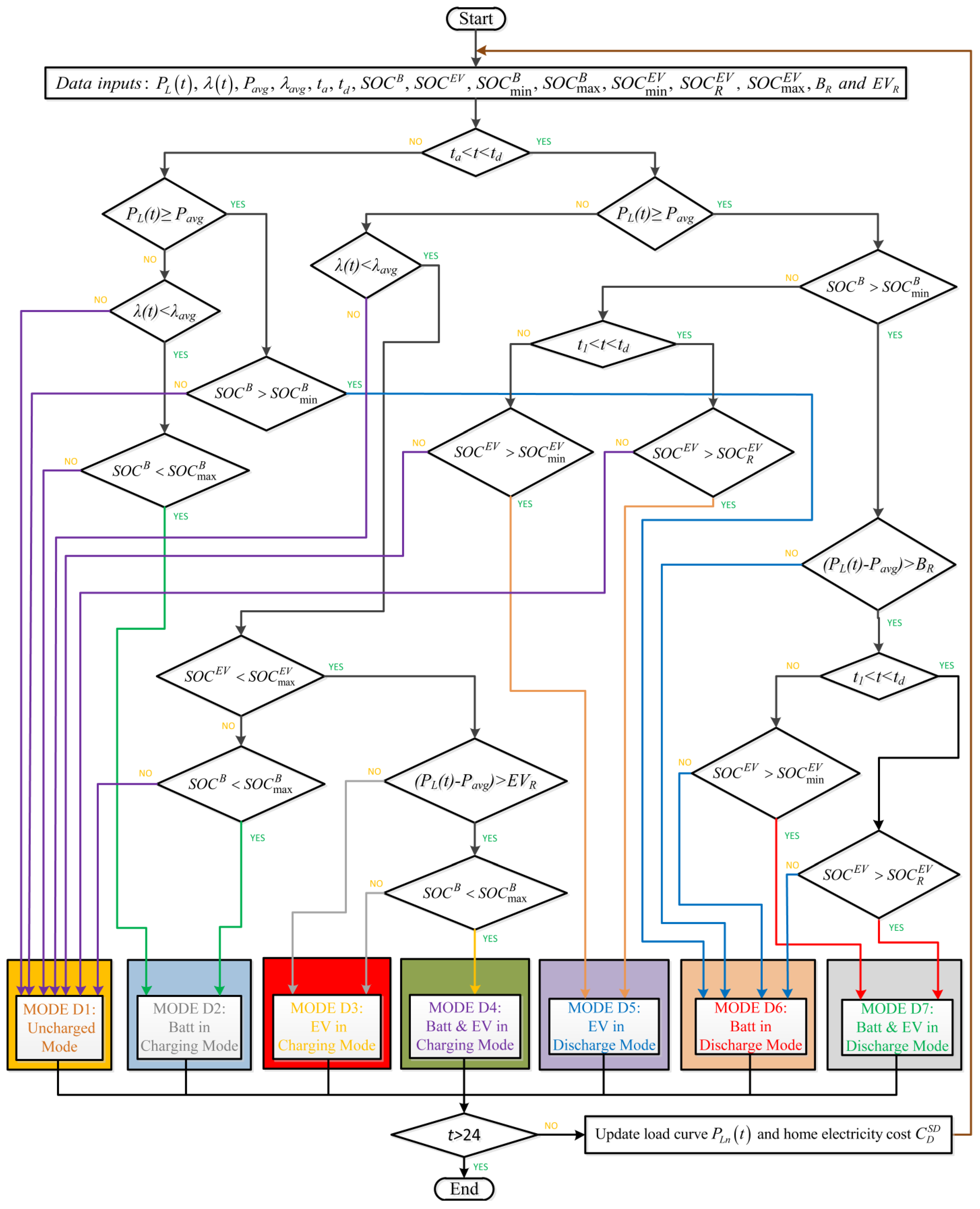
3.4. Scenario D: Control EV Charging with V2H and HESS

3.4.1. Energy Scheduling of EV Charging with V2H and HESS

In this scenario, the electric vehicle and HESS are charging/discharging in a controlled regime depending on the electricity price curve and the power load curve. The electric vehicle and HESS are utilized as energy storage, charged when the prices and consumption of electricity are low, and discharged to feed the load demand during peak hours. The control algorithm shown in Figure 5 receives, the P L t , λ t , P a v g , λ a v g , t a , t d , S O C B t , S O C E V t , S O C min B , S O C max B , S O C min E V , S O C max E V , S O C R E V , E V R , and rated discharge power of HESS B R , as inputs. Thus, the control algorithm will control the household energy in seven modes as follows:
  • MODE D1: Unchanged Mode
The electric vehicle and HESS will not charge or discharge in this mode. This mode is selected by one of these seven statuses: (i) the electric vehicle is out of the house, the P L t is less than P a v g , and λ t is equal or higher than λ a v g ; (ii) the EV is out of the hose, the P L t is equal or higher than P a v g , and the HESS S O C B is equal to S O C min B ; (iii) the EV is out of the house, the P L t is less than P a v g , λ t is less than λ a v g , and the HESS S O C B is equal to S O C max B ; (iv) the EV is at the house, P L t is less than P a v g , and λ t is equal or higher than λ a v g ; (v) the EV is at the house, the P L t was less than P a v g , λ t is less than λ a v g , the EV S O C E V is equal to S O C max E V , and HESS S O C B is equal to S O C max B ; (vi) the EV is at the house, the P L t is equal or higher than P a v g , the HESS S O C B is equal to S O C min B , time was between arrival time and midnight t a < t < t 24 , and the EV battery S O C E V is equal to S O C max E V ; or (vii) the EV is at the house, the P L t is equal or higher than P a v g , the HESS S O C B is equal to S O C min B , time was between midnight and departure time t 00 < t < t d , and the EV battery S O C E V is equal to S O C R E V . Therefore, the household load demand will not change as in Equation (16).
  • MODE D2: HESS in Charging Mode
In this mode, HESS only in the charging mode. This mode is activated through two cases: (i) the EV is out of the house, the P L t is less than P a v g , λ t is less than λ a v g , and the HESS S O C B is less than S O C max B ; or (ii) the EV is at home, the P L t is less than P a v g , λ t is less than λ a v g , the EV S O C E V is equal to S O C max E V , and HESS S O C B is less than S O C max B . Therefore, HESS charged from the grid can be represented by Equation (23), and the changing household load demand can be modeled by Equation (24).
  • MODE D3: EV in Charging Mode
In this mode, EV only in the charging mode. This mode is selected through two statuses: (i) the EV is at the house, the P L t is less than P a v g , λ t is less than λ a v g , the EV S O C E V is less than S O C min E V , and ( P a v g P L t ) is less than or equal to E V R ; or (ii) the EV is at the house, the P L t is less than P a v g , λ t is less than λ a v g , the EV S O C E V is less than S O C max E V , and ( P a v g P L t ) greater than E V R , but the HESS S O C B is equal to S O C max B . Therefore, the EV charging in this mode is modeled by Equation (17), while the changing power load demand is expressed by Equation (18).
  • MODE D4: EV and HESS in Charging Mode
This mode is activated when the electric vehicle is at the house, P L t is less than P a v g , λ t is less than λ a v g , the EV battery S O C E V is less than S O C max E V , ( P a v g P L t ) is greater than E V R , and the HESS S O C B is less than S O C max B . In this mode, the EV and HESS are in charging mode, thus the energy flow from grid-to-vehicle, grid-to-HESS, and changed household load demand are modeled as in Equations (25), (26), and (27), respectively.
  • MODE D5: EV in Discharging Mode
In this mode, the electric vehicle is discharging to feeding the load. This mode is activated by one of these two statues: (i) the EV is at the house, the P L t is equal or higher than P a v g , the HESS S O C B is equal to S O C min B , time was between arrival time and midnight t a < t < t 24 , and the EV battery S O C E V is greater than S O C max E V ; or (ii) the EV is at the house, the P L t is equal or higher than P a v g , the HESS S O C B is equal to S O C min B , time was between midnight and departure time t 00 < t < t d , and the EV battery S O C E V is greater than S O C R E V . Therefore, the EV battery discharge in this mode is modeled by Equation (20), while the changing power load demand is expressed as in Equation (21).
  • MODE D6: HESS in Discharging Mode
In this mode, HESS is discharging to feeding the load. This mode is selected by one of these four statuses: (i) the electric vehicle is out of the house, the P L t is equal or higher than P a v g , HESS S O C B is greater than S O C min B ; (ii) the EV is at home, the P L t is equal or higher than P a v g , and the HESS S O C B is greater than S O C min B , and ( P L t P a v g ) is less than or equal to HESS rated discharge power B R ; (iii) the EV is at the house, the P L t is equal or higher than P a v g , the HESS SOC is greater than S O C min B , ( P L t P a v g ) is greater than HESS rated discharge power B R , time was between arrival time and midnight t a < t < t 24 , and the EV SOC is equal to S O C min E V ; or (iv) the EV is at the house, the P L t is equal or higher than P a v g , the HESS SOC is greater than S O C min B , ( P L t P a v g ) is greater than HESS rated discharge power B R , time was between midnight and departure time t 00 < t < t d , and the EV SOC is equal to S O C R E V . Therefore, the HESS discharge in this mode is expressed as in Equation (28), while the changing load demand is modeled by Equation (29).
  • MODE D7: HESS and EV in Discharging Mode
In this mode, the HESS and electric vehicle are discharging to feeding the demand, and it will activated by one of these two statuses: (i) the EV is a t the house, the P L t is equal or higher than P a v g , the HESS SOC is greater than S O C min B , ( P L t P a v g ) is greater than HESS rated discharge power B R , time was between arrival time and midnight t a < t < t 24 , and the EV SOC is greater than S O C min E V ; or (ii) the EV is at the house, the P L t is equal or higher than P a v g , the HESS SOC is greater than S O C min B , ( P L t P a v g ) is greater than HESS rated discharge power B R , time was between midnight and departure time t 00 < t < t d , and the EV SOC is greater than S O C R E V . The HESS discharging, EV discharging, and changed household demand are modeled by Equations (31), (32), and (33), respectively.
P B L t = B R
P E V L t = ( P L t P a v g ) B R
P L n t = P L t ( P B L t + P E V L t )

3.4.2. Cost Reduction in EV Charging with V2H and HESS

In this scenario, the total electricity cost is affected by charging EV through Equations (17) and (25), if the consumption and price of electricity are low, and by charging HESS through Equation (23), Equation (26), also when the price and consumption of electricity are low. In addition to EV discharge to feed load at peak hours through Equations (20) and (32) and HESS discharge to feed load at peak time through Equations (28) and (31). Therefore, in scenario D Equation (12) will not change, because it includes the part related to V2H and HESS and will be written as follows.
min C D T , S D = t = 1 24 λ t P L t P B L t P E V L t + t = 1 24 λ o f f t P G E V t + P G B t + C D B + C D E V
where C D T , S D represents the total daily energy consumption cost in scenario D ($/day).

4. Results and Discussion

This section analyzes the characteristics of the proposed energy management strategy with different scenarios. It compares their performance with the uncontrolled charging system in terms of load curve flattening and cost reduction to verify the effectiveness of the proposed energy management strategy. For simplicity, the simulation was executed within 24 h divided into 48 time intervals with a length of 30 min.
The time-varying price signals of electricity are taken from [36], which is based on Southern California Edison residential TOU rates. Table 2 shows residential electricity prices in on-peak hours, mid-peak hours, and off-peak hours provided by Southern California Edison. Moreover, Figure 6 depicts the time-varying electricity price curve that ranges between 0.12995–0.40824 $/kWh, with the average electricity price of 0.26018 $/kWh, which was taken to be equal to the mid-peak price in this paper. Thus, motivates a household to charge their EV and household battery in the off-peak hours (cheap electricity price) to take advantage of them at peak hours.
Near-real-time hourly electricity consumption data were collected from 48 states by the United States energy information administration. They found that household electricity consumption is low during the night and high in the evening and morning [37]. Therefore, in this work, the household appliances are predicted to consume low electricity during the night and high during evening and morning as depicted in Figure 7.
The EV and HESS parameters used in this simulation are listed in Table 3. In this work, the EV is charged and discharged with 1.5 kW, due to the adequate level to charge the EV in the house ranges between 1.5–3 kW [38]. The electric vehicle daily travel distance is considered 40 miles, which is the average travel distance in the United States [39].
Furthermore, it is assumed that the electric vehicle departed and arrived at the house at 08:00 and 17:00, respectively. The economical parameters of the battery and EV battery utilized in this paper are introduced in Table 4. The interest rate is considered to be 6%.
Figure 8 illustrates the transitions between different modes during the day for the four developed scenarios.
Figure 8a shows two different modes for the first scenario A, during time interval [05:00–21:15] the proposed algorithm operates in mode1, which indicates no change in the power load curve, while in periods [00:00–05:00], and [21:15–24:00] the algorithm operates in mode 2 which indicates a change in the power load curve due to charging of EV from the grid.
Figure 8b illustrates three different transition modes for scenario B. In periods [05:00–06:00], [08:00–17:00], and [18:30–21:15], the strategy work in mode 1 indicates no change in the power load due to no EV charge/discharge. During time intervals [00:00–05:00] and [21:15–24:00] the strategy work in mode 2 due to due to EV charging form the grid, while during time intervals [06:00–08:00], and [17:00–18:30] the strategy work in mode 3 due to EV discharging to feed the load, thus the power load curve will a change due to EV charging and discharging in mode 2 and mode 3, respectively.
Figure 8c displays five different transition modes for scenario C. In time intervals [09:30–15:00] and [18:15–21:15] the strategy work in mode 1 which refers to no change in the power load because of no charge/discharge of the EV and/or HESS. While during period [04:55–06:00] the strategy work in mode 2, during periods [04:45–04:55] and [21:15–22:30] the strategy work in mode 3, during time interval [00:00–04:45] and [22:30–24:00] the strategy work in mode 4, and during time interval [00:60–09:30] and [15:00–18:15] the strategy work in mode 5. Mode 2, mode 3, mode 4, and mode 5 refers to change in the power load because of charging of the HESS in mode 2, charging of EV in mode 3, charging of EV and HESS in mode 4, and finally, HESS discharging in mode 5.
Figure 8d displays seven different transition modes for scenario D, during time interval [09:30–15:00] the proposed algorithm operates in mode1, which indicates no change in the power load curve because of no charge/discharge of the EV and/or HESS. Modes 2–7 refers to change in the power load curve due to the HESS charge in mode 2 during time interval [04:55–06:00], EV charging in mode 3 during periods [04:45–04:55] and [21:15–22:30], charging of EV and HESS in mode 4 during time interval [00:00–04:45] and [22:30–24:00], EV discharging in mode 5 during period [18:15–21:15], HESS discharging in mode 6 during periods [06:00–07:00], [08:00–09:30] and [15:00–17:00], and discharging of the HESS and EV in mode 7 during time intervals [07:00–08:00] and [17:00–18:15].
Figure 9 displays the SOC of the EV battery in the four developed scenarios. Figure 9a illustrates the EV battery SOC in scenario A, Figure 9b shows the EV battery SOC in scenario B, Figure 9c displays EV battery SOC in scenario C, and Figure 9d shows the EV battery SOC in scenario D. Figure 9a,c prove that the battery of EV was in charging mode only. It is also noticeable that the EV SOC level does not exceed the maximum state of charge level.
Figure 9b,d prove that the EV battery was in charging/discharging modes. It is also observable that the EV battery SOC within the maximum and minimum SOC levels during charging and discharging modes. Which confirms the effectiveness of the proposed strategies in maintaining the SOC of the EV battery within the upper and lower limits prevent the over-charge/discharge.
Figure 10 shows the HESS SOC in scenario C and scenario D. Figure 10a,b prove that the HESS was in charging/discharging modes, as well as it is noticeable that the HESS SOC within the maximum and minimum SOC levels during charging and discharging modes which confirms the effectiveness of the proposed strategy to prevent the HESS from over-charge/discharge.
Figure 11a–d show the results of EV battery current curve for the four scenarios, respectively. Negative current confirms the EV charging modes, while positive current confirms EV discharging modes.
Figure 12a,b, show HESS current curve results for scenario C, and D, respectively. Moreover, positive currents confirm HESS discharging, and negative current confirms the HESS charging modes.
Figure 13 shows the EV power profile in the four proposed scenarios. Figure 13a,c displays the EV power profile in scenario A and scenario C, respectively. The negative power in time intervals [00:00–4:50] and [21:20–24:00] refers to electric vehicle is in the charging mode, and period [08:00–17:00] indicates that the electric vehicle is outside the house, so the electric vehicle is uncharged. The unchanged EV power profile in the period [04:50–08:00] indicates that the EV SOC has reached the maximum SOC, so the EV is not charged. While the unchanged electric vehicle power profile in the interval [17:00–21:20] refers that the P L t is equal or higher than P a v g , and λ t is equal or higher than λ a v g , so the electric vehicle is also uncharged.
Figure 13b shows the power profile of the EV in scenario B. The negative power in time intervals [00:00–04:50] and [21:20–24:00], and the positive power in intervals [06:00–08:00] and [17:00–18:30] indicate that the EV is in the charging and discharging mode, respectively. The unchanged EV power profile in the interval [05:00–06:00] refers to the EV is not in charge/discharge mode due to the EV SOC having reached its maximum SOC, and the P L t is less than P a v g . The unchanged EV power profile in the interval [18:30–21:20] refers that the EV is not in charge/discharge mode due to the EV SOC having reached its minimum SOC and power demand is equal or higher than the average load. While period [08:00–17:00] indicates that the electric vehicle is outside the house, so the electric vehicle is not charged or discharge.
Figure 13d shows the power profile of the EV in scenario D. The negative power in time intervals [00:00–04:50] and [21:20–24:00], and the positive power in time intervals [06:55–08:00] and [17:00–21:20] indicate that the EV is in the charging and discharging mode, respectively. While period [08:00–17:00] indicates that the electric vehicle is out of the house, so the electric vehicle is not charged or discharged. The unchanged EV power profile in the interval [04:50–06:00] refers to the EV not charging/discharging due to the EV SOC reaching its maximum SOC, and the demand was less than the average load. The unchanged EV power profile in the intervals [06:00–06:55] indicates that the EV is not in charge/discharge mode due to giving priority to discharge HESS and the demand is equal or higher than the average load.
Figure 14a,b display the HESS power profile in scenario C and scenario D, respectively. The negative power in time intervals [00:00–04:40], [04:50–06:00], and [22:35–24:00] indicate that the HESS is in the charging mode, and intervals [06:00–09:35] and [15:00–18:20] indicate that the HESS is in discharging mode. The unchanged HESS power profile in periods [04:40–04:50] and [21:20–22:35] indicates that the HESS is not in charge/discharge mode due to giving priority to charge EV and the demand was less than the average load. The unchanged HESS power profile in the period [09:35–15:00] indicates that the HESS is not in charge/discharge mode due to the price of electricity is equal or higher than the average price and the household load was less than the average load. Finally, the unchanged in the HESS power profile in the interval [18:20–21:20] indicates that HESS SOC has reached its minimum SOC, the electricity price is equal or greater than the average price, and the P L t is equal or higher than P a v g , so the HESS is not charge/discharge.
Figure 15 shows the power load profile in the four proposed scenarios compared to the original power load profile. From Figure 13 it can be noted that the power load profile has been flattened in the four proposed scenarios by comparing it to the original power load profile. Moreover, it can also be seen that the flatness level in scenario B is better than the flatness level in scenario A, the flatness level in scenario C is better than the flatness level in scenario A and scenario B, and the flatness level in scenario D is better than the flatness level in scenario A, scenario B, and scenario C.
Figure 16 shows the electricity cost in the four proposed energy management scenarios and the electricity cost before using proposed energy management in the smart home. From Figure 16 noticed that the electricity cost has been reduced in the four scenarios, compared to the electricity cost before using the proposed energy management. It is noticed from the figure that the electricity cost in case of transferring valley electricity through V2H is less than transferring valley electricity by HESS. Moreover, from the figure, it is clearly noted that transferring valley electricity by V2H and HESS reduces the electricity cost better than transferring valley electricity through V2H or HESS.
In order to evaluate the performance of the proposed strategy, Table 5 provide the comparisons of the proposed strategy with other strategies in the existing literature. It is worth noting that all the aspects that were not covered in the literature are considered in this study. It is clear that the proposed strategy is more efficient for home energy management.

5. Conclusions

In this study, an energy management strategy was proposed to control the quantities of power during charging/discharging of the EV and HESS and detect the suitable time for their charge and discharge in the smart home. The proposed energy management strategy was operated in different modes based on various constraints: TOU electricity price signal, power load curve, EV parameters, and HESS parameters, with aim of reducing electricity bill and flattening the load curve while meeting the energy required for the household load demand and EV. Four different scenarios have been investigated in terms of cost reduction and load curve smoothing and compared them with smart home without energy management strategy. The findings showed that the load curve was smoothed in the different scenarios of the proposed strategy compared to the smart home without energy management strategy. Moreover, the results showed that the electricity cost was reduced by 12%, 15%, 14%, and 17% in scenarios A, B, C, and D, respectively. This work also investigated the impact of V2H and/or HESS on electricity cost reduction and load curve flattening. The following conclusions were drawn:
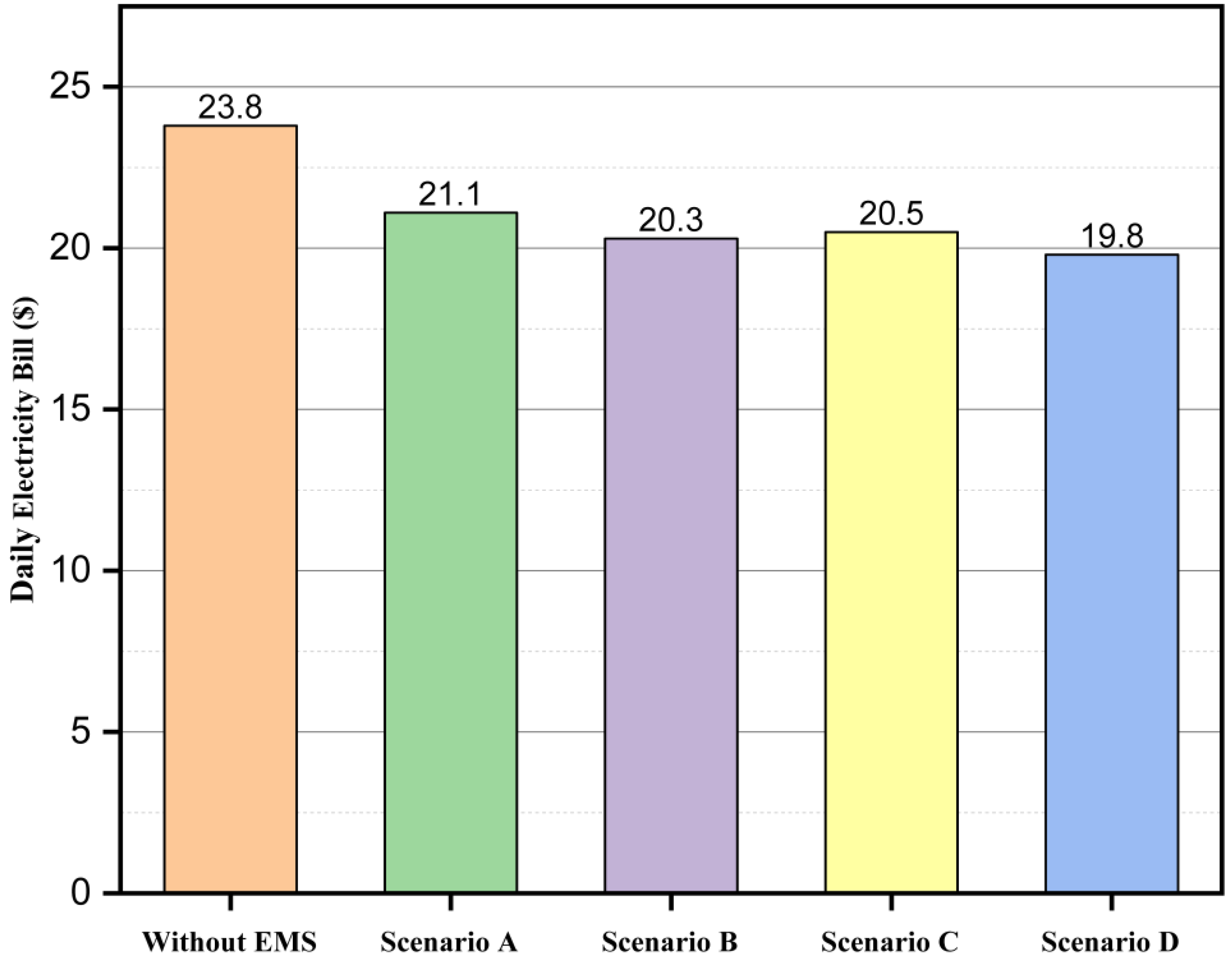
Transferring valley electricity through V2H proved to be more effective in reducing household electricity costs compared to transferring valley electricity through HESS alone.
Transferring valley electricity by HESS flattens the load curve better than transferring valley electricity through V2H.
Combining the transfer of valley electricity through V2H and HESS led to improved load curve flattening and reduced household electricity costs compared to either V2H or HESS alone.
The results highlighted the advantages of incorporating V2H and HESS systems into smart home. Thus, the research contributes to the creation of effective and sustainable smart home energy management systems by offering valuable insights on how to optimize energy usage, cut expenses, and achieve load curve smoothing.

Author Contributions

Conceptualization, M.A.A.A. and W.M.; methodology, M.A.A.A. and W.M.; software, M.A.A.A. and B.S.; validation, M.A.A.A., W.M. and B.S.; writing—original draft preparation, M.A.A.A.; writing—review and editing, G.A.A., A.A., O.A.A.M., H.A. and B.S.; supervision, W.M.; funding acquisition, A.A. and H.A. All authors have read and agreed to the published version of the manuscript.

Funding

This research was funded by the Researchers Supporting Project number (RSP2023R244), King Saud University, Riyadh, Saudi Arabia.

Conflicts of Interest

The authors declare no conflict of interest.

Abbreviations/Nomenclature

DODDepth of discharge
DERDistributed energy resources
ESSEnergy storage system
HESSHousehold energy storage system
EVsElectric vehicles
HEMSHome energy management system
SOCState of charge
TOUTime-of-use
V2HVehicle-to-home
V2GVehicle-to-grid
V2NVehicle-to-neighbor
Parameters
B R HESS rated discharge power (kW)
C B HESS one-time installation cost ($/kWh)
C D B Daily capital cost for HESS installation ($/day)
C E V EV battery replacement cost ($/kWh)
C D E V Daily EV battery degradation cost ($/day)
C D T Total daily energy consumption cost ($/day)
C D T , S A Total daily energy consumption cost in scenario A ($/day)
C D T , S B Total daily energy consumption cost in scenario B ($/day)
C D T , S C Total daily energy consumption cost in scenario C ($/day)
C D T , S D Total daily energy consumption cost in scenario D ($/day)
C f Number of possible full cycles during a battery lifetime
D Vehicle travel distance (km)
E R E V Required energy for the EV travel distance in the typical day (kWh)
E V R Rated charge power of EV (kW)
N Lifespan (years)
N d a y s Total number of days in the year
P a v g Daily average energy consumption by EV and household appliances (kW)
P B L t Power from the HESS to load (kW)
P E V L t Power from the vehicle to load (kW)
P G B t Power from the grid to HESS (kW)
P G E V t Power from the grid to vehicle (kW)
P L t Energy consumption of the household appliances at time interval t (kW)
P L n t New household power load curve (kW)
Q r a t e d B Rated capacity of the HESS (kWh)
Q r a t e d E V Rated capacity of the EV battery (kWh)
r Interest rate
S O C max B HESS maximum SOC (%)
S O C min B HESS minimum SOC (%)
S O C B t HESS SOC at a time interval t (%)
S O C B t 1 Previous HESS SOC (%)
S O C max E V EV maximum SOC (%)
S O C min E V EV minimum SOC (%)
S O C R E V Required SOC for the EV trip distance (%)
S O C E V t EV battery state of charge at time t (%)
S O C E V t 1 EV battery state of charge at the previous interval (%)
S O C E V t 0 Initial SOC of the EV battery
t a Arrival time
t d Departure time
W D Total energy consumption of household appliances throughout the day (kWh)
η c B HESS charge efficiency
η d B HESS discharge efficiency
η c E V EV battery charge efficiency
η d E V EV battery discharge efficiency
η V Vehicle efficiency (kWh/km)
λ t 
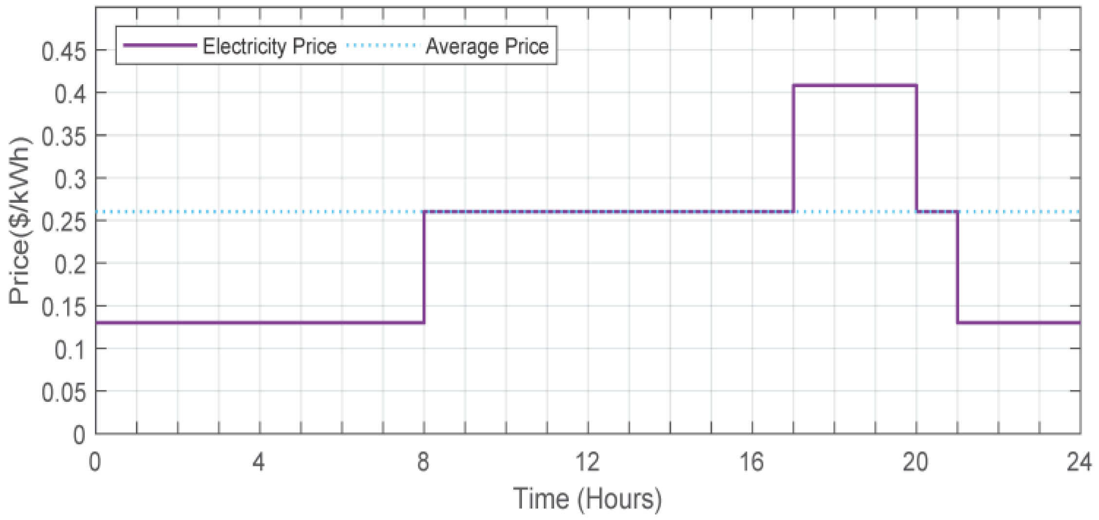
Price of electricity during different periods ($/kWh)
λ a v g Average electricity price ($/kWh)
λ m i d t Electricity price during mid-peak period ($/kWh)
λ o f f t Price of electricity during off-peak period ($/kWh)
λ o n t Electricity price during on-peak period ($/kWh)

References

  1. Shakeri, M.; Shayestegan, M.; Abunima, H.; Reza, S.M.S.; Akhtaruzzaman, M.; Alamoud, A.R.M.; Sopian, K.; Amin, N. An Intelligent System Architecture in Home Energy Management Systems (HEMS) for Efficient Demand Response in Smart Grid. Energy Build. 2017, 138, 154–164. [Google Scholar] [CrossRef]
  2. Zhou, B.; Li, W.; Chan, K.W.; Cao, Y.; Kuang, Y.; Liu, X.; Wang, X. Smart Home Energy Management Systems: Concept, Configurations, and Scheduling Strategies. Renew. Sustain. Energy Rev. 2016, 61, 30–40. [Google Scholar] [CrossRef]
  3. Zhao, G.Y.; Liu, Z.Y.; He, Y.; Cao, H.J.; Guo, Y.B. Energy Consumption in Machining: Classification, Prediction, and Reduction Strategy. Energy 2017, 133, 142–157. [Google Scholar] [CrossRef]
  4. Bagdadee, A.H.; Li, Z.; Abdalla, M.A.A. Constant &Reliable Power Supply by the Smart Grid Technology in Modern Power System. In IOP Conference Series: Materials Science and Engineering, Proceedings of the First International Conference on Materials Science and Manufacturing Technology, Coimbatore, India, 12–13 April 2019; IOP Publishing: Bristol, UK, 2019; Volume 561, p. 012088. [Google Scholar]
  5. Martinopoulos, G. Are Rooftop Photovoltaic Systems a Sustainable Solution for Europe? A Life Cycle Impact Assessment and Cost Analysis. Appl. Energy 2020, 257, 114035. [Google Scholar] [CrossRef]
  6. Nejat, P.; Jomehzadeh, F.; Taheri, M.M.; Gohari, M.; Majid, M.Z.A. A Global Review of Energy Consumption, CO2 Emissions and Policy in the Residential Sector (with an Overview of the Top Ten CO2 Emitting Countries). Renew. Sustain. Energy Rev. 2015, 43, 843–862. [Google Scholar] [CrossRef]
  7. Meng, K.; Dong, Z.Y.; Xu, Z.; Zheng, Y.; Hill, D.J. Coordinated Dispatch of Virtual Energy Storage Systems in Smart Distribution Networks for Loading Management. IEEE Trans. Syst. Man Cybern. Syst. 2017, 49, 776–786. [Google Scholar] [CrossRef]
  8. Wang, M.; Abdalla, M.A.A. Optimal Energy Scheduling Based on Jaya Algorithm for Integration of Vehicle-to-Home and Energy Storage System with Photovoltaic Generation in Smart Home. Sensors 2022, 22, 1306. [Google Scholar] [CrossRef]
  9. Berrada, A.; Loudiyi, K.; Zorkani, I. Profitability, Risk, and Financial Modeling of Energy Storage in Residential and Large Scale Applications. Energy 2017, 119, 94–109. [Google Scholar] [CrossRef]
  10. Wu, W.; Lin, B. Application Value of Energy Storage in Power Grid: A Special Case of China Electricity Market. Energy 2018, 165, 1191–1199. [Google Scholar] [CrossRef]
  11. Nguyen, H.K.; Bin, S.J.; Han, Z. Distributed Demand Side Management with Energy Storage in Smart Grid. IEEE Trans. Parallel Distrib. Syst. 2014, 26, 3346–3357. [Google Scholar] [CrossRef]
  12. Kittner, N.; Lill, F.; Kammen, D.M. Energy Storage Deployment and Innovation for the Clean Energy Transition. Nat. Energy 2017, 2, 17125. [Google Scholar] [CrossRef]
  13. Dharmakeerthi, C.H.; Mithulananthan, N.; Saha, T.K. Impact of Electric Vehicle Fast Charging on Power System Voltage Stability. Int. J. Electr. Power Energy Syst. 2014, 57, 241–249. [Google Scholar] [CrossRef]
  14. Wu, X.; Hu, X.; Yin, X.; Moura, S.J. Stochastic Optimal Energy Management of Smart Home with PEV Energy Storage. IEEE Trans. Smart Grid 2016, 9, 2065–2075. [Google Scholar] [CrossRef]
  15. Abdalla, M.A.A.; Min, W.; Haroun, A.H.G.; Elhindi, M. Optimal Energy Scheduling Strategy for Smart Charging of Electric Vehicles from Grid-Connected Photovoltaic System. In Proceedings of the 2021 7th International Conference on Electrical, Electronics and Information Engineering (ICEEIE), Malang, Indonesia, 2 October 2021; IEEE: New York, NY, USA, 2021; pp. 37–42. [Google Scholar]
  16. Leadbetter, J.; Swan, L. Battery Storage System for Residential Electricity Peak Demand Shaving. Energy Build. 2012, 55, 685–692. [Google Scholar] [CrossRef]
  17. Zurfi, A.; Albayati, G.; Zhang, J. Economic Feasibility of Residential Behind-the-Meter Battery Energy Storage under Energy Time-of-Use and Demand Charge Rates. In Proceedings of the 2017 IEEE 6th international conference on renewable energy research and applications (ICRERA), San Diego, CA, USA, 5–8 November 2017; IEEE: New York, NY, USA, 2017; pp. 842–849. [Google Scholar]
  18. Arcos-Vargas, A.; Lugo, D.; Núñez, F. Residential Peak Electricity Management. A Storage and Control Systems Application Taking Advantages of Smart Meters. Int. J. Electr. Power Energy Syst. 2018, 102, 110–121. [Google Scholar] [CrossRef]
  19. Gazafroudi, A.S.; Soares, J.; Ghazvini, M.A.F.; Pinto, T.; Vale, Z.; Corchado, J.M. Stochastic Interval-Based Optimal Offering Model for Residential Energy Management Systems by Household Owners. Int. J. Electr. Power Energy Syst. 2019, 105, 201–219. [Google Scholar] [CrossRef]
  20. Setlhaolo, D.; Xia, X. Optimal Scheduling of Household Appliances with a Battery Storage System and Coordination. Energy Build. 2015, 94, 61–70. [Google Scholar] [CrossRef]
  21. Longe, O.M.; Ouahada, K.; Rimer, S.; Harutyunyan, A.N.; Ferreira, H.C. Distributed Demand Side Management with Battery Storage for Smart Home Energy Scheduling. Sustainability 2017, 9, 120. [Google Scholar] [CrossRef]
  22. Sharifi, A.H.; Maghouli, P. Energy Management of Smart Homes Equipped with Energy Storage Systems Considering the PAR Index Based on Real-Time Pricing. Sustain. Cities Soc. 2019, 45, 579–587. [Google Scholar] [CrossRef]
  23. Yoon, S.-G.; Choi, Y.-J.; Park, J.-K.; Bahk, S. Stackelberg-Game-Based Demand Response for at-Home Electric Vehicle Charging. IEEE Trans. Veh. Technol. 2015, 65, 4172–4184. [Google Scholar] [CrossRef]
  24. Ahmed, M.S.; Mohamed, A.; Homod, R.Z.; Shareef, H. A Home Energy Management Algorithm in Demand Response Events for Household Peak Load Reduction. PrzeglAd Elektrotechniczny 2017, 93, 2017. [Google Scholar] [CrossRef]
  25. Zhang, W.; Zhang, D.; Mu, B.; Wang, L.Y.; Bao, Y.; Jiang, J.; Morais, H. Decentralized Electric Vehicle Charging Strategies for Reduced Load Variation and Guaranteed Charge Completion in Regional Distribution Grids. Energies 2017, 10, 147. [Google Scholar] [CrossRef]
  26. Khemakhem, S.; Rekik, M.; Krichen, L. A Flexible Control Strategy of Plug-in Electric Vehicles Operating in Seven Modes for Smoothing Load Power Curves in Smart Grid. Energy 2017, 118, 197–208. [Google Scholar] [CrossRef]
  27. Khemakhem, S.; Rekik, M.; Krichen, L. Double Layer Home Energy Supervision Strategies Based on Demand Response and Plug-in Electric Vehicle Control for Flattening Power Load Curves in a Smart Grid. Energy 2019, 167, 312–324. [Google Scholar] [CrossRef]
  28. Pal, S.; Kumar, R. Electric Vehicle Scheduling Strategy in Residential Demand Response Programs with Neighbor Connection. IEEE Trans. Ind. Inform. 2017, 14, 980–988. [Google Scholar] [CrossRef]
  29. Datta, U.; Saiprasad, N.; Kalam, A.; Shi, J.; Zayegh, A. A Price-regulated Electric Vehicle Charge-discharge Strategy for G2V, V2H, and V2G. Int. J. Energy Res. 2019, 43, 1032–1042. [Google Scholar] [CrossRef]
  30. Pearre, N.S.; Ribberink, H. Review of Research on V2X Technologies, Strategies, and Operations. Renew. Sustain. Energy Rev. 2019, 105, 61–70. [Google Scholar] [CrossRef]
  31. Melhem, F.Y.; Grunder, O.; Hammoudan, Z.; Moubayed, N. Optimization and Energy Management in Smart Home Considering Photovoltaic, Wind, and Battery Storage System with Integration of Electric Vehicles. Can. J. Electr. Comput. Eng. 2017, 40, 128–138. [Google Scholar] [CrossRef]
  32. Aznavi, S.; Fajri, P.; Asrari, A.; Harirchi, F. Realistic and Intelligent Management of Connected Storage Devices in Future Smart Homes Considering Energy Price Tag. IEEE Trans. Ind. Appl. 2020, 56, 1679–1689. [Google Scholar] [CrossRef]
  33. Huang, P.; Lovati, M.; Zhang, X.; Bales, C. A Coordinated Control to Improve Performance for a Building Cluster with Energy Storage, Electric Vehicles, and Energy Sharing Considered. Appl. Energy 2020, 268, 114983. [Google Scholar] [CrossRef]
  34. Farsangi, A.S.; Hadayeghparast, S.; Mehdinejad, M.; Shayanfar, H. A Novel Stochastic Energy Management of a Microgrid with Various Types of Distributed Energy Resources in Presence of Demand Response Programs. Energy 2018, 160, 257–274. [Google Scholar] [CrossRef]
  35. Abdalla, M.A.A.; Min, W.; Mohammed, O.A.A. Two-Stage Energy Management Strategy of EV and PV Integrated Smart Home to Minimize Electricity Cost and Flatten Power Load Profile. Energies 2020, 13, 6387. [Google Scholar] [CrossRef]
  36. Hot Purple Energy Southern California Edison Strikes Again with New Time-of-Use Rate Structure. Available online: https://hotpurpleenergy.com/sce-new-rate-structure/ (accessed on 1 February 2023).
  37. U.S. Energy Information Administration Hourly Electricity Consumption Varies throughout the Day and across Seasons. Available online: https://www.eia.gov/todayinenergy/detail.php?id= (accessed on 1 February 2023).
  38. Young, K.; Wang, C.; Wang, L.Y.; Strunz, K. Electric Vehicle Battery Technologies. In Electric Vehicle Integration into Modern Power Networks (Power Electronics and Power Systems); Springer: New York, NY, USA, 2013; pp. 15–56. [Google Scholar]
  39. McGuckin, N.A.; Fucci, A. Summary of Travel Trends: 2017 National Household Travel Survey; US Department of Transportation, Federal Highway Administration: Washington, DC, USA, 2018.
Figure 1. Smart home schematic diagram.
Sustainability 15 15046 g001
Figure 2. The energy scheduling strategy flowchart for EV charging without V2H and HESS.
Sustainability 15 15046 g002
Figure 3. The energy scheduling strategy flowchart for EV charging with V2H without HESS.
Sustainability 15 15046 g003
Figure 4. The energy scheduling strategy flowchart for EV charging with HESS without V2H.
Sustainability 15 15046 g004
Figure 5. The energy scheduling strategy flowchart for EV charging with V2H and HESS.
Sustainability 15 15046 g005
Figure 6. Residential electricity prices curve.
Sustainability 15 15046 g006
Figure 7. Daily electricity consumption.
Sustainability 15 15046 g007
Figure 8. The transitions between different modes during the day in (a) scenario A, (b) scenario B, (c) scenario C, and (d) scenario D.
Sustainability 15 15046 g008
Figure 9. EV SOC in (a) scenario A, (b) scenario B, (c) scenario C, and (d) scenario D.
Sustainability 15 15046 g009
Figure 10. HESS SOC in (a) scenario C and (b) scenario D.
Sustainability 15 15046 g010
Figure 11. EV battery current curves in (a) scenario A, (b) scenario B, (c) scenario C, and (d) scenario D.
Sustainability 15 15046 g011
Figure 12. HESS current curves in (a) scenario C and (b) scenario D.
Sustainability 15 15046 g012
Figure 13. EV power curve in (a) scenario A, (b) scenario B, (c) scenario C, and (d) scenario D.
Sustainability 15 15046 g013
Figure 14. HESS power curve in (a) scenario C and (b) scenario D.
Sustainability 15 15046 g014
Figure 15. Power load profile comparison.
Sustainability 15 15046 g015
Figure 16. Daily electricity bill comparison.
Sustainability 15 15046 g016
Table 1. This table represent scenario in terms of the objectives and constraints.
ScenarioObjectivesConstraints
Scenario 1
  • Control Charging of EV to reduce the load variation and electricity bill.
  • The EV battery charge when the price and consumption of the electricity are low.
  • EV SOC should not exceed upper limits.
Scenario 2
  • Control Charging/discharging of EV with aim of reduce the load variation and electricity bill.
  • The EV battery charge if the price and consumption of the electricity are low.
  • EV battery discharge during the peak load period only.
  • EV battery SOC at departure time should be equal or higher than the required SOC for the EV trip distance.
  • EV SOC should not exceed upper and lower limits.
Scenario 3
  • Control of EV charging.
  • Control of HESS Charge/discharge.
  • Reduce the load variation and electricity bill.
  • The EV battery and HESS are charge if the price and consumption of the electricity are low.
  • The HESS discharge during the peak load period only.
  • Giving priority to charging EV before HESS.
  • The SOC of the EV battery and the HESS should not exceed the SOC upper and lower limits to prevent over-charge/discharge.
Scenario 4
  • Control of EV Charge/discharge.
  • Control of HESS Charge/discharge.
  • Reduce the load variation and electricity bill.
  • The EV battery and HESS are charge if the price and consumption of the electricity are low.
  • The HESS and EV battery should discharge during the peak load period only.
  • Giving priority to charging EV before HESS.
  • Giving priority to discharge HESS before EV.
  • The SOC of the EV battery and the HESS should not exceed the SOC upper and lower limits to prevent over-charge/discharge.
  • EV battery SOC at departure time should be equal or higher than the required SOC for the EV trip distance.
Table 2. Residential electricity prices.
PeriodsElectricity Price ($/kWh)
On-peak0.40824
Mid-peak0.26018
Off-peak0.12995
Table 3. EV and HESS parameters.
DescriptionEVHESS
Battery capacity19 kWh8.64 kWh
S O C max 90%90%
S O C min 20%20%
Initial SOC50%50%
Depth of discharge DOD80%80%
Charging efficiency η c 0.950.90
Discharging efficiency η d 0.950.90
Max power1.6 kW1.2 kW
Min power−1.5 kW−1.0 kW
Vehicle depart time08:00-
Vehicle arrive time17:00-
Vehicle efficiency η V 14 kWh/100 km-
Table 4. Economic parameters associated with the HESS and EV battery.
ComponentParametersValueUnit
HESSInvestment cost150$/kWh
HESS system lifetime N10years
EV batteryReplacement cost200$/kWh
Cycle life2000Cycles
OtherInterest rate (r)6%
Table 5. Comparison of the proposed strategy with the existing literature.
Ref.ObjectivesStorage Technologies
Minimize Peak LoadSmoothing Load CurveReduce CostHESSEV
[16]---
[17]---
[20]--
[23]---
[26]--
[28]--
[31]--
This study
Disclaimer/Publisher’s Note: The statements, opinions and data contained in all publications are solely those of the individual author(s) and contributor(s) and not of MDPI and/or the editor(s). MDPI and/or the editor(s) disclaim responsibility for any injury to people or property resulting from any ideas, methods, instructions or products referred to in the content.

