Article

Assessing Shock Propagation and Cascading Uncertainties Using the Input–Output Framework: Analysis of an Oil Refinery Accident in Singapore

by
Pradeep V. Mandapaka
1,* and
Edmond Y. M. Lo
1,2,*
1
Institute of Catastrophe Risk Management, Nanyang Technological University, 50 Nanyang Avenue, Singapore 639798, Singapore
2
School of Civil and Environmental Engineering, Nanyang Technological University, 50 Nanyang Avenue, Singapore 639798, Singapore
*
Authors to whom correspondence should be addressed.
Sustainability 2023, 15(2), 1739; https://doi.org/10.3390/su15021739
Submission received: 12 December 2022 / Revised: 13 January 2023 / Accepted: 13 January 2023 / Published: 16 January 2023

Abstract

:
The impacts of shock events frequently cascade beyond the primarily affected sector(s), through the interdependent economic system, and result in higher-order indirect losses in other sectors. This study employed the inoperability input–output model (IIM) and the dynamic IIM (DIIM) to model recovery of sectors after a shock event and quantify associated total losses. Considering data limitations and uncertainties regarding sectoral recovery time, a key variable in DIIM, a probabilistic approach is used for modelling uncertainty in recovery times. The event analyzed is the 2011 oil refinery fire accident in Pulau Bukom (PB) island, Singapore, which caused the refinery to shut down for 11 days and be partially operational for several days thereafter. The impacts are assessed using the regrouped 15-sector Singapore IO data of year 2010, with manufacturing sector as the directly affected sector. The initial economic impact of the PB refinery fire is assessed in the top-down framework using the refinery’s contribution to the manufacturing sector and nation’s GDP. The higher-order losses are quantified considering different recovery paths for the directly affected sector and accounting for its inventory. Simulation experiments using synthetic IO tables are also carried out to understand relationship between recovery characteristics of directly and indirectly affected sectors. The results from IIM analysis show that the indirect losses are about 35–38% of direct losses. The DIIM analysis reveal that the utilities sectors (e.g., electricity, water supply and treatment) suffer the largest inoperability among indirectly affected sectors for a given direct damage to the manufacturing sector. The results also illustrate the dependence of overall losses on the recovery path of the directly affected sector, and associated uncertainties in sectoral recovery times.

1. Introduction

The impacts of disasters are not just limited to stock damages and direct flow losses, but also include indirect losses because of interdependent physical and economic systems [1,2,3,4]. Due to increasingly interdependent infrastructure and social, and economic systems, a shock-event-induced disruption in one system can rapidly cascade to other systems and increase total losses [5,6,7,8,9]. The indirect loss component can vary considerably depending on the dynamics of the recovery process, which further depend on the pace of restoration and reconstruction efforts and the strength of interdependencies among different systems. For example, at the aggregated scale of economic sectors, the recovery dynamics depend on factors such as linkages with the primarily affected sector(s) and associated supply–demand imbalances, access to labor supply and critical infrastructure services, and availability of substitutes [10,11]. Because of the multitude of interacting and often uncertain factors, there is a significant uncertainty in modelling the overall recovery process, which propagates into estimates of indirect losses. For Hurricane Sandy, Kunz, et al. [7] estimated that a direct loss of 9.4 billion in the manufacturing sector led to an indirect loss in the range of $1.4–5.6 billion depending on recovery scenario. For two simulated flood scenarios in Northern Italy, Koks, et al. [12] showed that economic loss estimates depend strongly on the recovery path, especially in the affected region. The indirect loss due to the 2008 Sichuan earthquake was estimated to be about the same as the direct loss for Sichuan province but was more than twice that at the national level [13].
The above highlights the importance of modelling the propagation of shock-induced production and service disruptions and associated recovery uncertainties when characterizing the resilience of a system to shock events. A thorough understanding of the interdependencies and their effect on shock propagation under different recovery scenarios will benefit risk management practices as well as supporting decision makers by providing an integrated, system-wide view of disaster impacts. The current paper recognizes this and analyses the impact of recovery dynamics and uncertainties on overall loss estimates using a real case of an oil refinery fire accident in Singapore. The fire accident on Singapore’s Pulau Bukom (PB) island caused the refinery to shut down for 11 days and be partially operational for several days following the fire, [14]. This study accounts for sectoral interdependencies as well as multiple recovery paths and investigates the role of preparedness measures (e.g., inventory) while quantifying the range of overall losses from the refinery accident to the individual sectors and to the economy.
The input–output (IO) and computable general equilibrium (CGE) models are the two widely used approaches to assess indirect economic losses due to a disaster [12,15,16,17]. The IO database provides a detailed empirical representation of the flow of goods and services among interdependent industrial sectors and end users [18,19]. The IO models are thus well-suited to understand sectoral interdependencies and offer simple yet elegant means to examine how a disruption in one sector propagates among sectors and into the economy. However, IO models have well-known limitations such as rigid structure, linearity of interdependencies, and lack of substitution among inputs [20,21]. Despite these caveats, IO models have been used extensively in disaster analyses, where they are extended and integrated with engineering, econometric, and network-based models [17,22]. CGE models, on the other hand, are more flexible than IO models, as they can accommodate nonlinear production and consumption functions, input and import substitution possibilities, resource constraints, and consumer behavior in response to, e.g., changes in prices [23,24,25]. However, the CGE models are complex and data intensive, with required data difficult to obtain for many disaster scenarios [20,25,26].
In this study, we use the inoperability IO model (IIM) and its temporal extension, the dynamic inoperability IO model (DIIM) [27,28], which are widely used for disaster impact analysis, including the impacts of pandemics [29,30], floods [31,32], landslides [33], and power outages [34,35]. Section 2 describes the models and uncertainties used in this study. The IO data and the overall cost and use structure of production in Singapore are described in Section 3. The PB refinery fire and its initial impact are described in Section 4, while its higher-order impacts on the economy obtained via static and dynamic IO models are discussed in Section 5, including effects of recovery shape. This is followed by concluding remarks in Section 6.

2. Methodology

A short description of the classical Leontief IO model [18,19] is provided first as it forms the basis for the models used in this study.

2.1. Leontief IO Model

The main components of the Leontief IO framework are the intersectoral transactions (e.g., purchases, sales by sectors during production), the primary inputs (e.g., labor, capital), and the final demand of the end users. At equilibrium, the Leontief IO model is written as x = A · x + f [19], where x is a vector storing annual economic output of each sector, A is the technical coefficients matrix, and f is a vector containing the final consumption requirements of the end users. Each element a i j in A quantifies the amount of input required from sector i to sector j to produce a dollar output of sector j. The above equation can be rearranged as x = I A 1 f , where I A 1 is called the total requirements matrix or the Leontief inverse. If the initial effect of a shock event is quantified in terms of a change in the final demand Δ f , then the overall economic impact Δ x induced by Δ f is computed using:
Δ x = I A 1 Δ f

2.2. Inoperability IO Model (IIM)

Building upon the Leontief IO model, Haimes and Jiang [36] proposed the IIM for interconnected infrastructure systems, which was refined by Santos and Haimes [37] by modelling interdependencies using readily available economic transactions data. Inoperability is defined as the inability of a sector to produce its planned output. If x i and x ˜ i are outputs of sector i under normal and disrupted scenarios, respectively, then inoperability q i is the ratio of unrealized to planned production, x i x ˜ i / x i , with 0 q i 1 . The demand-reduction IIM is written as q = A * · q + c * and rearranged as [37]:
q = I A * 1 c *
A * is the interdependency matrix obtained as A * = x ^ 1 A x ^ , and c * is the normalized demand perturbation vector obtained as c * = x ^ 1 Δ f , where x ^ is the diagonal matrix containing sectoral output x along the diagonal. Previous applications of IIM include studying the impacts of terrorism-related disruptions [37], hurricanes [38], and power blackouts [6]. The sector inoperabilities for a given demand perturbation can also be obtained by normalizing the output from the Leontief IO model (Equation (1)), as illustrated by Dietzenbacher and Miller [39]. The IIM version is used for the static analysis in this study as it sets the foundation for the temporal version described next.

2.3. Dynamic Inoperability IO Model (DIIM)

The IO and IIM models lack a temporal component, which limits their application to study the recovery process. The DIIM proposed by Lian and Haimes [28] is a widely used extension of IIM for studying the temporal evolution of inoperabilities. For a given initial inoperability q 0 and demand perturbation c * 0 , the DIIM constructs the inoperability trajectory in time t as [28]:
q t + 1 = q t + K A * q t + c * t q t
where K is the diagonal matrix of sector recovery coefficients k i i . Following Jonkeren and Giannopoulos [40], we use the term recovery coefficients to describe k i i instead of the commonly used resilience coefficients. Equation (3) can be written in scalar form as q i t + 1 = q i t + k i i j = 1 n a i j * q j t + c i * t q i t . As 0 q i 1     i , it is the term in parenthesis that determines whether a sector is in recovery mode (decreasing inoperability) or otherwise.

2.3.1. Recovery Coefficients and Uncertainty Modelling

The diagonal element k i i in K describes the ability of sector i to recover from a shock-induced supply–demand imbalance, and is obtained as [28]:
k i i = ln q i 0 / q i t T i 1 1 a i i *
where T i is the time taken by sector i to recover from an initial inoperability of q i 0 to a desired post-recovery inoperability q i T i and a i i * is the sector’s self-dependency element in A * . Thus, for a given A * , recovery time plays a crucial role in determining the inoperability trajectory of each sector. As historical data on T i for different shock events are scarce, studies typically rely on assumptions or expert opinions to estimate T i [28,31,34]. Recognizing the challenges associated with quantifying T i , we take the probabilistic approach and assume that a sector’s time to recover from a q i 0 of 100% to a post-recovery inoperability of 1% follows a PERT distribution, a version of Beta distribution [41]. As T i is typically based on expert opinions/estimates, which come in the form of a range (minimum, maximum) and the most likely value, a bounded distribution such as PERT distribution is chosen in this study. Unlike a triangular distribution, which requires the same three parameters (minimum, mode, maximum), a PERT distribution has lighter tails and gives greater weight to the most likely value. PERT distributions have been employed to model expert opinions in various areas including flood susceptibility analysis [42], land suitability for crops [43], and, related to the current study, recovery times of economic sectors [44].
A PERT distribution bounded between a and c , with a mode at b and a mean at a + 4 b + c / 6 , is related to the Beta distribution as P E R T a , b , c = a + c a B e t a α 1 , α 2 , where α 1 = 1 + 4 b a c a and α 2 = 1 + 4 c b c a . For each sector i, we assumed that its most likely (i.e., mode) recovery time T ´ i is a function of a i i * as follows.
T ´ i = 15 / a i i *
Using this mode value and setting the lower and upper bounds to 0.5 T ´ i and 1.5 T ´ i , 1000 values of T i from a PERT distribution are generated for each sector, resulting in 1000 T vectors.

2.3.2. DIIM Extensions

The DIIM was extended over the years to account for international trade [45], inventories [46], and uncertainties [44]. We employ the extension proposed by Barker and Santos [46], which accounts for a sector’s production inoperability ( p i t ) and available inventory ( s i t ) before determining the overall inoperability as described by the following three cases.
q i t + 1 = { q i t + k i i j = 1 n a i j * q j t + c i * t q i t 1 :   s i t + 1 p i t + 1 x i t + 1 max q i t + k i i j = 1 n a i j * q j t + c i * t q i t p i t + 1 s i t + 1 / x i t + 1 2 :   i f   0 < s i t + 1 < p i t + 1 x i t + 1 max q i t + k i i j = 1 n a i j * q j t + c i * t q i t p i t + 1 3 :   i f   s i t + 1 = 0
p i t is defined as the inoperability of a sector i at time t due only to the direct disruption to the production process, and is independent of other sectors. By definition, p i t = 0     t for sectors that are not directly affected by a shock event. Exponential functions are commonly used to model p i t [46], but case-specific inputs can be provided if data are available. At each time step, when s i fully covers p i (Case 1, Equation (6)), the overall inoperability of a sector is same as the one obtained from standard DIIM (Equation (3) in scalar form). If s i covers only a part of p i (Case 2), then the overall inoperability is the maximum of standard DIIM-based inoperability and the residual p i . If s i is not available (Case 3), the overall inoperability is the maximum of standard DIIM-based inoperability and p i . The initial inoperability required to run Equation (6) is set as follows:
q i 0 = 0 i f   s i 0 p i 0 x i 0 p i 0 s i 0 x i 0 i f   0 < s i 0 < p i 0 x i 0 p i 0 i f   s i 0 = 0  
Assuming that the baseline annual output vector x is evenly distributed to 365 days, the inoperability vector q t at time t can be converted into post-shock economic output x ˜ t as:
x ˜ t = 1 365 x x ^ · q t

3. Singapore IO Data and Structure of the Economy

The IO data on intersectoral economic transactions for Singapore is distributed by the Department of Statistics, Singapore for 105 sectors [47]. We obtained the 2010 IO data for this study as it is the closest year preceding the PB refinery accident. The raw data on intersectoral transactions, the final demand f , and primary inputs v are then grouped into 15 broad sectors. Table A1 of Appendix A lists the 15 sectors and their component subsectors. The technical coefficients matrix A is calculated from the intersectoral transactions data, which is then used along with f and v in this study.
The total production in Singapore in year 2010 is $844.5 billion SGD (Singapore dollar hereafter) to which the manufacturing (MANUF) sector has the largest contribution ($295.3 billion or 35%) followed by the wholesale and retail (WHRTL) and professional and business services (PRBSN) sectors (Figure 1a). The percentage input requirements or the production costs for each sector are shown in Figure 1b. For example, to produce $100 of output, the MANUF sector requires $27 worth of inputs from domestic industries and $50 of imports and pays $7 towards income. Construction (CONST) and water supply and waste management (WTWST) are among the sectors that have larger domestic input requirements, whereas the MANUF and ELECT sectors have larger import requirements per unit output. The services sectors (e.g., EDUHS, OTHSV) dominate the payments made towards income. Figure 1c shows the usage of each sector’s output as intermediate consumption during the production process and for final demand by household, government consumption expenditure (GCE), and gross capital formation (GCF). About 25% of MANUF’s output is used by all sectors (incl. MANUF) for production, and a large fraction of the sector’s output is exported. Expectedly, a major part of CONST’s output goes towards GCF. Although utilities sectors (WTWST, ELECT, and GAS) have smaller outputs compared to many other sectors, they form an integral part of the production process. For example, about 84% of ELECT’s output is consumed by all sectors during the production stage.

4. Description of the PB Refinery Fire

Singapore is one of the major oil refining centers in the world, and is often referred to as Asia’s oil refining and trade hub [48,49]. With a total crude oil refining capacity of 1.43 million barrels per day (bpd), Singapore contributed 4.7% to the total refining capacity of Asia Pacific and 1.5% globally in year 2010 ([50], p. 31). The refinery by ExxonMobil on Jurong Island is among the largest in the world with a capacity of 592,000 bpd, thus accounting for about 41% of Singapore’s total refining capacity [51]. The Royal Dutch Shell refinery on PB island was the first refinery in Singapore, and is capable of processing up to 500,000 bpd, contributing 35% to Singapore’s total refining capacity in 2010 [52].
The 2011 PB refinery fire started at the refinery’s largest pump house on the afternoon of 28 September 2011, and escalated into a major blaze in the next 24 h [14,53]. The scale and complexity of the fire prompted the Singapore Civil Defence Force (SCDF) to declare Operations Civil Emergency, Singapore’s national response plan for civil emergencies [14], and the refinery was shut down progressively as a safety precaution. The fire was extinguished late in the evening of 29 September 2011 after 32 h of coordinated efforts by SCDF, Shell’s fire-fighting team, and multiple government agencies. Although the affected site was handed back to the refinery on 2 October, the operations remained shut down for the next one week. The refinery resumed at 20% capacity on 10 October 2011 [54], and gradually returned to full production capacity by the end of December 2011 [53]. The exact course of the refinery’s recovery back to normalcy is difficult to ascertain due to a lack of specific operational data.
The models described in Section 2 quantify the total economic impact for a given initial impact to the affected sector. The initial impact of the PB fire to the refinery sector is estimated here using the top-down approach, based on the sector’s relative contribution to the gross domestic product (GDP) of Singapore. The refining and production work is part of the chemicals cluster (comprising petroleum, petrochemicals, and other specialty chemicals), which in turn is part of the MANUF sector. As the analysis in this study is conducted using the IO data of 15 broadly organized sectors, the initial impact is considered to be only to the MANUF sector. In the year 2010, the MANUF sector contributed 22% to Singapore’s GDP of $327 billion [47,55], and the chemicals cluster accounted for about 10.4% of the MANUF sector [56]. In addition, the PB refinery contributed 35% to the nation’s total refining capacity. Combining this information, the initial daily impact of the PB fire to the MANUF sector is calculated as 1 365 × 0.35 × 0.104 × 0.22 × $ 327 , 000 = $ 7.17 million.

5. Results and Discussion

5.1. Static IIM

In the static IIM described in Section 2.2, the initial impact to the affected sector is entered into the model as a reduction in final demand (Section 2.2). The normalized demand perturbation for the MANUF sector, c m a n u f * , in the vector c * is calculated as Δ f m a n u f / x m a n u f = 7.17 / 809 = 0.0089 , where $809 million is the total daily output of the sector (Section 3). All other elements in c * are set to zero, as the initial impact is only to the MANUF sector. The demand perturbation in MANUF leads to inoperability in MANUF, which cascades to other sectors because of interdependencies. The sectoral inoperabilities are obtained from demand-driven IIM (Equation (2)) and multiplied with the corresponding daily pre-shock economic outputs to obtain sectoral economic losses.
Table 1 lists sectoral impacts ranked according to inoperability and corresponding daily economic loss. Results reveal that the initial demand reduction of 0.89% in the MANUF sector renders the sector inoperable by 1.08% but also causes other sectors to be inoperable. The top three inoperable sectors besides the primarily affected MANUF sector are the ELECT, GAS, and WTWST sectors. The WHRTL, PRBSN, and ELECT sectors are the top three indirectly affected sectors in terms of economic loss.
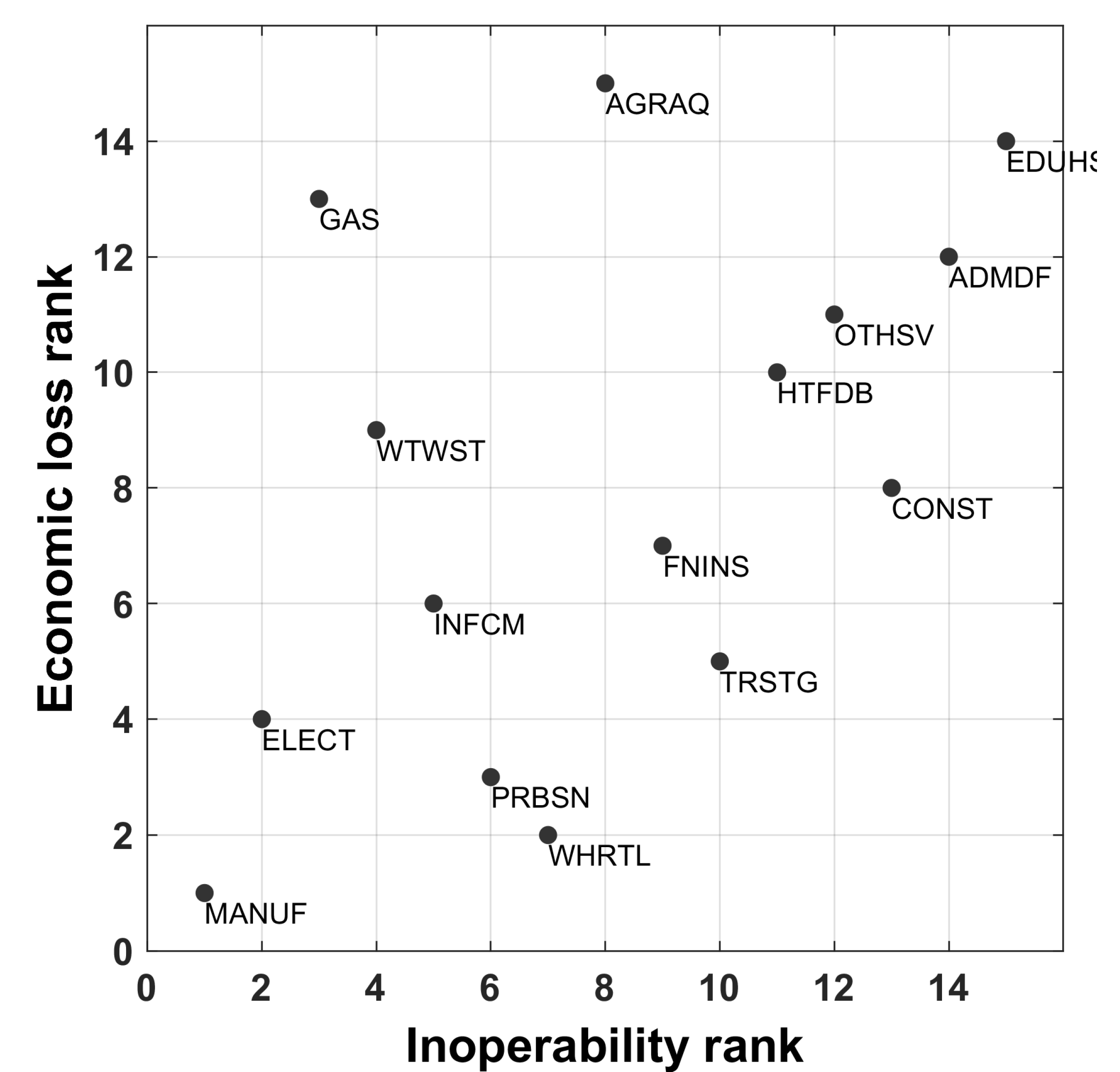
Figure 2 compares the sectors based on their inoperability and economic loss rankings. The directly affected MANUF sector ranks high on both metrics. Although utilities sectors such as GAS and WTWST rank high on the inoperability criterion, their economic loss ranking is low as their daily economic output is much smaller compared to other sectors (see Figure 1a). Similarly, WHRTL, PRBSN, and TRSTG rank higher on an economic loss basis as their economic output is larger. Overall, the total (initial + indirect) daily loss due to the PB fire incident assessed via static demand-driven IIM is $9.91 million, out of which the MANUF sector suffered $8.71 million or 87.9% of the total loss. The indirect losses were $9.91−$7.17 = $2.74 million or about 38% of the direct loss. For the same event, Lin, et al. [52] reported a total daily economic loss of $8.17 million. The smaller economic loss in Lin, et al. [52] compared to the current study is mainly due to the use of 2005 data for IO and GDP in their analysis.

5.2. Dynamic IIM

The temporal evolution of inoperabilities is assessed using the extended DIIM (Section 2.3.2), in which the initial impact on the directly affected sector is represented in terms of production inoperability and/or change in final demand. We assigned the PB fire-induced initial impact ($7.17 million) to the MANUF sector’s production inoperability as p m a n u f 0 = 7.17 / 809 = 0.89 % . The framework also requires the full trajectory of p m a n u f t , which we constructed using the information from Section 4 that the refinery was shut down on September 28 (Day 0) and resumed operations at 20% capacity on October 10. As data on refinery recovery from October 11 is not available, except that the plant was fully operational by December 2011, we assumed two exponential scenarios, a rapidly decaying (concave up) and a slowly decaying (concave down) p m a n u f t from Day 13. Similar trajectories, along with the simple linear path, have been employed to model sectoral recovery [12,40,46].

5.2.1. Rapid Initial Recovery of the MANUF Sector’s Production Inoperability

The complete trajectory of p m a n u f t , constructed using observed information until Day 12 followed by a concave-up recovery scenario from Day 13 is shown in Equation (9).
p m a n u f t = p m a n u f 0 i f   0 t 11     S e p   28 O c t   9   0.8 × p m a n u f 0 i f   t = 12   O c t   10 e k ˜ m a n u f t 12 p m a n u f 12 i f   t 13   f r o m   O c t   11
The rapid drop of p m a n u f t from Day 13 is modelled following Barker and Santos [46], where k ˜ m a n u f is the rate of repair, defined similarly to the recovery coefficient (Equation (4)) but without dependence on a i i * , i.e., k ˜ m a n u f = 1 / T m a n u f ln p i 0 / p i t . As the direct impact of the PB accident is assumed to be limited to the MANUF sector (Section 4), p i t = 0     t and i   MANUF. The assumption of zero production inoperabilities for non-MANUF sectors also implies that no other shock event has occurred and affected these sectors during the study timeframe. Further, the inventory available in each sector is assumed to be zero. Therefore, following Case 3 of Equation (6), the larger value among the standard DIIM-based inoperability and p m a n u f is taken as MANUF’s overall inoperability at each time step. While the former is computed considering interdependencies with all sectors, the latter is intrinsic to MANUF. The model is applied for the most likely recovery time vector T ´ (Equation (5)) and for 1000 T vectors generated from a PERT distribution (Section 2.3.1).
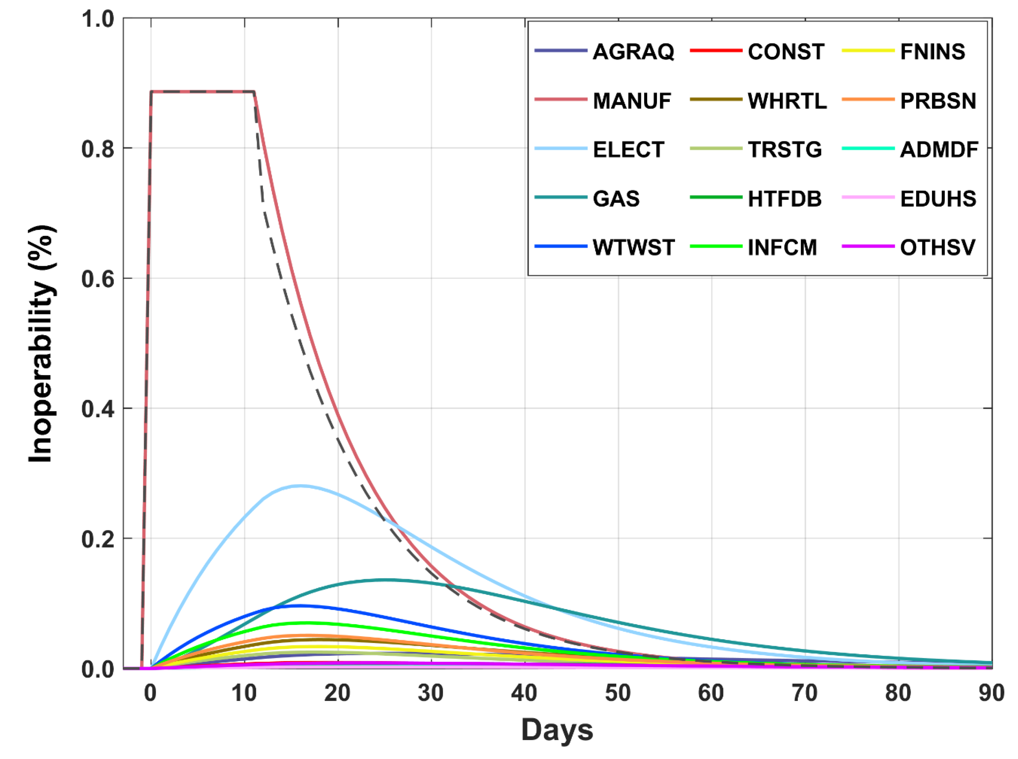
Figure 3 shows overall inoperability trajectories of each sector for the recovery scenario T ´ . For the MANUF sector, p m a n u f t (dashed line, Figure 3) is larger than the inoperability computed from standard DIIM until t = 11, and consequently chosen as the overall inoperability of the sector. For t > 11, the standard DIIM-based inoperability is larger than p m a n u f t , and thus determines the overall inoperability of the sector. Further, the MANUF sector recovers following an exponential trajectory from t > 12 as the general solution to the standard DIIM is an exponentially decaying function, [57]. For the indirectly affected sectors, as p i t = 0     t (i   MANUF), Case 3 of Equation (6) simplifies to standard DIIM. For example, the ELECT sector suffers only from interdependency-induced inoperability, which is captured by the standard DIIM. This inoperability increases during the initial time steps as j = 1 n a e l e c t , j * q j t > q e l e c t t (see Equation (6)) and reaches peak at t = 17 before starting on the recovery path from t = 18 (Figure 3). Among the indirectly affected sectors, the ELECT sector has the largest peak inoperability ( q p ) followed by the GAS and WTWST sectors.
To better understand the inoperability trajectories of indirectly affected sectors, we conducted simulations using synthetic two-sector and five-sector IO tables, the details of which are presented in Appendix B. Simulation results revealed that q p of an indirectly affected sector is larger when the sector’s recovery coefficient is larger combined with a smaller recovery coefficient for the directly affected sector (Figure A1 and Figure A2, Appendix B). Further, when all sectors have the same recovery coefficients, the q p of indirectly affected sectors are determined by the elements of the jth column of the matrix G = I A * 1 , where j is the directly affected sector (Figure A3, Appendix B). Specifically, the larger the G i , j , the higher the q p rank of an indirectly affected sector i (i     j).
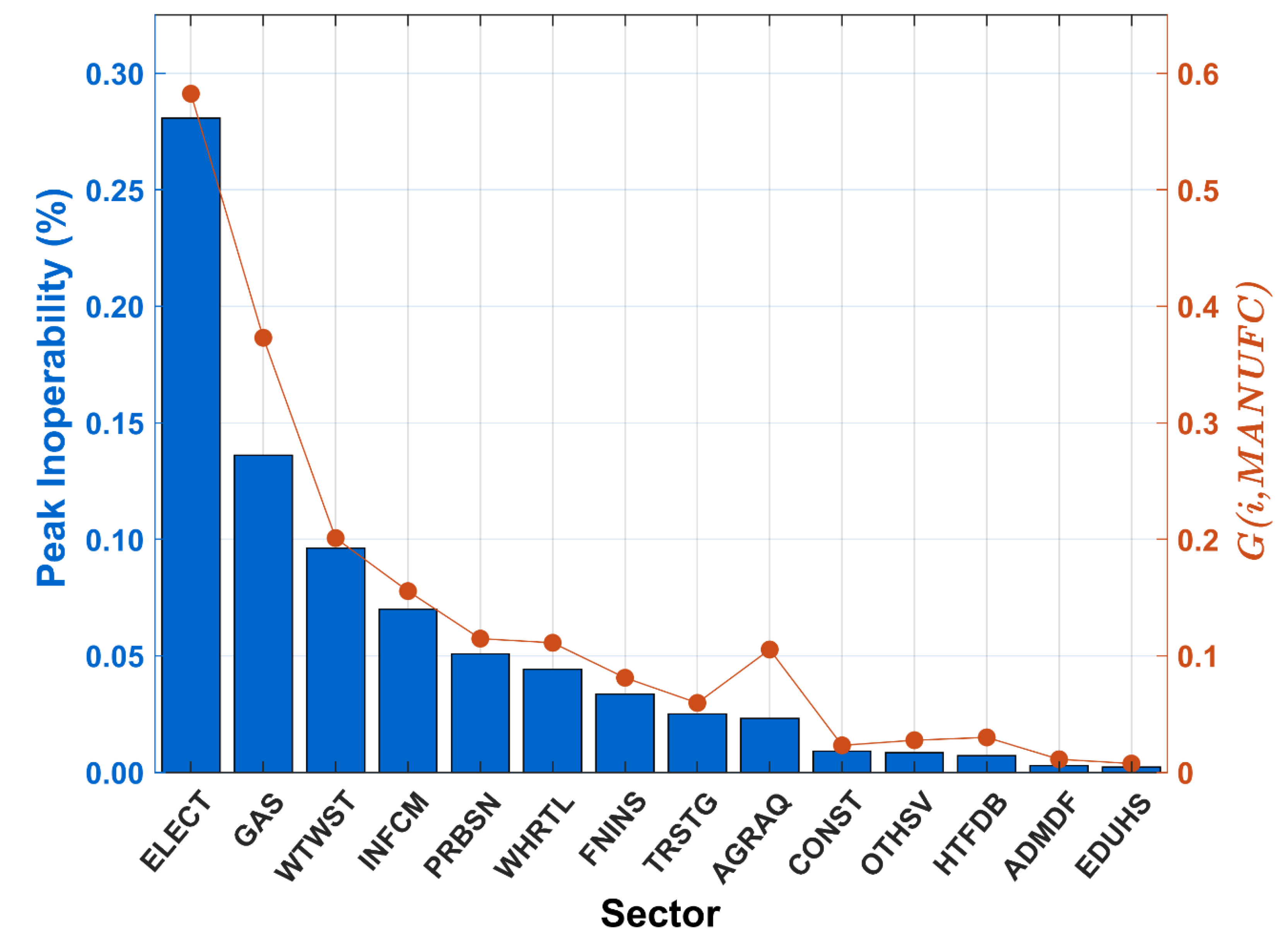
For Singapore’s economic sector, the recovery coefficients (from Equation (4)) do not show much variability. For example, the coefficients computed for the recovery time scenario T ´ have a coefficient of variation of 0.4. Thus, based on our findings from Figure A3, it is expected that the q p rank of an indirectly affected sector i is mainly determined by G i , j , where j is the directly affected sector. The q p of each indirectly affected sector i from Figure 3 is plotted in Figure 4 along with G i , M A N U F . In general, a sector with a larger value of G i , M A N U F has a larger q p , except for the AGRAQ sector, which is because of the sector’s much smaller recovery coefficient (0.023) compared to the average value of 0.079.
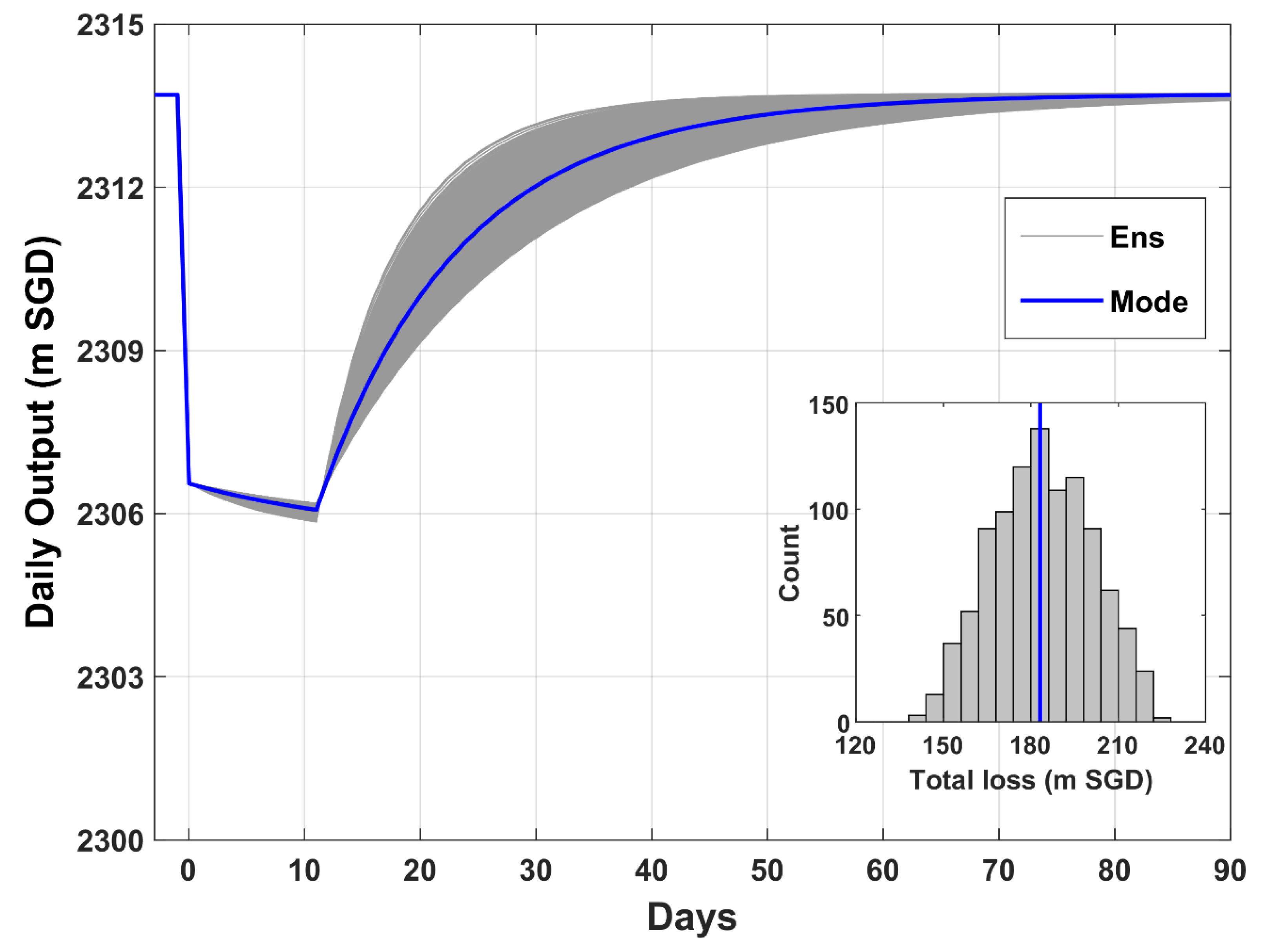
The sectoral inoperabilities q t are converted to corresponding economic outputs x ˜ t using Equation (8). Figure 5 shows the variation in total daily economic output, i.e., i = 1 15 x ˜ i t , for the recovery time vector T ´ and for 1000 PERT-distributed T vectors. At Day 0, there is a drop in total output because of the initial inoperability suffered by the MANUF sector. Although the MANUF sector’s inoperability stays flat until Day 12 (see Figure 3), the total daily output in Figure 5 continues to decrease during this period because of cascading inoperabilities and losses incurred by the indirectly affected sectors. The effect of uncertain T on total output is minimal up to Day 12 as the MANUF sector has a fixed inoperability and thus constant output during this period. From Day 13, the total output is in the recovery stage, driven by the recovery in the MANUF sector. The effect of uncertain T on total output is more evident during this recovery phase. The total loss, obtained as the area enclosed by the economic output trajectory and the baseline daily economic output of $2313.7 million, ranges from $142.4 million to $222.3 million, with a value of $183.3 million for the most likely recovery time T ´ (Figure 5, inset). The corresponding total loss to the MANUF sector ranges from $125–$197 million, with a value of $161 million for the recovery time vector T ´ .

5.2.2. Slow Initial Recovery of MANUF’s Production Inoperability

Jonkeren and Giannopoulos [40] argued that some sectors recover from production disruption at a slower rate initially due to the complexity of repair activities and at a faster rate at latter stages as key components are restored. To investigate the effect of such production recovery, we replaced p m a n u f t for t 13 with a concave-down exponential function proposed by Jonkeren and Giannopoulos [40]. The p m a n u f t for t 0 , 12 is kept unchanged as it is based on published recovery information. The full trajectory of p m a n u f t is shown in Equation (10) and in Figure 6 (dashed line).
p m a n u f t = p m a n u f 0 i f   0 t 11   0.8 × p m a n u f 0 i f   t = 12 1 + e k ˜ m a n u f T m a n u f e k ˜ m a n u f t 12 T m a n u f p m a n u f 12 i f   13 t T m a n u f   0 i f   t > T m a n u f              
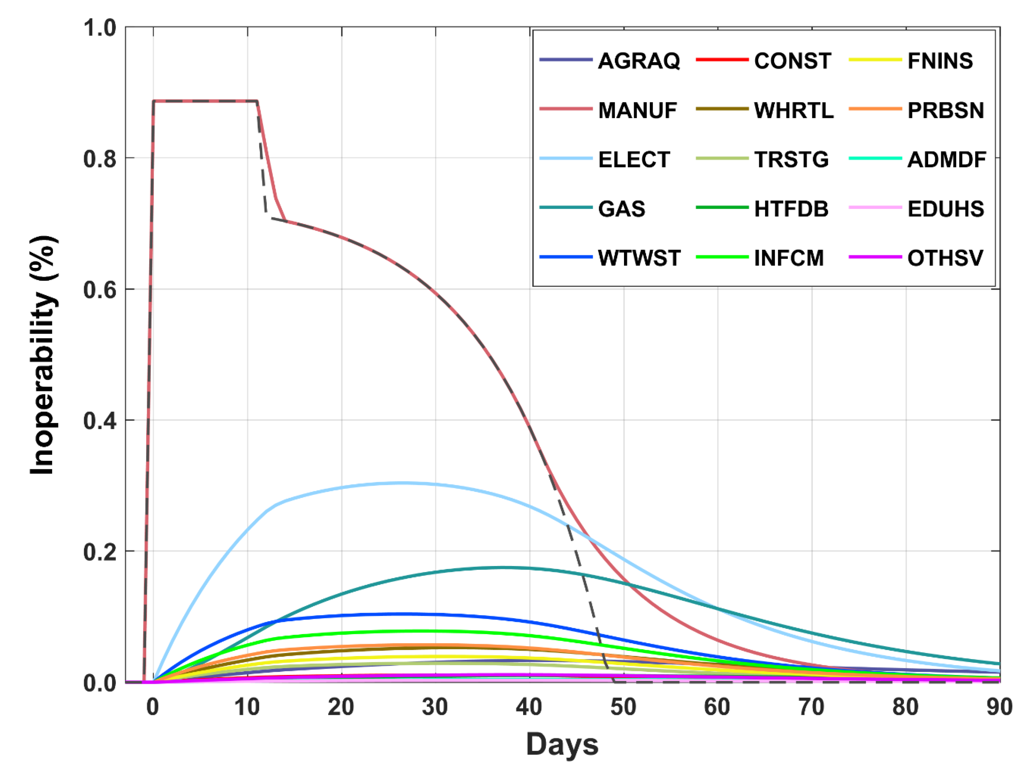
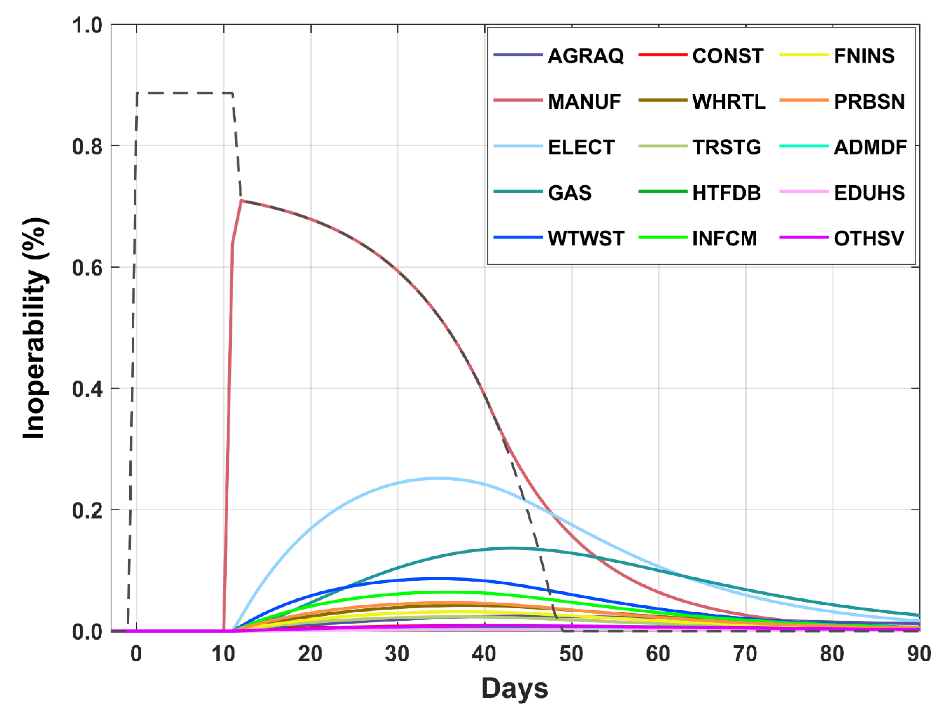
As in the previous section, the available inventory in each sector is assumed to be zero. The extended DIIM is then employed for the most likely recovery time vector T ´ and 1000 PERT-distributed T vectors to obtain corresponding inoperability trajectories. Figure 6 shows overall inoperability of each sector for the recovery time vector T ´ . Because of its slow initial recovery, p m a n u f t dominates the standard DIIM-based inoperability that includes interdependency effects, and thus determines the MANUF sector’s overall inoperability. A departure from this behavior is observed at t = 12 and 13 because of a sudden drop in p m a n u f t at t = 12. During the later stages (t > 42), the standard DIIM-based inoperability with its interdependency effect is larger than the rapidly decaying p m a n u f t and thus taken as the overall inoperability of the sector. Further, the overall inoperability trajectory follows the default concave-up exponential trajectory after deviating from p m a n u f t . The inoperabilities of indirectly affected sectors persist for a longer time compared to those in Section 5.2.1, thus resulting in larger average inoperability for each sector. Among the indirectly affected sectors, the ELECT sector has the largest q p followed by the GAS and WTWST sectors.
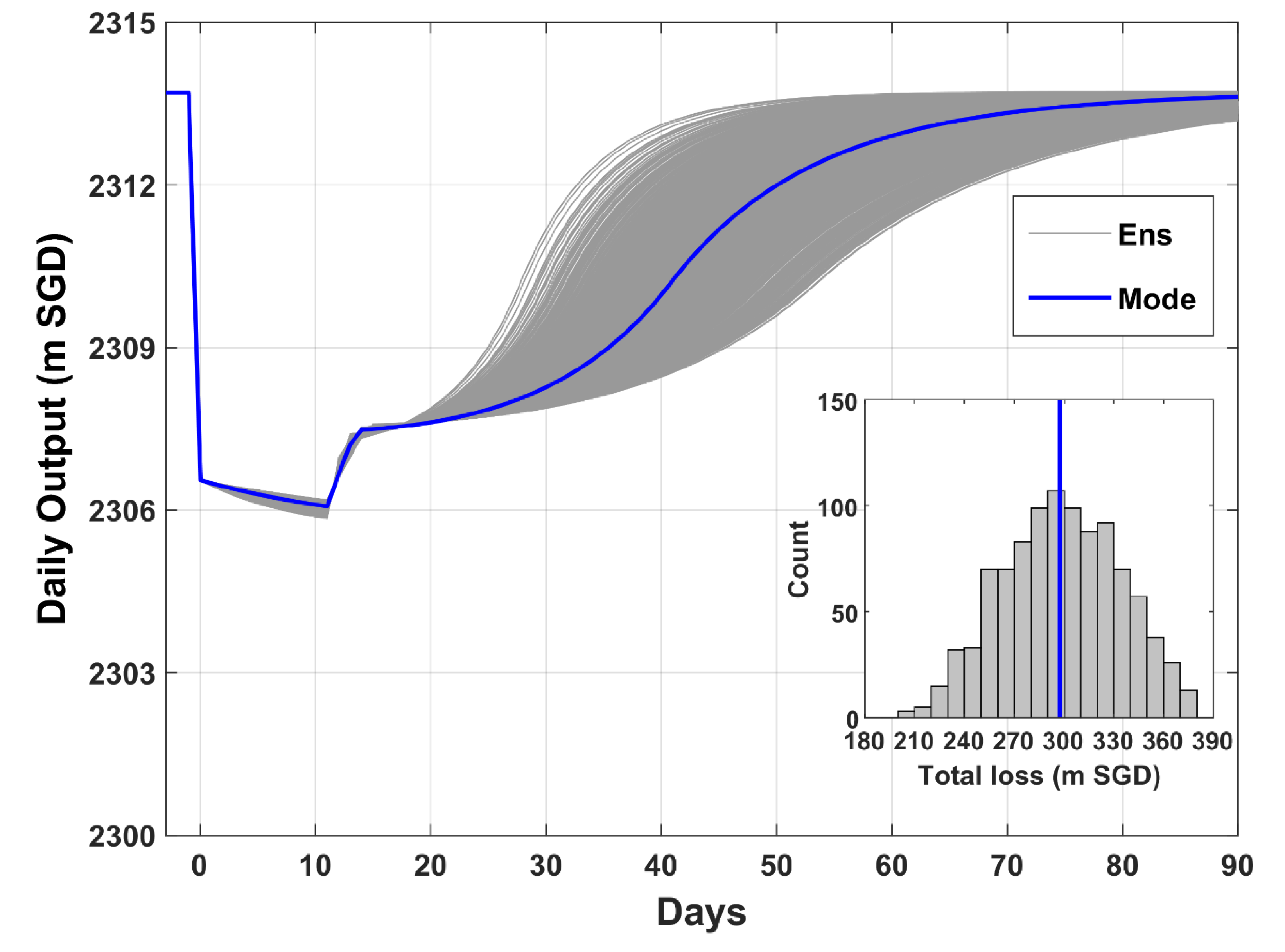
The inoperability trajectories are converted into daily economic output using Equation (8). The trajectories of total daily economic output for the most likely recovery time vector T ´ and for 1000 PERT-distributed T vectors are shown in Figure 7. Similar to Section 5.2.1, the daily economic output shows a slight decrease until t = 12 because of losses incurred by the indirectly affected sectors. From Day 13, the total output recovers following an s-shaped trajectory as a result of the MANUF sector’s concave-down overall inoperability during early stages and a concave-up inoperability in later stages. The impact of uncertain T on total output is greater for this scenario compared to the concave-up recovery scenario of Section 5.2.1, with the total loss ranging from $203.9 million to $375 million, and a value of $297.3 million for the most likely recovery time T ´ (Figure 7, inset). The total loss to the MANUF sector varies from $183–$336 million, with a value of $262 million for the recovery time vector T ´ .

5.2.3. Effect of Inventory

In Section 5.2.1 and Section 5.2.2, we assessed the impact of the PB fire for different production inoperability trajectories assuming no inventory. An inventory of finished goods if available at the time of a shock event can absorb the initial impact and consequently reduce higher-order losses. Therefore, holding an inventory of finished goods can be considered as a preparedness strategy to mitigate risk. Previous studies have used data on inventory-to-sales ratio to derive available inventory for affected sectors [32,46]). As this data is not publicly available for Singapore’s economic sectors, we assume that the MANUF sector has 10% of its output available as inventory at the time of PB fire. It is noted that according to the extended DIIM (Equation (6)), the inventory is used only for compensating the production inoperability of the directly affected sector, i.e., p m a n u f t .
The DIIM is then applied for the same concave-down p m a n u f t as in Section 5.2.2 but with an initial inventory in MANUF ( s m a n u f 0 ) set at 10% of the sector’s output. Figure 8 shows the sectoral inoperability curves for the recovery time vector T ´ . For the MANUF sector, s m a n u f 0 fully absorbs p m a n u f t until t = 10, and thus, according to Case 1 of Equation (6), the overall inoperability of the sector is same as the standard DIIM-based inoperability, which is zero as other sectors do not suffer any inoperability yet. The value of s m a n u f 0 depletes with time as it covers p m a n u f t , and, as a result, it can only partially absorb p m a n u f t at t = 11. The residual p m a n u f t of 0.64% is then the overall inoperability of the MANUF sector at t = 11 according to Case 2 of Equation (6). As inventory depletes to zero by t = 12, the overall inoperability of the MANUF sector traces the p m a n u f t trajectory following Case 3 of Equation (6). The MANUF inoperability then cascades to other sectors, among which the ELECT sector has the largest q p , followed by the GAS and WTWST sectors.
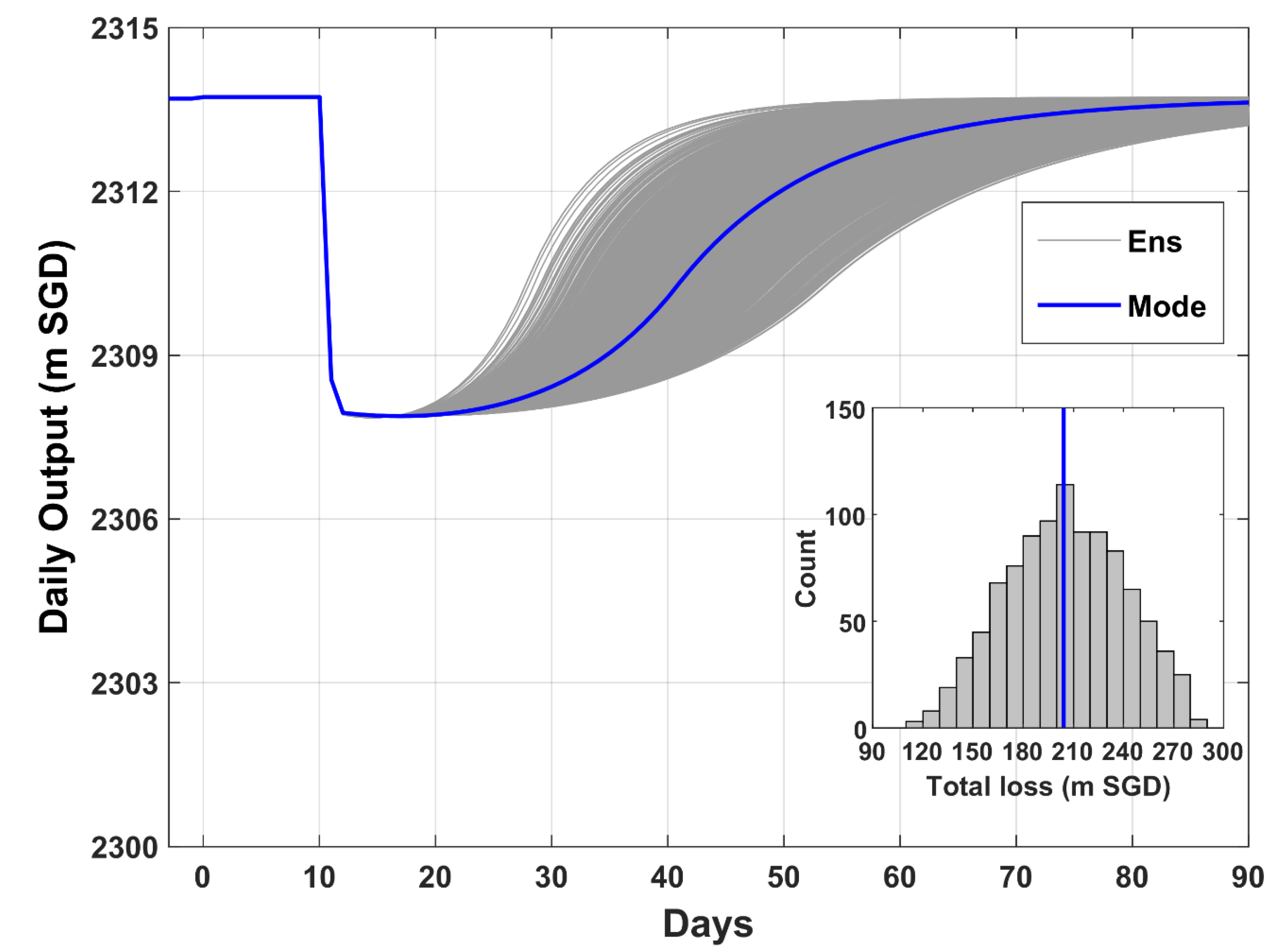
The total daily economic output trajectories for the most likely recovery time vector T ´ as well as 1000 PERT-distributed T vectors are shown in Figure 9. The daily output continues along the baseline economic output of $2313.7 million until t = 10 as the inventory fully covers the inoperability of the MANUF sector. From Day 12, the total output recovers following an s-shaped trajectory, similar to Section 5.2.2. The total loss ranges from $115.4 million to $283.1 million, with a value of $204.1 million for the most likely recovery time T ´ (Figure 9, inset). The corresponding total loss to the MANUF sector ranges from $101–$253 million, with a value of $180 million for the T ´ vector. Expectedly, the total loss is smaller than in the concave-down scenario with no inventory.
Royal Dutch Shell estimated a loss of $187 million to the company because of the PB refinery fire and the resulting shutdown [53]. As this loss value is exclusive to the company and not economy-wide, the MANUF sector’s predicted losses from our DIIM analysis should be comparable with this reported value. The losses to the MANUF sector for the most likely recovery time vector and for the three scenarios of concave up, concave down, and concave down with inventory, as assessed in Section 5.2.1, Section 5.2.2, and Section 5.2.3 are $161, $262, and $180 million, respectively. Together with the recovery time uncertainties, the full range of the MANUF sector’s losses is $101–$336 million and thus spans the reported loss of $187 million. Note that a more thorough evaluation of DIIM results is not conducted here as observational data on sectoral losses is not available.

5.3. Supply Side Inoperability IO Analysis

The models employed so far are driven by changes in final demand and/or production output via backward linkages with the upstream sectors [28,32]. Shock events also cause disruptions to the primary inputs which propagate downstream via forward linkages. Ghosh’s supply-side IO model, x = B · x + v or x = I B 1 v , where b i j B quantifies allocation of a unit output from sector i among all sectors j and v is a column vector of primary input, can obtain changes in output for exogenously specified changes in v [19,58]. However, the model has been criticized as “implausible”, with the main criticism being that it allows production increases in sectors without corresponding increases in their primary input use [59,60,61,62]. We acknowledge these arguments against the supply-side model and use the model in this study only for completeness. Further, we limit our analysis to the static version and interpret the results in terms of price changes instead of quantity changes as suggested by Dietzenbacher [63].
To be consistent with the rest of the study, we use the inoperability version of the supply-side IO model, which can be written as [64,65]:
q s = I A s * 1 v *
where A s * = x ^ 1 B x ^ = A T and v * = x ^ 1 Δ v is the normalized change in the primary input vector. The initial impact to the MANUF sector is entered into the model as a normalized change in primary input, v m a n u f * , calculated as Δ v m a n u f / x m a n u f = 0.0089 . The resulting sectoral inoperabilities obtained from supply-side IIM and the corresponding daily economic losses are shown in Table 2. Results reveal that the top three inoperable sectors besides the primarily affected MANUF sector are the CONST, HTFDB, and WTWST sectors. The top three indirectly affected sectors in terms of economic loss are the CONST, TRSTG, and PRBSN sectors.
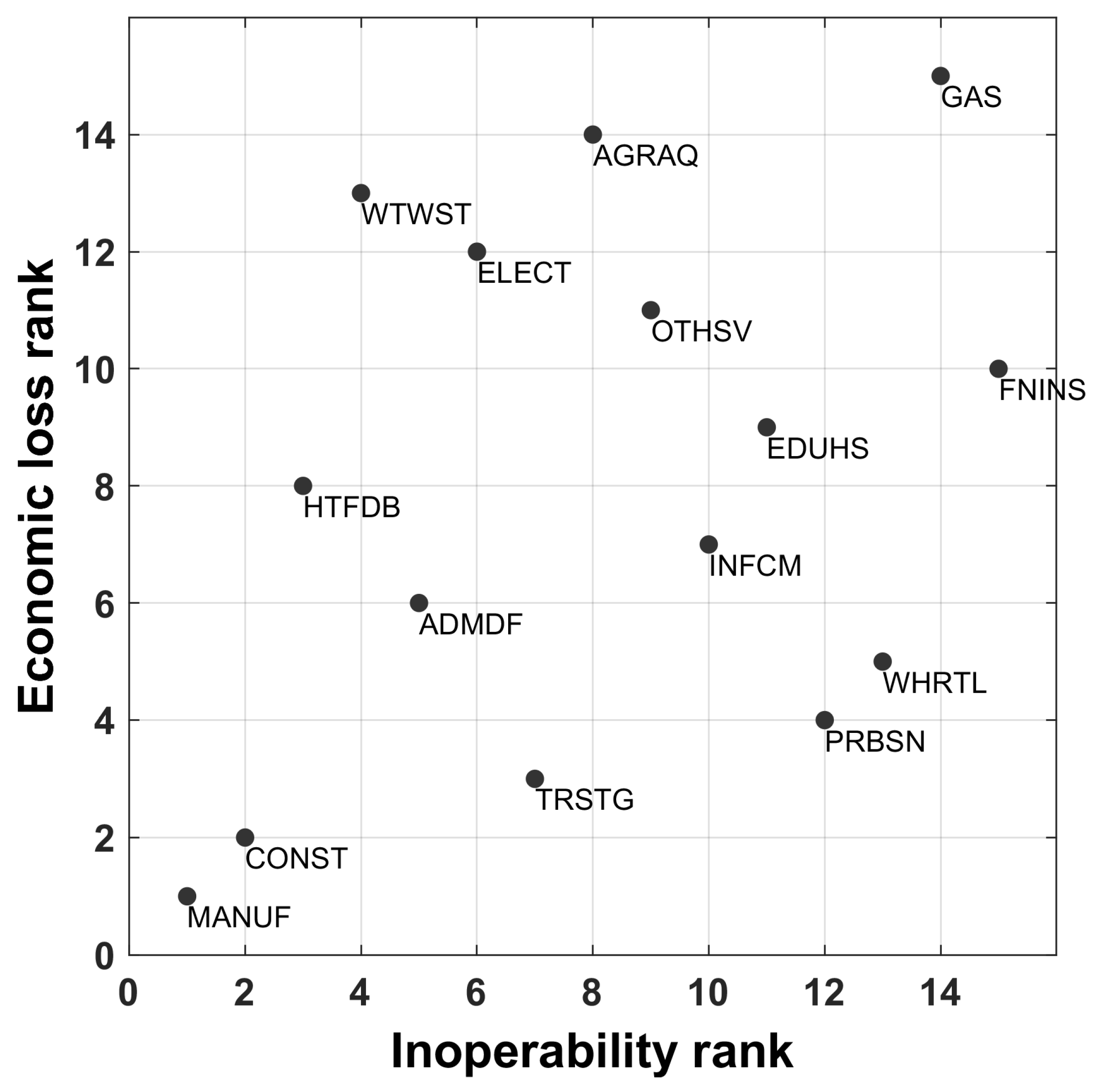
Figure 10 compares the sectors based on their inoperability and economic loss rankings. Besides the directly affected MANUF sector, the CONST sector ranks high both on inoperability and economic loss. The sectors HTFDB and WTWST rank high on the inoperability criterion, but, their economic output being smaller, rank low in terms of economic loss. Overall, the total daily loss due to the PB fire incident assessed via static supply-side IIM is $9.69 million. This value is interpreted here as the total loss due to an increase in the price of primary inputs. The total loss to the MANUF sector is $8.71 million or about 89.9% of the total loss. The higher-order losses are $9.69−$7.17 = $2.52 million, which are about 35% of the direct loss.

5.4. Linkage Analysis

The static IIM analyses showed that the higher-order loss due to the PB accident is ~38% of the direct loss for the demand-driven scenario (Section 5.1) and 35% for the supply-side scenario (Section 5.3). This can be explained from the perspective of the MANUF sector’s backward and forward linkages with all sectors of the economy including itself. Figure 11 shows the total backward and forward linkages obtained as column sums of the Leontief inverse I A 1 and row sums of the Ghosh inverse I B 1 , respectively. The backward linkage characterizes a sector’s connectivity with the upstream sectors from which it requires (purchases) inputs for production. The backward linkages obtained as above are the same as the simple output multipliers and quantify the total (direct + indirect) change in outputs from upstream sectors in response to a unit change in final demand for the sector’s output [19]. The MANUF sector’s backward linkage of 1.38 implies that the total demand-driven indirect losses throughout the economy are 38% of the direct losses to the sector. For a strongly backward-linked sector such as CONST, the total demand-driven indirect losses to the economy are about 102% of the direct loss to the sector.
The forward linkage characterizes a sector’s connectivity with downstream sectors to which it supplies (sells) its output and quantifies the total change in the value of outputs because of a unit change in the value of the primary inputs of the sector. Thus, the MANUF sector’s forward linkage of 1.35 implies that the total indirect losses are 35% of direct losses to the sector under the supply-side scenario. The utilities sectors (ELECT, GAS, WTWST) have stronger forward linkages, implying that a given direct loss when represented as the changes in primary inputs of these sectors leads to a larger percentage of indirect losses to the economy.
It is also observed in the static IIM analyses (Section 5.1 and Section 5.3) that a large part of the total loss, ~88% for the demand-driven and ~90% for the supply-side scenario, occurred in the MANUF sector. This is because the MANUF sector in Singapore, being highly import- and export-oriented, has weaker linkages with other sectors. Only 27% of the MANUF sector’s total inputs are from domestic industries, whereas 50% of inputs are imported (Figure 1). Similarly, only 25% of MANUF’s output is consumed by the domestic industries during the production process and 71% of output is exported. This can also be explained from Figure 11, which shows the top five backward- and forward-linked sectors for each sector. Every sector has a stronger linkage (both backward and forward) with itself followed by other sectors. However, the MANUF sector has the strongest self-linkage among all sectors, which explains why a large fraction of the total loss due to the PB fire accident is taken by the MANUF sector. For a sector such as ELECT, with its strong forward linkages with other sectors, the fraction of the total loss suffered by the ELECT sector under the supply-side scenario is about 49%, followed by about 26% by the MANUF sector.

6. Concluding Remarks

In this study, we have assessed the economic impacts of the PB refinery fire accident, considering interdependencies among 15 broadly grouped industrial sectors and using the inoperability IO models. For an initial impact of $7.17 SGD per day to the MANUF sector determined using the top-down approach, the indirect losses estimated using the static analyses were about 38% (35%) of the initial loss for the demand-driven (supply-side) scenario. A large fraction of the total loss was confined to the initially affected MANUF sector, with other sectors suffering about 10–12% of the total losses. The smaller indirect losses to other sectors were found to be because of weaker backward and forward linkages between the MANUF sector and other sectors of the economy. Among the indirectly affected sectors, WHRTL and PRBSN sectors suffered the most losses, whereas the utilities sectors such as ELECT and WTWST suffered the most inoperability.
The simulation experiments with DIIM and synthetic IO tables revealed that the recovery characteristics (duration and peak inoperability) of indirectly affected sectors are strongly tied to the recovery trajectory of the directly affected sector, e.g., faster recovery of a directly affected sector leads to faster recovery of an indirectly affected sector. Further, the simulation results showed that an indirectly affected sector has a higher peak inoperability when its recovery coefficient is larger, combined with a slower recovery of the directly affected sector. The DIIM analysis of the PB fire accident quantified the uncertainties in the recovery process; the total economic losses due to the PB fire range from $143–222 million for the concave-up (fast initial) recovery scenario, and from $204–375 million for the concave-down (slow initial) recovery scenario. On average, the losses from concave-down recovery were found to be about 1.6 times that of the concave-up scenario. It was also found that holding an inventory of about 10% of the MANUF sector can considerably absorb the initial impact, thus bringing the total losses in the range of $115–283 million.
This study focused on understanding the dynamics of recovery and indirect economic losses when the MANUF sector in Singapore is subjected to an initial impact. While the static and linkage analyses provided valuable insights into the initial vs. indirect losses for given sectoral interdependencies, the dynamic IIM proved to be a useful framework for incorporating the time-varying production inoperability of the initially affected sector and studying uncertainties in recovery scenarios and preparedness strategies. As earlier stated, this study assumed the initial impact of the PB refinery fire to be limited to the MANUF sector, and the production inoperabilities of other sectors were thus set to zero for the study time frame. Therefore, the cascading effects on other sectors are a result of the PB-fire-accident-driven inoperability in the MANUF sector. However, multiple shock events may occur in a short span of time and affect selected sectors in the same time frame. The DIIM model in this study can still be applied for such scenarios, though the multiple directly impacted sectors need to be identified and their production inoperability trajectories characterized using event-specific data. Thus, the DIIM model is readily extended to handle multiple directly impacted sectors, either from a single shock event or multiple events.
As IO models form the core of this study, the limitations of the IO framework, e.g., the linearity of production functions and the lack of substitution possibilities, apply to the current study as well. Further, the effects of shock-induced supply constraints were not explored in detail in this study. These limitations can be addressed to some extent by moving to hybrid models such as Adaptive Regional IO and non-linear programming models [21,66]. The current study is set in a single-region framework focusing on Singapore. Possible extensions of our work also include extending the analysis from a single-region framework to a multiregional one [67,68], considering the import and export dependencies between Singapore and other ASEAN countries.

Author Contributions

Conceptualization, P.V.M. and E.Y.M.L.; methodology, P.V.M. and E.Y.M.L.; software, P.V.M.; formal analysis, P.V.M.; investigation, P.V.M. and E.Y.M.L.; resources, E.Y.M.L.; data curation, P.V.M.; writing—original draft preparation, P.V.M.; writing—review and editing, P.V.M. and E.Y.M.L.; visualization, P.V.M..; supervision, E.Y.M.L.; project administration, E.Y.M.L.; funding acquisition, E.Y.M.L. All authors have read and agreed to the published version of the manuscript.

Funding

The research was conducted at the Future Resilient Systems of the Singapore-ETH Centre, which was established collaboratively between ETH Zurich and the National Research Foundation Singapore. This research is supported by the National Research Foundation Singapore (NRF) under its Campus for Research Excellence and Technological Enterprise (CREATE) programme.

Institutional Review Board Statement

Not applicable.

Informed Consent Statement

Not applicable.

Data Availability Statement

The datasets used in this study are procured from publicly available sources, whose links are provided in the references.

Conflicts of Interest

The authors declare no conflict of interest.

Appendix A

Table A1. List of 15 sectors used in this study and their corresponding subsectors from the official 105-sector Singapore IO table. The sector numbers in the third column are the same as in the official Singapore IO table.
Aggregated SectorsCodeComponent Sectors
Agriculture, livestock, and aquacultureAGRAQ1. Agriculture and nursery products, 2. Livestock, 3. Fishing and aquaculture
ManufacturingMANUF4. Food preparations, 5. Oils and fats, 6. Dairy products, 7. Other food products n.e.c., 8. Beverages and tobacco products, 9. Textiles, 10. Wearing apparel and fur products, 11. Footwear and leather products, 12. Wood and wooden products (except furniture), 13. Paper and paper products, 14. Printing and reproduction of recorded media, 15. Petroleum products, 16. Basic chemicals and chemical products, 17. Petrochemicals and petrochemical products, 18. Paints and related products, 19. Detergents, perfumes, cleaning and toilet preparations, 20. Other chemical products, 21. Pharmaceuticals and biological products, 22. Rubber and plastic products, 23. Other non-metallic mineral products, 24. Basic metals, 25. Fabricated metal products (except machinery and equipment), 26. Semiconductor devices, electronic components and boards, 27. Computers and peripheral equipment, 28. Communications equipment, 29. Consumer electronics, 30. Scientific, photographic and optical products, 31. Electrical industrial apparatus, batteries and accumulators, 32. Electric wiring and lighting equipment, 33. Domestic appliances, 34. Other electrical equipment, 35. General and special purpose machinery (except oil rigs), 36. Mining, quarrying and construction equipment, 37. Semiconductor related equipment, 38. Installation of industrial machinery and equipment, 39. Land transport equipment, 40. Ships and boats, 41. Aircraft and related parts, 42. Transport equipment n.e.c., 43. Furniture (except of stone), 44. Jewelry and related articles, 45. Medical and dental instruments and supplies, 46. Other manufacturing
ElectricityELECT47. Electricity
GasGAS48. Gas
Water and waste managementWTWST49. Water and sewerage, 50. Waste collection, treatment, and disposal services
ConstructionCONST51. Building construction, 52. Civil engineering works, 53. Specialized construction services
Wholesale and retailWHRTL54. Wholesale trade, 55. Retail trade
Transportation and storageTRSTG56. Land transport, 57. Water transport, 58. Air transport, 59. Land transport supporting services, 60. Water transport supporting services, 61. Air transport supporting services, 62. Cargo handling, warehousing, and other support services, 63. Postal and courier services
Hotels, food, and beverage servicesHTFDB64. Accommodation, 65. Food and beverage services
Information and communication servicesINFCM66. Publishing, 67. Media entertainment, 68. Telecommunications, 69. Computer programming, consultancy, and information services
Finance and insurance servicesFNINS70. Banking and finance, 71. Financial services (except insurance and pension funding), 72. Life insurance, 73. Non-life insurance, 74. Other auxiliary financial and insurance services, 75. Fund Management
Professional and business servicesPRBSN76. Real estate, 77. Ownership of dwellings, 78. Legal services, 79. Accounting, auditing, and tax consultancy services, 80. Head offices and business representative offices 81. Consultancy services, 82. Architectural and engineering services, 83. Research and development, 84. Advertising and market research, 85. Specialized design services, 86. Other professional, scientific and technical services, 87. Veterinary services, 88. Rental and leasing of tangible assets, 89. Rental and leasing of intangible assets, 90. Employment and labor contracting, 91. Travel agency, tour operator and reservation services, 92. Security and investigation services, 93. Cleaning and landscape maintenance services, 94. Office administrative and support services, 95. Exhibitions, conventions and other events
Public administration and defenseADMDF96. Public administration and defense services
Education, health. and social servicesEDUHS97. Education, 98. Health services, 99. Social services
Other servicesOTHSV100. Arts and entertainment, 101. Recreation and sports, 102. Member organizations, 103. Repair of computers, personal and household goods and vehicles, 104. Other personal services, 105. Domestic services

Appendix B

This appendix describes the simulation experiments to study the inoperability trajectory of an indirectly affected sector given an initial inoperability vector q 0 and the interdependency matrix A * . The simulations are conducted using synthetic two-sector and a five-sector IO tables.

Appendix B.1. Two-Sector IO Table

A * = 0.30 0.45 0.15 0.10
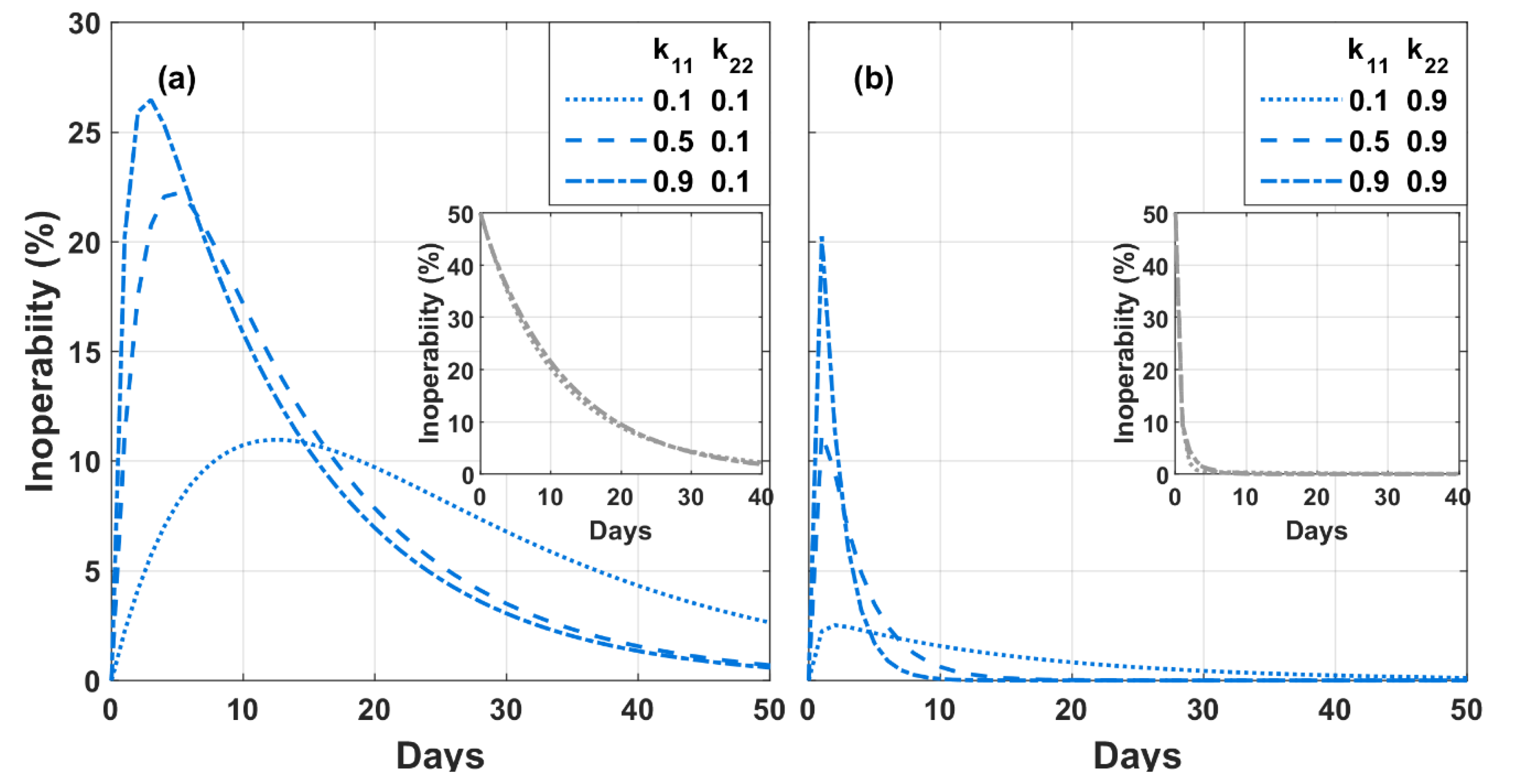
The initial inoperability vector for the two-sector experiment is assumed to be q 0 = 0.0   0.5 . Sector 2 is the directly affected sector with an initial inoperability of 50%. Two recovery coefficients are considered for Sector 2, i.e., k 22 = 0.1 or 0.9, while Sector 1’s k 11 is increased gradually as 0.1, 0.5, and 0.9, thus resulting in six combinations of k 11 , k 22 . Although Sector 1 has no initial inoperability, it is indirectly affected because of its dependence on Sector 2.
The sectoral inoperability trajectories for each k 11 , k 22 are obtained using the standard DIIM (Equation (3)) and shown in Figure A1. As the focus of the experiment is to understand the behaviour of an indirectly affected sector, Figure A1 highlights the trajectories of Sector 1, with the corresponding Sector 2 trajectories shown in the inset. It is observed that Sector 2’s trajectory is largely dependent on its own recovery coefficient k 22 , whereas Sector 1’s trajectory is sensitive to both k 11 and k 22 . Pant, et al. [69] illustrated using the same two-sector IO table that an indirectly affected sector recovers faster when both k 11 and k 22 are larger but such faster recovery comes at the cost of larger peak inoperability. This can be seen by comparing the trajectories of k 11 = 0.1 , k 22 = 0.1 (Figure A1a) and k 11 = 0.9 , k 22 = 0.9 (Figure A1b). Our simulations further reveal that for a fixed k 11 , Sector 1’s peak inoperability is larger when k 22 is smaller. The inoperability trajectory of an indirectly affected sector has a higher peak when its recovery coefficient is larger combined with a slower recovery of the directly affected sector.
Figure A1. Inoperability trajectories of the indirectly affected Sector 1 for three different recovery coefficients ( k 11 = 0.1, 0.5, 0.9) when the directly affected Sector 2’s recovery coefficient k 22 is (a) 0.1 and (b) 0.9. The inset in each panel shows the trajectories of the directly affected Sector 2 for each combination of k 11 , k 22 .
Sustainability 15 01739 g0a1

Appendix B.2. Five-Sector IO Table

A * = 0.050 0.167 0.083 0.100 0.150 0.100 0.050 0.075 0.025 0.275 0.140 0.160 0.080 0.060 0.240 0.050 0.125 0.150 0.050 0.175 0.160 0.060 0.200 0.100 0.040
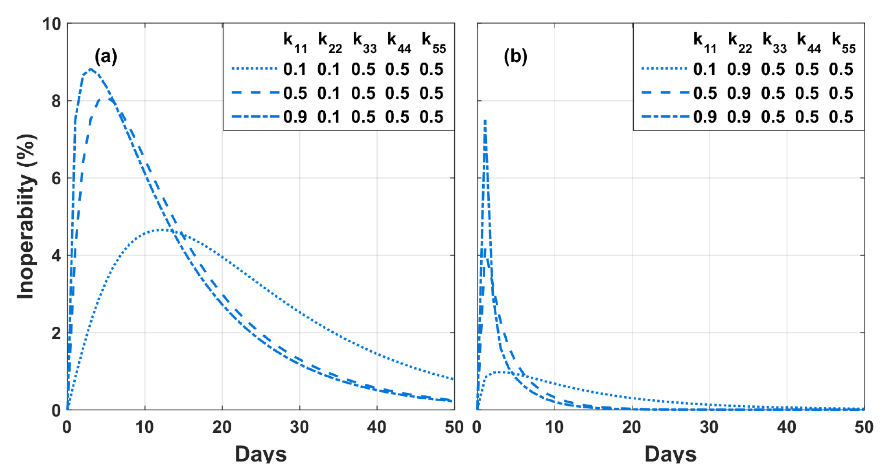
Similar to the two-sector experiment, Sector 2 is treated as the directly affected sector with an initial inoperability of 50%, i.e., q 0 = 0.0   0.5   0.0   0.0   0.0 . The recovery coefficient k 22 = 0.1 or 0.9, whereas k 11 is increased gradually from 0.1 to 0.5 and 0.9, keeping k 33 , k 44 , and k 55 fixed at 0.5. Figure A2 shows trajectories of Sector 1 for all six combinations of k 11 , k 22 , k 33 , k 44 , k 55 . Consistent with the results of the two-sector experiment, the peak inoperability of an indirectly affected sector is larger when its recovery coefficient is larger combined with a smaller recovery coefficient for the directly affected sector.
Figure A2. Inoperability trajectories of the indirectly affected Sector 1 for three different recovery coefficients ( k 11 = 0.1, 0.5, 0.9) when the directly affected Sector 2’s k 22 is (a) 0.1 and (b) 0.9. The recovery coefficients of Sectors 3, 4, and 5 are fixed at 0.5.
Sustainability 15 01739 g0a2
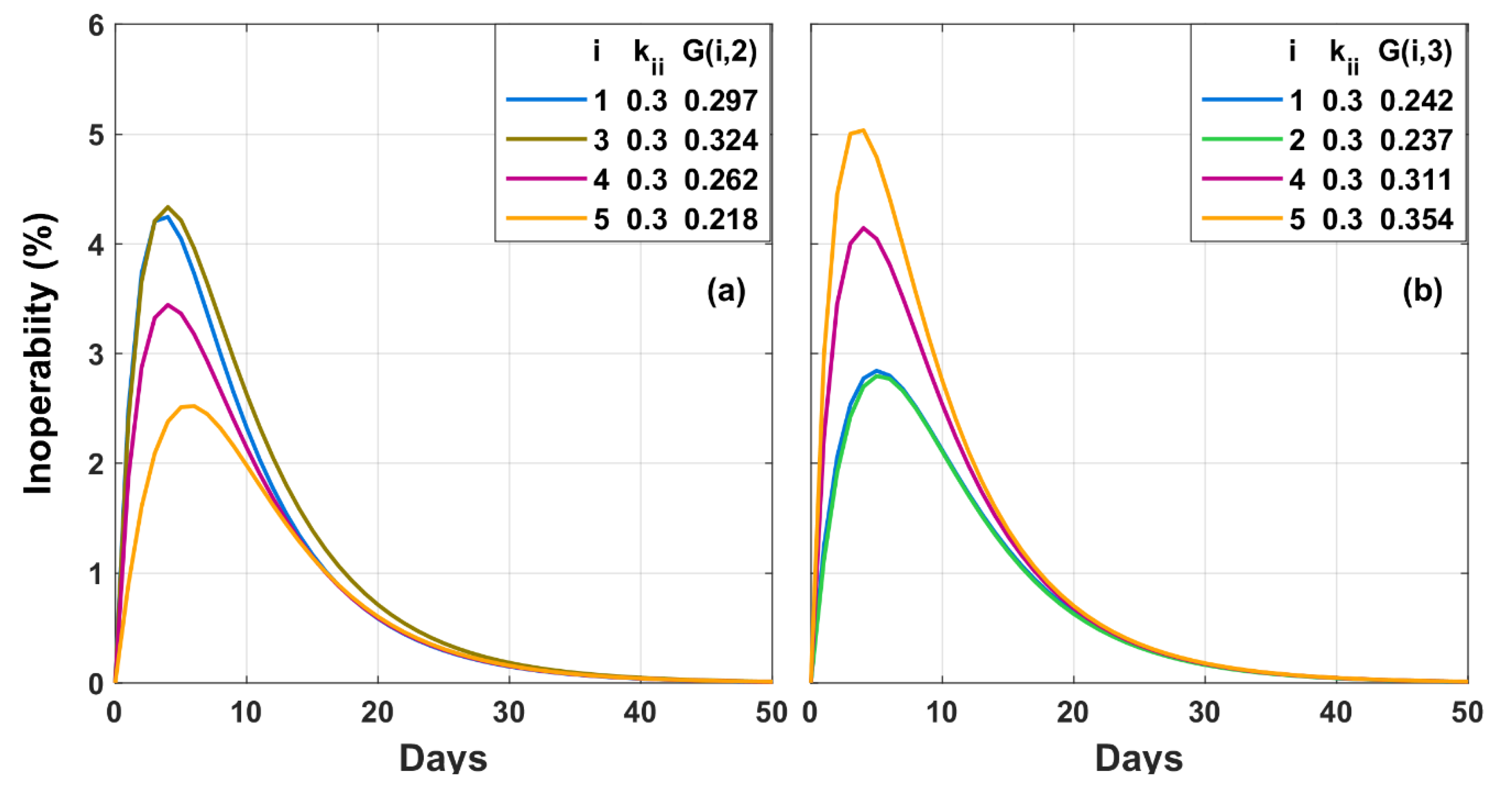
The five-sector IO table is also used to conduct an experiment where the recovery coefficient of each sector is fixed ( k i i = 0.3   i ). In such a scenario, for a directly affected sector j, the peak inoperability of an indirectly affected sector i (i     j) is mainly controlled by G i , j , where G = I A * 1 . The larger the G i , j , the higher the peak inoperability of the indirectly affected sector i (Figure A3).
Figure A3. Inoperability trajectories of all four indirectly affected sectors when the directly impacted sector is (a) Sector 2 and (b) Sector 3. The recovery coefficient is fixed at 0.3 for all sectors in both panels. The legend also shows the values of G i , j , where j is the directly affected sector and i is the indirectly affected sector.
Sustainability 15 01739 g0a3

References

  1. Rose, A.; Lim, D. Business interruption losses from natural hazards: Conceptual and methodological issues in the case of the Northridge earthquake. Glob. Environ. Change Part B Environ. Hazards 2002, 4, 1–14. [Google Scholar] [CrossRef]
  2. Hallegatte, S.; Przyluski, V. The Economics of Natural Disasters: Concepts and Methods; The World Bank: Washington, DC, USA, 2010. [Google Scholar]
  3. Meyer, V.; Becker, N.; Markantonis, V.; Schwarze, R.; van den Bergh, J.; Bouwer, L.M.; Bubeck, P.; Ciavola, P.; Genovese, E.; Green, C.; et al. Review article: Assessing the costs of natural hazards—State of the art and knowledge gaps. Nat. Hazards Earth Syst. Sci. 2013, 13, 1351–1373. [Google Scholar] [CrossRef] [Green Version]
  4. Hasan, S.; Foliente, G. Modeling infrastructure system interdependencies and socioeconomic impacts of failure in extreme events: Emerging R&D challenges. Nat. Hazards 2015, 78, 2143–2168. [Google Scholar] [CrossRef]
  5. Burrus, R.T., Jr.; Dumas, C.F.; Farrell, C.H.; Hall, W.W., Jr. Impact of low-intensity hurricanes on regional economic activity. Nat. Hazards Rev. 2002, 3, 118–125. [Google Scholar] [CrossRef]
  6. Anderson, C.W.; Santos, J.R.; Haimes, Y.Y. A risk-based input–output methodology for measuring the effects of the August 2003 northeast blackout. Econ. Syst. Res. 2007, 19, 183–204. [Google Scholar] [CrossRef]
  7. Kunz, M.; Muhr, B.; Kunz-Plapp, T.; Daniell, J.E.; Khazai, B.; Wenzel, F.; Vannieuwenhuyse, M.; Comes, T.; Elmer, F.; Schroter, K.; et al. Investigation of superstorm Sandy 2012 in a multi-disciplinary approach. Nat. Hazards Earth Syst. Sci. 2013, 13, 2579–2598. [Google Scholar] [CrossRef] [Green Version]
  8. Xia, Y.; Guan, D.B.; Steenge, A.E.; Dietzenbacher, E.; Meng, J.; Tinoco, D.M. Assessing the economic impacts of IT service shutdown during the York flood of 2015 in the UK. Proc. R. Soc. A-Math. Phys. Eng. Sci. 2019, 475. [Google Scholar] [CrossRef] [Green Version]
  9. Jin, X.; Sumaila, U.R.; Yin, K.D. Direct and Indirect Loss Evaluation of Storm Surge Disaster Based on Static and Dynamic Input-Output Models. Sustainability 2020, 12, 7347. [Google Scholar] [CrossRef]
  10. Chang, S.E.; Rose, A.Z. Towards a Theory of Economic Recovery from Disasters. Int. J. Mass Emergencies Disasters 2012, 30, 171–181. [Google Scholar] [CrossRef]
  11. Hallegatte, S. The Indirect Cost of Natural Disasters and an Economic Definition of Macroeconomic Resilience; The World Bank: Washington, DC, USA, 2015. [Google Scholar]
  12. Koks, E.E.; Carrera, L.; Jonkeren, O.; Aerts, J.; Husby, T.G.; Thissen, M.; Standardi, G.; Mysiak, J. Regional disaster impact analysis: Comparing input-output and computable general equilibrium models. Nat. Hazards Earth Syst. Sci. 2016, 16, 1911–1924. [Google Scholar] [CrossRef]
  13. Huang, R.; Malik, A.; Lenzen, M.; Jin, Y.T.; Wang, Y.F.; Faturay, F.; Zhu, Z.Y. Supply-chain impacts of Sichuan earthquake: A case study using disaster input-output analysis. Nat. Hazards 2022, 110, 2227–2248. [Google Scholar] [CrossRef]
  14. Ern, L.Y.; Abdullah, A. Fighting the shell pulau bukom fire: Strategies that worked for the SCDF. Home Team J. 2014, 2014, 66–73. [Google Scholar]
  15. Rose, A.; Liao, S.Y. Modeling regional economic resilience to disasters: A computable general equilibrium analysis of water service disruptions. J. Reg. Sci. 2005, 45, 75–112. [Google Scholar] [CrossRef]
  16. Hu, A.J.; Xie, W.; Li, N.; Xu, X.H.; Ji, Z.H.; Wu, J.D. Analyzing regional economic impact and resilience: A case study on electricity outages caused by the 2008 snowstorms in southern China. Nat. Hazards 2014, 70, 1019–1030. [Google Scholar] [CrossRef]
  17. Galbusera, L.; Giannopoulos, G. On input-output economic models in disaster impact assessment. Int. J. Disaster Risk Reduct. 2018, 30, 186–198. [Google Scholar] [CrossRef]
  18. Leontief, W. Input-Output Economics; Oxford University Press: Oxford, UK, 1986. [Google Scholar]
  19. Miller, R.E.; Blair, P.D. Input-Output Analysis: Foundations and Extensions; Cambridge University Press: Cambridge, UK, 2009. [Google Scholar]
  20. Okuyama, Y. Economic modeling for disaster impact analysis: Past, present, and future. Econ. Syst. Res. 2007, 19, 115–124. [Google Scholar] [CrossRef]
  21. Hallegatte, S. An adaptive regional input-output model and its application to the assessment of the economic cost of Katrina. Risk Anal. 2008, 28, 779–799. [Google Scholar] [CrossRef]
  22. Okuyama, Y.; Santos, J.R. Disaster impact and input–output analysis. Econ. Syst. Res. 2014, 26, 1–12. [Google Scholar] [CrossRef]
  23. Rose, A.; Guha, G.-S. Computable general equilibrium modeling of electric utility lifeline losses from earthquakes. In Modeling Spatial and Economic Impacts of Disasters; Springer: Berlin/Heidelberg, Germany, 2004; pp. 119–141. [Google Scholar]
  24. Tsuchiya, S.; Tatano, H.; Okada, N. Economic loss assessment due to railroad and highway disruptions. Econ. Syst. Res. 2007, 19, 147–162. [Google Scholar] [CrossRef]
  25. Zhou, L.; Chen, Z. Are CGE models reliable for disaster impact analyses? Econ. Syst. Res. 2021, 33, 20–46. [Google Scholar] [CrossRef]
  26. Rose, A. Economic principles, issues, and research priorities in hazard loss estimation. In Modeling Spatial and Economic Impacts of Disasters; Springer: Berlin/Heidelberg, Germany, 2004; pp. 13–36. [Google Scholar]
  27. Haimes, Y.Y.; Horowitz, B.M.; Lambert, J.H.; Santos, J.R.; Lian, C.Y.; Crowther, K.G. Inoperability Input-Output Model for Interdependent Infrastructure Sectors. I: Theory and Methodology. J. Infrastruct. Syst. 2005, 11, 67–79. [Google Scholar] [CrossRef]
  28. Lian, C.; Haimes, Y.Y. Managing the risk of terrorism to interdependent infrastructure systems through the dynamic inoperability input–output model. Syst. Eng. 2006, 9, 241–258. [Google Scholar] [CrossRef]
  29. Santos, J.R.; Orsi, M.J.; Bond, E.J. Pandemic Recovery Analysis Using the Dynamic Inoperability Input-Output Model. Risk Anal. 2009, 29, 1743–1758. [Google Scholar] [CrossRef] [PubMed]
  30. El Haimar, A.; Santos, J.R. Modeling Uncertainties in Workforce Disruptions from Influenza Pandemics Using Dynamic Input-Output Analysis. Risk Anal. 2014, 34, 401–415. [Google Scholar] [CrossRef] [PubMed]
  31. Khalid, M.A.; Ali, Y. Analysing economic impact on interdependent infrastructure after flood: Pakistan a case in point. Environ. Hazards-Hum. Policy Dimens. 2019, 18, 111–126. [Google Scholar] [CrossRef]
  32. Avelino, A.F.T.; Dall’erba, S. Comparing the Economic Impact of Natural Disasters Generated by Different Input-Output Models: An Application to the 2007 Chehalis River Flood (WA). Risk Anal. 2019, 39, 85–104. [Google Scholar] [CrossRef] [PubMed] [Green Version]
  33. Zhang, J.; Lu, M.; Zhang, L.L.; Xue, Y.D. Assessing indirect economic losses of landslides along highways. Nat. Hazards 2021, 106, 2775–2796. [Google Scholar] [CrossRef]
  34. Poudineh, R.; Jamasb, T. Electricity Supply Interruptions: Sectoral Interdependencies and the Cost of Energy Not Served for the Scottish Economy. Energy J. 2017, 38, 51–76. [Google Scholar] [CrossRef] [Green Version]
  35. Chen, H.; Yan, H.B.; Gong, K.; Geng, H.P.; Yuan, X.C. Assessing the business interruption costs from power outages in China. Energy Econ. 2022, 105. [Google Scholar] [CrossRef]
  36. Haimes, Y.Y.; Jiang, P. Leontief-based model of risk in complex interconnected infrastructures. J. Infrastruct. Syst. 2001, 7, 1–12. [Google Scholar] [CrossRef]
  37. Santos, J.R.; Haimes, Y.Y. Modeling the demand reduction input-output (I-O) inoperability due to terrorism of interconnected infrastructures. Risk Anal. 2004, 24, 1437–1451. [Google Scholar] [CrossRef]
  38. Crowther, K.G.; Haimes, Y.Y.; Taub, G. Systemic valuation of strategic preparedness through application of the inoperability input-output model with lessons learned from Hurricane Katrina. Risk Anal. 2007, 27, 1345–1364. [Google Scholar] [CrossRef] [PubMed]
  39. Dietzenbacher, E.; Miller, R.E. Reflections on the inoperability input–output model. Econ. Syst. Res. 2015, 27, 478–486. [Google Scholar] [CrossRef] [Green Version]
  40. Jonkeren, O.; Giannopoulos, G. Analysing Critical Infrastructure Failure with a Resilience Inoperability Input-Output Model. Econ. Syst. Res. 2014, 26, 39–59. [Google Scholar] [CrossRef]
  41. Vose, D. Risk Analysis: A Quantitative Guide; John Wiley & Sons: Hoboken, NJ, USA, 2008. [Google Scholar]
  42. Dahri, N.; Abida, H. Monte Carlo simulation-aided analytical hierarchy process (AHP) for flood susceptibility mapping in Gabes Basin (southeastern Tunisia). Environ. Earth Sci. 2017, 76, 302. [Google Scholar] [CrossRef]
  43. Benke, K.; Pelizaro, C. A spatial-statistical approach to the visualisation of uncertainty in land suitability analysis. J. Spat. Sci. 2010, 55, 257–272. [Google Scholar] [CrossRef]
  44. Xu, W.P.; Wang, Z.J.; Hong, L.; He, L.G.; Chen, X.G. The uncertainty recovery analysis for interdependent infrastructure systems using the dynamic inoperability input-output model. Int. J. Syst. Sci. 2015, 46, 1299–1306. [Google Scholar] [CrossRef]
  45. Jung, J.; Santos, J.R.; Haimes, Y.Y. International Trade Inoperability Input-Output Model (IT-IIM): Theory and Application. Risk Anal. 2009, 29, 137–154. [Google Scholar] [CrossRef]
  46. Barker, K.; Santos, J.R. Measuring the efficacy of inventory with a dynamic input-output model. Int. J. Prod. Econ. 2010, 126, 130–143. [Google Scholar] [CrossRef]
  47. Department of Statistics Singapore. National Accounts: Supply, Use and Input-Output Tables. Available online: https://www.singstat.gov.sg/find-data/search-by-theme/economy/national-accounts/latest-data#SU-IOT (accessed on 20 August 2022).
  48. Ng, W.H. Singapore, the Energy Economy: From the First Refinery to the End of Cheap Oil, 1960–2010; Routledge: Abingdon-on-Thames, UK, 2013. [Google Scholar]
  49. Chang, Y. Energy commodity trading in Singapore. In Energy Market Integration in East Asia: Energy Trade, Cross Border Electricity, and Price Mechanism; Han, P., Kimura, F., Eds.; ERIA Research Project Report FY2013; ERIA: Jakarta, Indonesia, 2014; pp. 13–26. [Google Scholar]
  50. British Petroleum, B. Statistical Review of World Energy 2021, 70th ed.; British Petroleum B: London, UK, 2021. [Google Scholar]
  51. ExxonMobil. Singapore Refinery. Available online: https://www.exxonmobil.com.sg/Company/Overview/Who-we-are/Singapore-Refinery (accessed on 26 August 2022).
  52. Lin, J.; Tai, K.; Tiong, R.L.K.; Sim, M.S. Analyzing Impact on Critical Infrastructure Using Input-Output Interdependency Model: Case Studies. Asce-Asme J. Risk Uncertain. Eng. Syst. Part A-Civ. Eng. 2017, 3, 04017016. [Google Scholar] [CrossRef]
  53. Chua, A. Pulau Bukom Fire. 2011. Available online: https://eresources.nlb.gov.sg/infopedia/articles/SIP_1868_2012-02-02.html (accessed on 20 August 2022).
  54. Ministry of Trade and Industry. 2nd Minister S Iswaran’s Reply on the Impact of the Shell oil Refinery Fire and Facilities Shut-down at Pulau Bukom on the Singapore Economy. Available online: https://www.mti.gov.sg/Newsroom/Parliamentary-Replies/2011/10/2nd-Minister-S-Iswarans-reply-to-Parliament-Question-on-the-impact-of-the-Shell-oil-refinery-fire-an (accessed on 20 August 2022).
  55. Department of Statistics Singapore. Share Of Nominal Gross Value Added, By Industry. SSIC. 2020. Available online: https://tablebuilder.singstat.gov.sg/table/TS/M015781 (accessed on 20 August 2022).
  56. Department of Statistics Singapore. Principal Statistics of Manufacturing by Industry Cluster-Value Added. Available online: https://tablebuilder.singstat.gov.sg/table/TS/M355181 (accessed on 20 August 2022).
  57. Haimes, Y.Y.; Horowitz, B.M.; Lambert, J.H.; Santos, J.; Crowther, K.; Lian, C.Y. Inoperability Input-Output Model for Interdependent Infrastructure Sectors. II: Case Studies. J. Infrastruct. Syst. 2005, 11, 80–92. [Google Scholar] [CrossRef]
  58. Ghosh, A. Input-output approach in an allocation system. Economica 1958, 25, 58–64. [Google Scholar] [CrossRef]
  59. Oosterhaven, J. On the plausibility of the supply-driven input-output model. J. Reg. Sci. 1988, 28, 203–217. [Google Scholar] [CrossRef]
  60. Oosterhaven, J. The supply-driven input-output model: A new interpretation but still implausible. J. Reg. Sci. 1989, 29, 459–465. [Google Scholar] [CrossRef]
  61. Gruver, G.W. On the Plausibility of the Supply—Driven Input-Output Model: A Theoretical Basis for Input-Coefficient Change. J. Reg. Sci. 1989, 29, 441–450. [Google Scholar] [CrossRef]
  62. De Mesnard, L. Is the Ghosh model interesting? J. Reg. Sci. 2009, 49, 361–372. [Google Scholar] [CrossRef]
  63. Dietzenbacher, E. In vindication of the Ghosh model: A reinterpretation as a price model. J. Reg. Sci. 1997, 37, 629–651. [Google Scholar] [CrossRef]
  64. Crowther, K.G.; Haimes, Y.Y. Application of the inoperability input—Output model (IIM) for systemic risk assessment and management of interdependent infrastructures. Syst. Eng. 2005, 8, 323–341. [Google Scholar] [CrossRef]
  65. Leung, M.; Haimes, Y.Y.; Santos, J.R. Supply- and Output-Side Extensions to the Inoperability Input-Output Model for Interdependent Infrastructures. J. Infrastruct. Syst. 2007, 13, 299–310. [Google Scholar] [CrossRef]
  66. Oosterhaven, J.; Bouwmeester, M.C. A new approach to modeling the impact of disruptive events. J. Reg. Sci. 2016, 56, 583–595. [Google Scholar] [CrossRef]
  67. Crowther, K.G.; Haimes, Y.Y. Development of the multiregional inoperability input-output model (MRIIM) for spatial explicitness in preparedness of interdependent regions. Syst. Eng. 2010, 13, 28–46. [Google Scholar] [CrossRef]
  68. MacKenzie, C.A.; Barker, K.; Grant, F.H. Evaluating the Consequences of an Inland Waterway Port Closure With a Dynamic Multiregional Interdependence Model. IEEE Trans. Syst. Man Cybern. Part A-Syst. Hum. 2012, 42, 359–370. [Google Scholar] [CrossRef]
  69. Pant, R.; Barker, K.; Zobel, C.W. Static and dynamic metrics of economic resilience for interdependent infrastructure and industry sectors. Reliab. Eng. Syst. Saf. 2014, 125, 92–102. [Google Scholar] [CrossRef]
Figure 1. Sectoral output (a), production cost (b), and use structure (c) in Singapore based on 2010 IO data.
Sustainability 15 01739 g001
Figure 2. Comparison of sector rankings derived based on economic loss and inoperability metrics.
Sustainability 15 01739 g002
Figure 3. Inoperability trajectory of each sector following the PB fire on Day 0. The dashed line depicts the production inoperability of the MANUF sector ( p m a n u f t from Equation (9)).
Sustainability 15 01739 g003
Figure 4. Peak inoperability of the indirectly affected sector i arranged in decreasing order, and the corresponding G i , M A N U F values plotted on the secondary y-axis.
Sustainability 15 01739 g004
Figure 5. Temporal evolution of the economic output for the most likely recovery time vector T ´ , and for each of 1000 T vectors (gray lines). The inset shows the histogram of total loss based on 1000 T vectors, with the solid blue line marking the loss for the most likely vector T ´ .
Sustainability 15 01739 g005
Figure 6. The inoperability trajectory of each sector due to the PB fire on Day 0. The dashed line depicts the production inoperability of the directly affected sector ( p m a n u f t from Equation (10)).
Sustainability 15 01739 g006
Figure 7. Temporal evolution of economic output for the most likely recovery time vector T ´ , and for each of 1000 T vectors (gray lines). The inset shows the histogram of total loss based on 1000 T vectors, with a solid blue line marking the loss for the most likely vector T ´ .
Sustainability 15 01739 g007
Figure 8. The inoperability trajectory of each sector due to the PB fire on Day 0. The dashed line depicts production inoperability of the directly affected sector ( p m a n u f t from Equation (10)).
Sustainability 15 01739 g008
Figure 9. Temporal evolution of economic output for the most likely recovery time vector T ´ , and for each of 1000 T vectors (gray lines). The inset shows the histogram of total loss based on 1000 T vectors, with the solid blue line marking the loss for the most likely vector T ´ .
Sustainability 15 01739 g009
Figure 10. Comparison of sector rankings derived based on economic loss and inoperability metrics for the supply-side IIM.
Sustainability 15 01739 g010
Figure 11. Total backward (a) and forward (b) linkages for 15 economic sectors in Singapore. The top five connected sectors for each sector are also shown.
Sustainability 15 01739 g011
Table 1. Sectoral inoperability and total daily economic loss because of PB fire- induced disruption to the final demand of the MANUF sector.
SectorInoperability
(%)
Total Daily Loss
(m SGD)
MANUF 1.088.71
ELECT 0.520.14
GAS 0.330.01
WTWST 0.180.02
INFCM 0.140.13
PRBSN 0.100.26
WHRTL 0.100.31
AGRAQ 0.090.00
FNINS 0.070.13
TRSTG 0.050.13
HTFDB 0.030.01
OTHSV 0.020.01
CONST 0.020.03
ADMDF 0.010.01
EDUHS 0.010.00
Please refer to Table A1 in Appendix A for details on sector abbreviations.
Table 2. Sectoral inoperability and total daily economic loss because of PB fire-induced disruption to the primary inputs of the MANUF sector.
SectorInoperability
(%)
Total Daily Loss
(m SGD)
MANUF1.088.71
CONST0.160.23
HTFDB0.130.05
WTWST0.120.01
ADMDF0.100.07
ELECT0.090.02
TRSTG0.080.20
AGRAQ0.070.00
OTHSV0.070.02
INFCM0.060.05
EDUHS0.060.04
PRBSN0.050.13
WHRTL0.040.11
GAS0.030.00
FNINS0.020.03
Please refer to Table A1 in Appendix A for details on sector abbreviations.
Disclaimer/Publisher’s Note: The statements, opinions and data contained in all publications are solely those of the individual author(s) and contributor(s) and not of MDPI and/or the editor(s). MDPI and/or the editor(s) disclaim responsibility for any injury to people or property resulting from any ideas, methods, instructions or products referred to in the content.