Article

Spatiotemporal Analysis of Future Trends in Terrestrial Water Storage Anomalies at Different Climatic Zones of India Using GRACE/GRACE-FO

by
Mohd Sayeed Ul Hasan
1,2,
Mufti Mohammad Saif
2,
Nehal Ahmad
2,
Abhishek Kumar Rai
1,
Mohammad Amir Khan
3,
Ali Aldrees
4,
Wahaj Ahmad Khan
5,
Mustafa K. A. Mohammed
6 and
Zaher Mundher Yaseen
7,8,*
1
Centre for Ocean, River, Atmosphere and Land Sciences, Indian Institute of Technology, Kharagpur 721302, India
2
Department of Civil Engineering, Aliah University, New Town 700160, India
3
Department of Civil Engineering, Galgotia College of Engineering, Knowledge Park I, Greater Noida 201310, India
4
Department of Civil Engineering, College of Engineering, Prince Sattam bin Abdulaziz University, Al-kharj 16273, Saudi Arabia
5
School of Civil Engineering & Architecture, Institute of Technology, Dire-Dawa University, Dire Dawa 1362, Ethiopia
6
Radiological Techniques Department, Al-Mustaqbal University College, Hillah 51001, Iraq
7
Civil and Environmental Engineering Department, King Fahd University of Petroleum & Minerals, Dhahran 31261, Saudi Arabia
8
Interdisciplinary Research Center for Membranes and Water Security, King Fahd University of Petroleum & Minerals, Dhahran 31261, Saudi Arabia
*
Author to whom correspondence should be addressed.
Sustainability 2023, 15(2), 1572; https://doi.org/10.3390/su15021572
Submission received: 21 November 2022 / Revised: 29 December 2022 / Accepted: 9 January 2023 / Published: 13 January 2023

Abstract

:
This work is a climatological evaluation of terrestrial water storage anomalies (TWSAs), which act as driving forces for sustainable development, in one of the most populous countries of the world. The objective of this work is to evaluate RL06 mascon data from the GRACE and GRACE-FO satellite missions over India to explore seasonal and interannual changes in terrestrial water storage, encompassing an area of ~3.29 million km2 with 285 grid points, from 2002 through to 2020. Several statistical tests are performed to check the homogeneity (i.e., Pettitt’s test, the BRT, the SNHT, and the VNRT). Most of the homogeneous data are found in winter, pre-monsoon, and post-monsoon, approximately above 42% to 47%, and the least are found in monsoons and annual with only 33%, at a 95% significance level. According to Pettitt’s test, the majority of the breakpoints are present in 2014 for winter, 2012 for pre-monsoon, 2011 for monsoons and post-monsoon, and 2008 as well as 2011 for annual. Furthermore, to detect trends and magnitudes we employed the nonparametric MK test, the MMK test, Sen’s slope estimator, and the parametric SLR test. According to the MK and MMK tests, the most significant negative and positive trends indicate the chances of droughts and floods, respectively. The Indo–Gangetic region shows the highest declination. According to Sen’s slope and the SLR test, the most declining magnitude is found in Delhi, Panjab, Uttrakhand, the northern part of Rajasthan, and Uttar Pradesh. Based on our findings, the average declining rate of yearly terrestrial water storage data from the MK, MMK, and SLR tests is −0.0075 m (−0.75 cm/year) from 2002 to 2020. Koppen–Geiger climate zones are also used to depict the seasonal and interannual descriptive statistics of TWSA trends. Interestingly, the annual means of arid desert cold (−0.1788 cm/year) and tropical savanna (−0.1936 cm/year) have the smallest declining trends when compared to other climatic zones. Northern Indian regions’ temperate dry winter, hot/warm summer, and dry arid steppe hot regions show the maximum declining future trend. This study could be useful in planning and managing water resources, agriculture, and the long-term growth of the country by using an intelligent water delivery system.

1. Introduction

Terrestrial water storage (TWS) refers to all physical phases of water held above and below the Earth’s surface, such as soil moisture, snow, ice, canopy water storage, groundwater, and so on [1]. As an important component of terrestrial and global hydrological cycles, TWS has a considerable influence on water, energy, and biogeochemical fluxes, and hence plays a significant role in Earth’s climate system [2,3]. Within a region or basin, TWS plays a key role in maintaining the hydrological equilibrium (P = R + ET + TWSC) because evapotranspiration (ET), runoff (R), and changes in TWS are all connected [1]. According to the authors of [4,5], TWS has significant implications for water resource management and long-term utilization. Additionally, TWS variations have a large impact on terrestrial ecosystems, humans, and even sea levels [6]. Monitoring variations in TWS can help manage water in India, which is already under pressure due to increased water consumption in agriculture, households, and industries, in addition to climate change [7].
TWSA became more helpful in hydrological studies after 2002, when reliable estimates became available from the Gravity Recovery and Climate Experiment (GRACE) satellite, which was introduced by the National Aeronautics and Space Administration (NASA) and the German Aerospace Center (DLR) [7]. GRACE provides an advantage over traditional remote sensing and ungauged catchment measurements in that it can discern more nuances in the total amount of water stored from the surface to the deepest aquifer, including groundwater [7]. Furthermore, GRACE observations have also demonstrated great potential for predicting groundwater depletion [8,9,10] and exploring climate–human interactions [11]. To continue measuring the Earth’s gravity field, the GRACE joint project was renamed as the Gravity Recovery and Climate Experiment Follow-On (GRACE-FO) in May 2018.
Changes in TWSAs have also been affected by the gradual decline in groundwater since the rapid industrialization and population growth of the 21st century [12]. Due to groundwater depletion, the decline in groundwater storage, i.e., the sustainability of water supplies, is considered a global problem [13]. Groundwater is the most important component of terrestrial water storage, and human civilization’s expansion and survival are largely dependent on it. In India, for Rajasthan, Punjab, Haryana, and Delhi, the entire groundwater depletion from August 2002 to October 2008 for these locations was equivalent to 109 km3 of water, and the depletion rate was 4.0 ± 1.0 cm/year [14,15]. According to the authors of [16], the groundwater levels in large locations in India have dropped significantly from 1980 to 2010, ranging from 4 m to 16 m. Aside from irrigation, urbanization and climate change both have a major impact on groundwater storage [17]. In the past decade there has been a significant decrease in groundwater levels: around 65% of Indian wells showed a decrease in groundwater levels between 2006 and 2016 [18].
In this study, the homogeneity test is used to calculate the data variability and the nature of the distribution. Homogeneous data are obtained when measurements are made at the same time with the same spatial location and in the environment. However, dealing with terrestrial water storage anomaly data is difficult since the data are constantly influenced by changes in measurement techniques and procedures, environmental characteristics and structures, and spatial locations. Pettitt’s test [19], the standard normal homogeneity test (SNHT) [20], the Buishand range test (BRT) [21], and the von Neumann ratio test (VNRT) [22] are the most frequently and extensively suggested methods for detecting the nature of homogeneity in time series [23]. These four tests were applied to the European climate by Wijngaard [24]. The results are divided into three categories based on the number of tests that reject the null hypothesis (alpha of 0.05) at a significance of 95%: homogeneous or useful, doubtful, and suspect or inhomogeneous. Their study found that homogeneity analyses are largely dependent on the test variables, test procedures, and significance levels employed [25,26,27,28,29,30]. In addition, their research on climate series demonstrates the importance of statistical analyses in determining homogeneity and trends [31]. In our study, Pettitt’s test, the standard normal homogeneity test (SNHT), the Buishand range test (BRT), and von Neumann’s test are used to detect the monthly terrestrial water storage data of 285 grid points from 2002 to 2020 on seasonal and annual bases in India.
The mascons recently represented an alternative method with which to produce thorough TWSA calculations. The benefits of utilizing mascons include keeping an enhanced gravity signal using position data, lowering residual noise, and minimizing spatial leakage errors. The mascon solutions could typically be employed directly without the need for scaling factors or other post-processing techniques [32]. A number of separate releases (RL)—RL04, RL05, and RL06—have been produced as a result of the numerous revisions and improvements that each of these solutions have been through. With each new release, GRACE products have become better than their predecessors [33]. The climatological variability of TWSAs is also analyzed by a globally accepted nonparametric trend test to identify the nature and magnitude of the trend using the Mann–Kendall (MK) test, the modified Mann–Kendall (MMK) test, Sen’s slope estimator (SS), and the parametric test by simple linear regression analysis (SLRA) [26,29,34]. The long-term trends in India’s winter (post-monsoon Rabi), pre-monsoon, monsoon, post-monsoon Kharif, and annual terrestrial water storage data are examined by using the MK, MMK, SLR, and SS tests over a span of 19 years, and obvious trends are also reported in the different climatic regions.

2. Study Area and Data Resources

2.1. Study Area

India is the world’s seventh-largest country, with 2.28% (297 million hectares) of the world’s global territory and 17.8% (1.24 billion) of its population in 2011 [35]. India’s latitudes and longitudes range from 8°4′ north to 37°6′ north, and from 68°7′ east to 97°25′ east, respectively (Figure 1). The Himalayas and related mountains, Indo–Gangetic plain, and peninsular shield are the three major geological regions of India [36], which are separated into six zones: the northern zone, central zone, eastern zone, western zone, southern zone, and northeastern zone. The climate in India is predominantly tropical monsoon, with maximum average temperatures ranging from 24.5 °C in winter to 31.5 °C in summer and minimum average temperatures ranging from 13.85 °C in winter to 23.27 °C in a monsoon. The average rainfall in India varies from 41.87 mm in winter to 887.48 mm during a monsoon. The GRACE data included 285 grid points in India from various geographic regions to investigate the terrestrial water storage conditions, and we observe each grid point separately to avoid inter-relationships.
The total groundwater withdrawals in 2011 were approximately 245 billion cubic meters, placing it first on the utilization list [37]. The use of groundwater for agriculture accounts for more than 90% of total groundwater resources [38]. In our study area, the monthly TWS data are classified into four seasons according to Indian Metrological Department (IMD) classifications. These are winter (post-monsoon Rabi) (January to March), summer (pre-monsoon) (April to June), monsoon (July to September), and post-monsoon Kharif (October to December).

2.2. Data Source: GRACE-Derived TWSAs

NASA and the German Aerospace Center, Deutscen Für Luftund Raumfahrt (DLR), launched the Gravity Recovery and Climate Experiment (GRACE) satellite mission in March 2002 to research the Earth’s gravitational field on a monthly basis. The GRACE Follow-On (GRACE-FO) mission, which was launched on 22 May 2018, is GRACE’s successor, while there are time gaps between GRACE and GRACE-FO. Here, in this study, linear interpolation is used to fill in the missing months’ data. The twin satellites’ distance is affected by the Earth’s gravitational field’s spatial and temporal fluctuations. These variations can be used to monitor hydrological signals in the form of changes in terrestrial water on a monthly basis [39,40].
In this study, the analysis is based on the most recent GRACE monthly mass grids (RL 06) processed at the Jet Propulsion Laboratory (JPL) https://grace.jpl.nasa.gov (accessed on 1 September 2021). These monthly TWSA data from 2002 to 2020, with a spatial resolution of 1° × 1°, are processed and analyzed on a seasonal basis. Furthermore, all of the 285 grid points’ seasonal and annual data are imported into the GIS platform for an additional inverse distance weightage (IDW) analysis to generate the surface raster [41]. Another advantage of RL06 is that, over coastlines, the signal leakage errors are decreased by the coastal resolution improvement (CRI) filter to improve the data accuracy of GRACE TWSAs [42]. Geographic maps representing data changes across time, both seasonal and annual, are created using the IDW interpolation approach.

3. Modeling Results

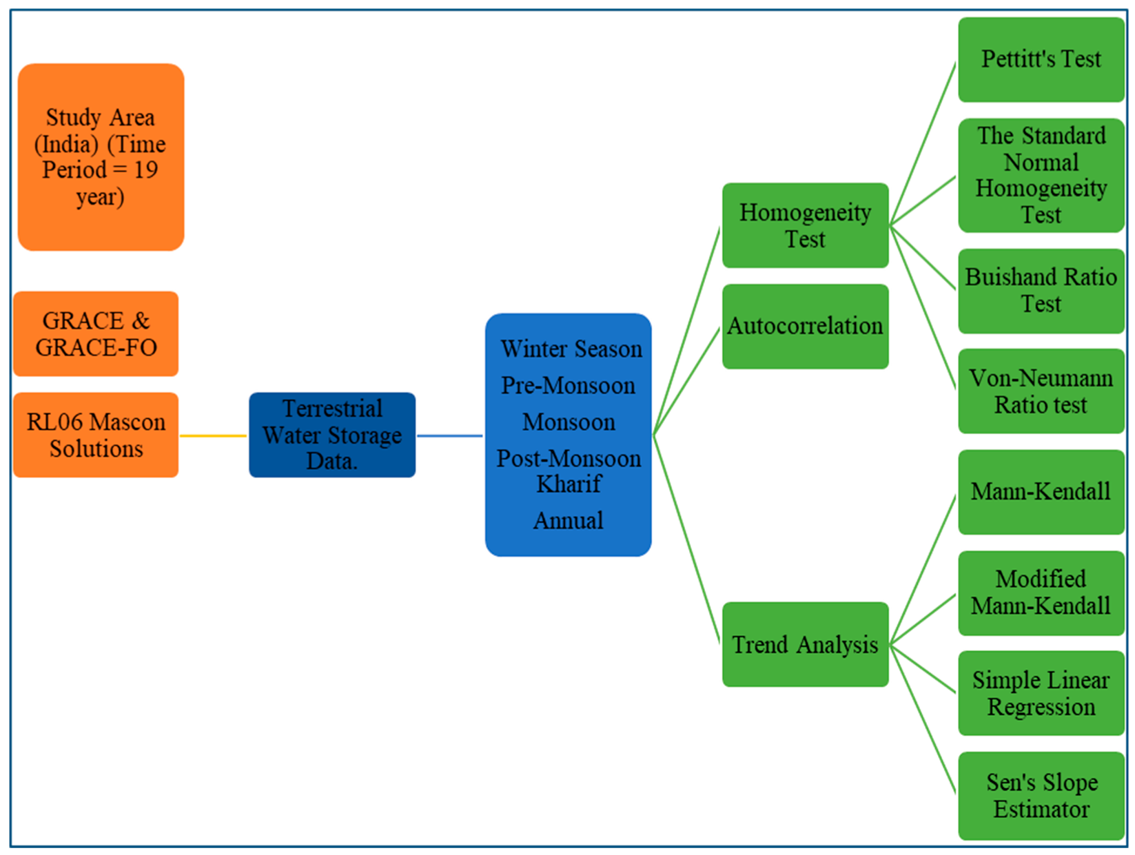
In this study, we analyzed the monthly terrestrial water storage data of 285 grid points, from 2002 to 2020, on seasonal and annual bases. We used four methods (at a 95% significant level) to check the homogeneity of the data and the results are shown below. In addition, we used parametric and nonparametric tests to examine the trends (Figure 2).

3.1. Seasonal Homogeneity Test Results

3.1.1. Winter Season

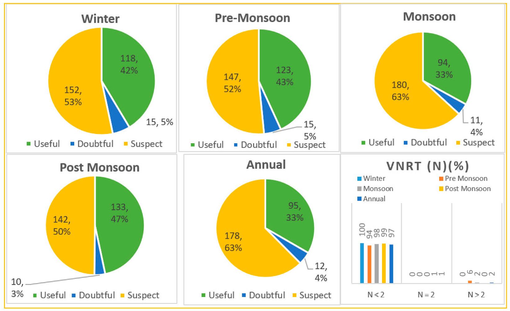
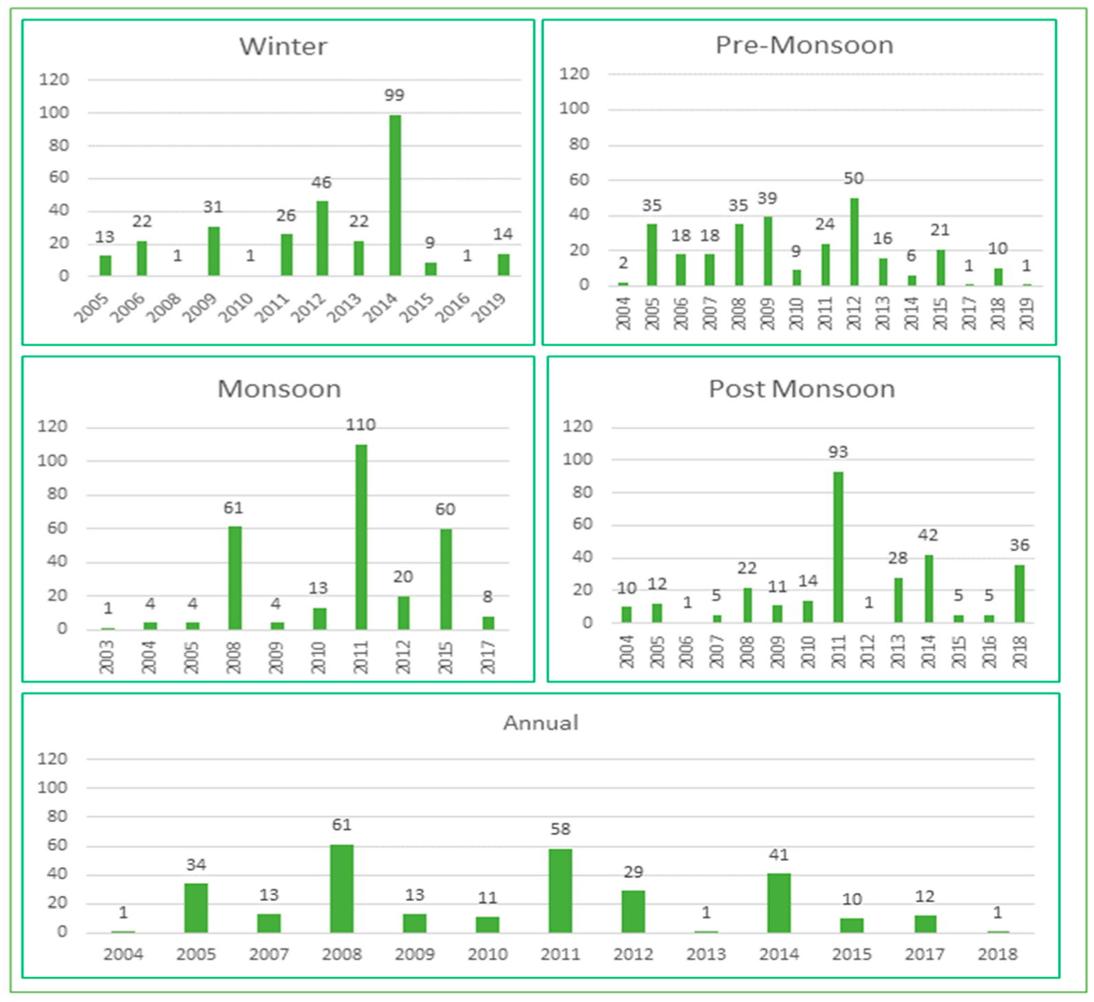
In India, the winter season (post-monsoon Rabi) is defined as being January through to March, according to the IMD categorization. During the winter season, four homogeneity test methods are used to test the 285-grid-point data of terrestrial water storage from 2002 to 2020. According to a p-value with a 95% significant level, compared with an alpha of 0.05, the four tests are characterized as useful, doubtful, and suspect; based on this, the results are 42% (118 grid points), 5% (15 grid points), and 53% (152 grid points), respectively, and these are also shown in Figure 3. During the winter season, in the VNR test, all values of the von Neumann ratio (N) < 2 refer to the fact that change points are present in all of the data (Figure 3). The values range from 0.0931 (longitude of 78.5, latitude of 29.5) to 1.6891 (longitude of 78.5, latitude of 29.5) (longitude of 80.5, latitude of 22.5). According to Pettitt’s test, the majority of the breakpoints occurred in 2014, and these are shown in Figure 4 and Figure 5.

3.1.2. Pre-Monsoon Season

Pre-monsoon is defined as the period between April and June, according to the IMD classification. According to the classification of useful, doubtful, and suspect, the results are 43% (123 grid points), 5% (15 grid points), and 52% (147 grid points), respectively, and these are also shown in Figure 3.
In the VNR test, the observed value of N < 2 is 94% (268 grid points) in these data where change points are present. The values vary from 0.1607 (longitude of 75.5, latitude of 28.5) to 1.9826 (longitude of 80.5, latitude of 21.5). Here, only a grid point (longitude of 78.5, latitude of 23.5) where N = 2 means that, at this point, the data are deemed homogeneous, and only 6% (16 grid locations) becomes N > 2; this grid represents rapid variations in the mean. The VNR (N) ranges from 2.1217 (longitude of 79.5, latitude of 23.5) to 2.2065 (longitude of 79.5, latitude of 23.5) (longitude of 86.5, latitude of 20.5). According to Pettitt’s test, the majority of the breakpoints are shown as being in 2008 and 2012 (Figure 4 and Figure 5).

3.1.3. Monsoon Season

According to the IMD classification, July through to September represents the monsoon season. In the monsoon season, according to a p-value at a 95% significance level, the terrestrial water storage data of 285 grid points are categorized as useful, 33% (94 grid points), doubtful, 4% (11 grid points), and suspect, 63% (180 grid points), by four homogeneity test methods.
Here, in the VNR test, 98% (280 grid points) of data where N < 2 represents most of the data where change points are present. These data range from 0.1880 (longitude of 76.5, latitude of 28.5) to 1.9356 (longitude of 74.5, latitude of 35.5). According to Pettitt’s test, the majority of the breakpoints are shown as being in 2011 and 2015, and this variation is shown in Figure 4 and Figure 5.

3.1.4. Post-Monsoon Season

As per the IMD classification, October to December is called the post-monsoon season. Here, we also calculated the 285-grid-point data of terrestrial water storage, and the results suggested by the four homogeneity tests with a 95% significant level of the p-value results are as follows: 47% (133 grid points), 3% (10 grid points), and 50% (142 grid points) categorized as useful, doubtful, and suspect, respectively, also shown in Figure 3. In the VNRT, the observed values where N tended to be < 2 were 99% (282 grid points), which is why most of the data had change points present. The values vary from 0.1241 (longitude of 77.5, latitude of 29.5) to 1.9569 (longitude of 79.5, latitude of 23.5). Additionally, it is observed that N = 2 only one value in (longitude of 78.5, latitude of 23.5), and the series is considered homogenous. Of the grid points, 1% (two grid points) becomes N > 2 in these two grids, representing rapid variations in the mean, shown in Figure 3. The values were 2.0131 (longitude of 76.5, latitude of 9.5) and 2.370 (longitude of 77.5, latitude of 8.5). All of the homogeneity tests, except VNR, indicate that most of the breakpoints were detected in 2011, 2014, and 2018, and others are shown in Figure 4 and Figure 5.

3.1.5. Annual Mean

All of the seasonal data will be analyzed every year to determine the annual changes in TWS at various grid locations. We compared the data using an alpha value of 0.05 to see if there was any homogeneity. According to the four techniques, 33% (95 grid points) of the yearly terrestrial water storage data is “useful”, just 4% (12 grid points) is “doubtful”, and 63% (178 grid points) is “suspect” (Figure 3). Thus, 285 grid points with homogeneous data were chosen for further trend analyses.
The observed value of N < 2 in the VNRT is 97% (278 grid points), which explains why the majority of the data had change points (Figure 3). The number ranges from 0.0946 (longitude of 76.5, latitude of 28.5) to 1.8680 (longitude of 76.5, latitude of 28.5) (longitude of 74.5, latitude of 34.5). The data where N = 2 only have two values (longitude of 74.5, latitude of 35.5) (longitude of 75.5, latitude of 35.5). The five grid points’ values vary from 2.0215 (longitude of 74.5, latitude of 34.5) to 2.2498 (longitude of 74.5, latitude of 34.5), where N > 2 demonstrates rapid fluctuations in the mean. Except for the VNRT, all of the homogeneity tests show that the majority of the breakpoint were detected in 2008 and 2012 (Figure 4 and Figure 5).

3.2. Trend Analysis

3.2.1. Winter Season

Autocorrelation: In the winter season, we analyzed 285 grid points of terrestrial water storage data from 2002 to 2020 using autocorrelation at a significance level of 95%. The results show 40% (115 grid points) with p > 0.05 and 60% (170 grid points) with p < 0.05, with values ranging from 0.0002 to 0.9183.
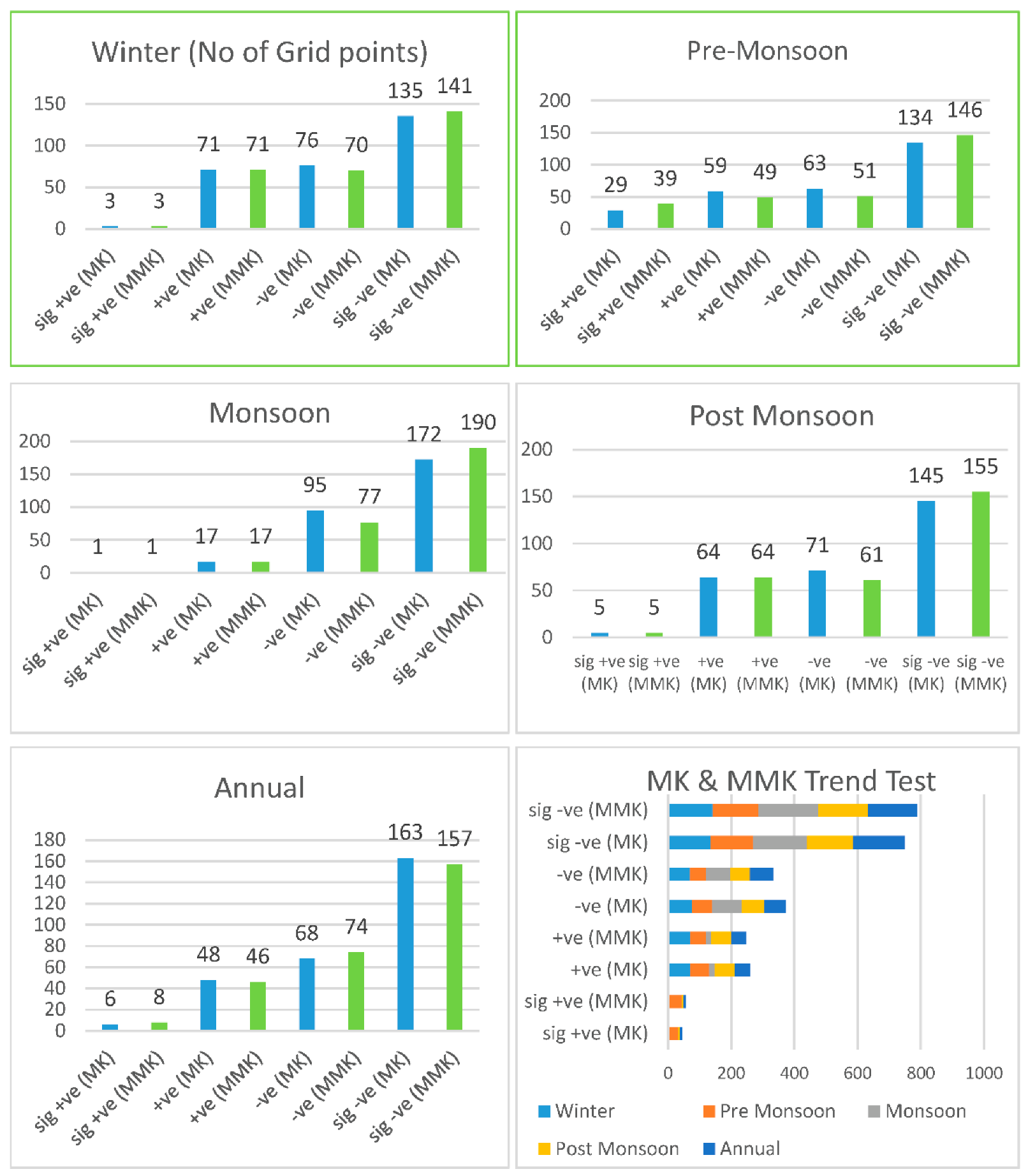
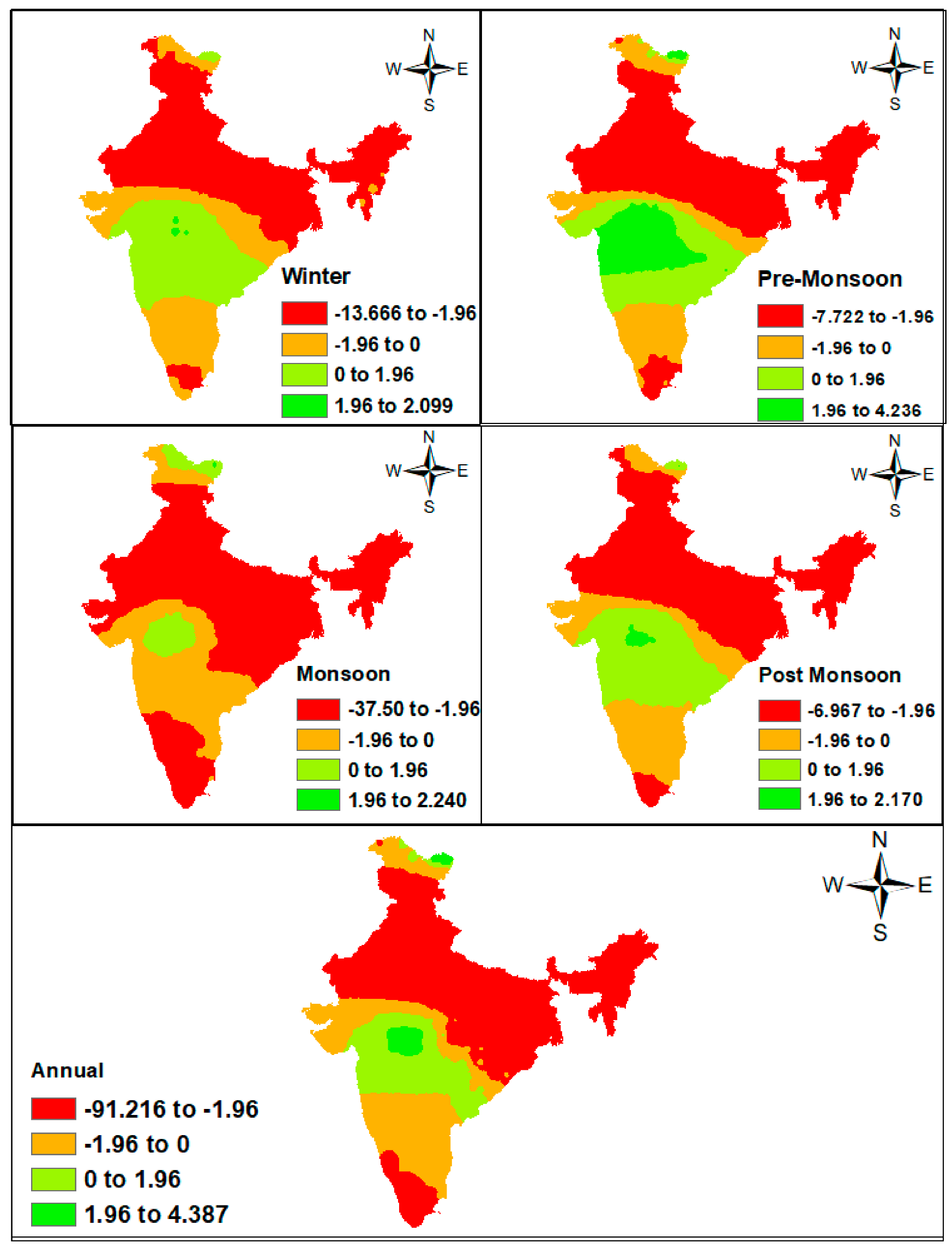
Mann–Kendall and modified Mann–Kendall: In this study, the Z statistics of the winter terrestrial water storage data obtained from the Mann–Kendall test are classified into four parts at a significance level of 95%. These are Z > 1.96 as a significant positive trend, Z in-between 0 and 1.96 as a positive trend, Z in-between 0 and −1.96 as a negative trend, and Z > −1.96 as a significant negative trend. According to this, the results are shown in Figure 6. The data range from −5.4578 (longitude of 77.5, latitude of 30.5) (longitude of 78.5, latitude of 30.5) to 2.0991 (longitude of 76.5, latitude of 21.5) (longitude of 76.5, latitude of 22.5). The same is shown for the modified Mann–Kendall test is shown in Figure 6, and the variation is shown in Figure 7. The data range from −13.6650 (longitude of 78.5, latitude of 33.5) to 2.0991 (longitude of 76.5, latitude of 21.5) (longitude of 76.5, latitude of 22.5). In addition, in this study, according to a significance level of 95%, the p-value is classified into two parts in both the MK and MMK tests. These are H0: there is no trend in the series (p > 0.05), and Ha: there is a trend in the series (p < 0.05), resulting in 49% where p > 0.05 and 51% where p < 0.05. We also find here that the magnitude of the TWS data by Sen’s slope represents that 78% (222 grid points) is negative and 22% (63 grid points) is positive, shown in Figure 8. For the past 19 years, the average slope of the winter terrestrial water storage data from both the MK and MMK tests is −0.0066 m (−6.6 mm). The monotonic trend is represented by Kendall’s tau. According to this, 73% (208 grid points) was negative, whereas 27% (77 grid points) was positive.
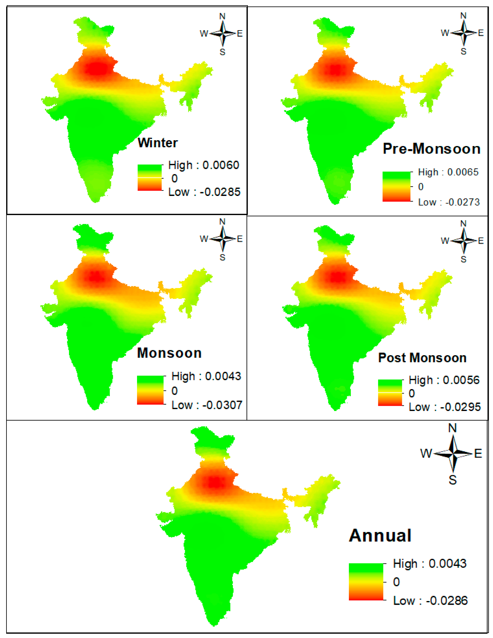
Linear regression analysis: The average slope of winter terrestrial water storage data for over 19 years is found to be −0.0060 m (−6.025 mm) using a linear regression analysis. Winter data revealed 74% negative trends and 26% positive trends, shown in Figure 9, with values ranging from −0.0285 m (longitude of 77.5, latitude of 29.5) to 0.006 m (longitude of 77.5, latitude of 29.5) (longitude of 76.5, latitude of 21.5).

3.2.2. Pre-Monsoon Season

Autocorrelation: Similar to the above three seasons, autocorrelation test results show 45% (129 grid points) where p > 0.05 and 55% (156 grid points) where p < 0.05, with values ranging from 0.00041 to 0.9964.
Mann–Kendall and modified Mann–Kendall: Similar to the above three seasons, the Z statistics of the Mann–Kendall and modified Mann–Kendall test results are shown in Figure 6 and the variation is shown in Figure 7. For the Mann–Kendall test, the data vary from −5.1778 (longitude of 77.5, latitude of 29.5) (longitude of 78.5, latitude of 29.5) (longitude of 78.5, latitude of 30.5) to 2.2390 (longitude of 79.5, latitude of 35.5), and from the modified Mann–Kendall test the data vary from −6.96616 (longitude of 78.5, latitude of 33.5) to 2.1691 (longitude of 75.5, latitude of 21.5) (longitude of 76.5, latitude of 21.5). Similarly, the p-value at a 95% significance level shows 44% where p > 0.05 and 56% where p < 0.05. In addition, we find that the magnitude of TWS data by Sen’s slope represents 83% negative (237 grid points) and 17% positive (48 grid points), shown in Figure 8. For the past 19 years, the average slope of post-monsoon terrestrial water storage data from both the MK and MMK tests is −0.008054 m (−8.054 mm). According to Kendall’s tau, 75% (215 grid points) is negative, whereas 25% (70 grid points) is positive.
Linear regression analysis: The average slope of post-monsoon terrestrial water storage data is −0.006790 m (−6.79 mm) for 19 years (2002–2020). The post-monsoon data revealed 74% negative trends and 26% positive trends, with values ranging from −0.02946 m (longitude of 77.5, latitude of 28.5) to 0.005583 m (longitude of 77.5, latitude of 28.5). A longitude of 76.5 and a latitude of 21.5 are shown in Figure 9.

3.2.3. Monsoon Season

Autocorrelation: Similar to the above two seasons, autocorrelation test results show 29% (83 grid points) where p > 0.05 and 71% (202 grid points) where p < 0.05, with values ranging from 0.0001 to 0.9343.
Mann–Kendall and modified Mann–Kendall: Similar to the above two seasons, the Z statistics of the Mann–Kendall and modified Mann–Kendall test results are shown in Figure 6, and the variation is shown in Figure 7. For the Mann–Kendall test, the data vary from −5.1778 (longitude of 77.5, latitude of 29.5) (longitude of 78.5, latitude of 29.5) (longitude of 78.5, latitude of 30.5) to 2.2390 (longitude of 79.5, latitude of 35.5), and from the modified Mann–Kendall test the data vary from −37.4913 (longitude of 88.5, latitude of 25.5) to 2.2390 (longitude of 79.5, latitude of 35.5). Similarly, the p-value at a 95% significance level shows 33% where p > 0.05 and 67% where p < 0.05. In addition, we find that the magnitude of TWS data by Sen’s slope represents 95% negative (271 grid points) and 5% positive (14 grid points), shown in Figure 8. For the past 19 years, the average slope of monsoon terrestrial water storage data from both the MK and MMK tests is −0.009823 m (−9.823 mm). According to Kendall’s tau, 93% (265 grid points) is negative, whereas 7% (20 grid points) is positive.
Linear regression analysis: According to the linear regression analysis, the average slope is found to be −0.009435 m (−9.435 mm). In addition, we find that, in the linear regression analysis, 95% of monsoon data where the slope is negative. Only 5% of the data represents a positive slope, and the values range from −0.03079 m (longitude of 77.5, latitude of 28.5) to 0.004280 m (longitude of 77.5, latitude of 28.5). A longitude of 79.5 and a latitude of 35.5 are shown in Figure 9.

3.2.4. Post-Monsoon Season

Autocorrelation: Similar to the above three seasons, autocorrelation test results show 45% (129 grid points) where p > 0.05 and 55% (156 grid points) where p < 0.05, with values ranging from 0.00041 to 0.9964.
Mann–Kendall and modified Mann–Kendall: Similar to the above three seasons, the Z statistics of the Mann–Kendall and modified Mann–Kendall test results are shown in Figure 6, and the variation is shown in Figure 7. For the Mann–Kendall test, the data vary from −5.1778 (longitude of 77.5, latitude of 29.5) (longitude of 78.5, latitude of 29.5) (longitude of 78.5, latitude of 30.5) to 2.2390 (longitude of 79.5, latitude of 35.5), and from the modified Mann–Kendall test the data vary from −6.96616 (longitude of 78.5, latitude of 33.5) to 2.1691 (longitude of 75.5, latitude of 21.5) (longitude of 76.5, latitude of 21.5). Similarly, the p-value at a 95% significance level shows 44% where p > 0.05 and 56% where p < 0.05. In addition, we find that the magnitude of TWS data by Sen’s slope represents 83% negative (237 grid points) and 17% positive (48 grid points), shown in Figure 8. For the past 19 years, the average slope of post-monsoon terrestrial water storage data from both MK and MMK is −0.008054 m (−8.054 mm). According to Kendall’s tau, 75% (215 grid points) is negative, whereas 25% (70 grid points) is positive.
Linear regression analysis: the average slope of post-monsoon terrestrial water storage data is −0.006790 m (−6.79 mm) for 19 years (2002–2020). The post-monsoon data revealed 74% negative trends and 26% positive trends, with values ranging from −0.02946 m (longitude of 77.5, latitude of 28.5) to 0.005583 m (longitude of 77.5, latitude of 28.5). A longitude of 76.5 and latitude of 21.5 are shown in Figure 9.

3.2.5. Annual Mean

Autocorrelation: Furthermore, we analyze 285 grid points of the terrestrial water storage data (period of 2002–2020) annual-wise using autocorrelation. The results show 20% (56 grid points) where p > 0.05 and 80% (229 grid points) where p < 0.05, with values ranging from 0.000067 to 0.96672.
Mann–Kendall and modified Mann–Kendall: Similar to season-wise, the annual data of the Z statistics of both the Mann–Kendall and modified Mann–Kendall test results are shown in Figure 6, and the variation is shown in Figure 7. For the Mann–Kendall test, the data vary from −5.52772 (longitude of 79.5, latitude of 29.5) to 2.6589 (longitude of 79.5, latitude of 35.5), and from the modified Mann–Kendall test the data vary from −91.2172 (longitude of 83.5, latitude of 21.5) to 4.3870 (longitude of 83.5, latitude of 21.5) (longitude of 79.5, latitude of 35.5). Similarly, the p-value at a 95% significance level shows 42% where p > 0.05 and 58% where p < 0.05. In addition, we find that the magnitude of TWS data by Sen’s slope represents 87% negative (249 grid points) and 13% positive (36 grid points), shown in Figure 8. For the past 19 years, the average slope of yearly terrestrial water storage data from both MK and MMK is −0.007524 m (−7.524 mm). According to Kendall’s tau, 80% (227 grid points) is negative, whereas 20% (58 grid points) is positive.
Linear regression analysis: The average slope of yearly terrestrial water storage data for nearly 19 years (2002–2020) is found to be −0.007596 m (−7.596 mm) in the linear regression analysis. Finally, 80% of the yearly mean data indicated negative trends, while 20% showed positive trends, with values ranging from −0.028575 m (longitude of 83.5, latitude of 21.5) to 0.004265 m (longitude of 83.5, latitude of 21.5). A longitude of 79.5 and a latitude of 14.5 are shown in Figure 9.

4. Discussion

The goal of our research is to examine the homogeneity of 285 grid points’ terrestrial water storage anomaly data in India using four homogeneity test methods, including Pettitt’s test, the SNHT, the BRT, and the VNRT, as well as to analyze trends in and magnitude of the data through parametric and nonparametric tests over the period of 2002 to 2020 with a significance level of 95%. Hence, we obtain the most homogeneous or useful data in post-monsoon and the least in monsoon and annual based on useful, doubtful, and suspect, shown in Figure 10.
According to the p-value at a 95% significance level, compared with an alpha of 0.05 [23] for the above four tests, the majority of p-values < 0.05 are found in the northern part (Rajasthan, Delhi, Punjab, Himachal Pradesh, and Jammu and Kashmir) and some upper part of the central (Uttar Pradesh and Uttarakhand), eastern (Bihar, Jharkhand, West Bengal, and Sikkim), and northeastern (Meghalaya, Assam, Arunachal Pradesh, and Nagaland) parts. Similarly, p-values > 0.05 are found in Odisha, Chhattisgarh, and the lower half of Madhya Pradesh. According to the von Neumann ratio test, all seasonal and annual data of the von Neumann ratio (N) < 2, indicating the presence of a change point, which is shown in Figure 3. In addition, we use Pettitt’s test to calculate the breakpoint year. The majority of the breakpoints are present in 2014 for winter, 2012 pre-monsoon, 2011 for monsoon and post-monsoon, and 2008 as well as 2011 for annual; the overall breakpoint is shown in Figure 4.
In our study, the autocorrelation test results clearly show that the autocorrelation p-value, compared to p > 0.05, is less in annual data (20%) and highest in pre-monsoon (54%). Similarly, for p < 0.05 we obtain the lowest results in pre-monsoon (46%) and the highest results in annual (80%). According to this, Jammu and Kashmir, Ladakh, Maharashtra, Manipur, and Mizoram are p > 0.05.
In Figure 7, we compare both the MK and MMK tests season-wise; according to this, in winter, pre-monsoon, and post-monsoon a positive and significant positive trend is found in Maharashtra, Telangana, the upper part of Andhra Pradesh, Odisha, Chhattisgarh, the lower part of Madhya Pradesh, and Gujarat, resulting in a chance of floods. Similarly, the most significant negative trend is found in the northern part (Rajasthan, Delhi, Punjab, Himachal Pradesh, and Jammu and Kashmir), central part (Uttar Pradesh, Uttarakhand, and the upper part of Madhya Pradesh), eastern part (Bihar, Jharkhand, West Bengal, and Sikkim), northeastern part (Meghalaya, Assam, Arunachal Pradesh, Nagaland, Manipur, and Mizoram), and lower part of Tamil Nadu and Kerala, resulting in a chance of droughts.
For monsoons, a positive trend is only found in the southwest part of Madhya Pradesh, the north part of Maharashtra, and the upper part of Ladakh; the rest show negative and significantly negative trends.
In the annual mean, positive and significantly positive trends are found in Maharashtra, the southwest part of Madhya Pradesh, the upper part of Telangana and Andhra Pradesh, the lower part of Chhattisgarh, and the topmost part of Ladakh and the rest show negative and significantly negative trends.
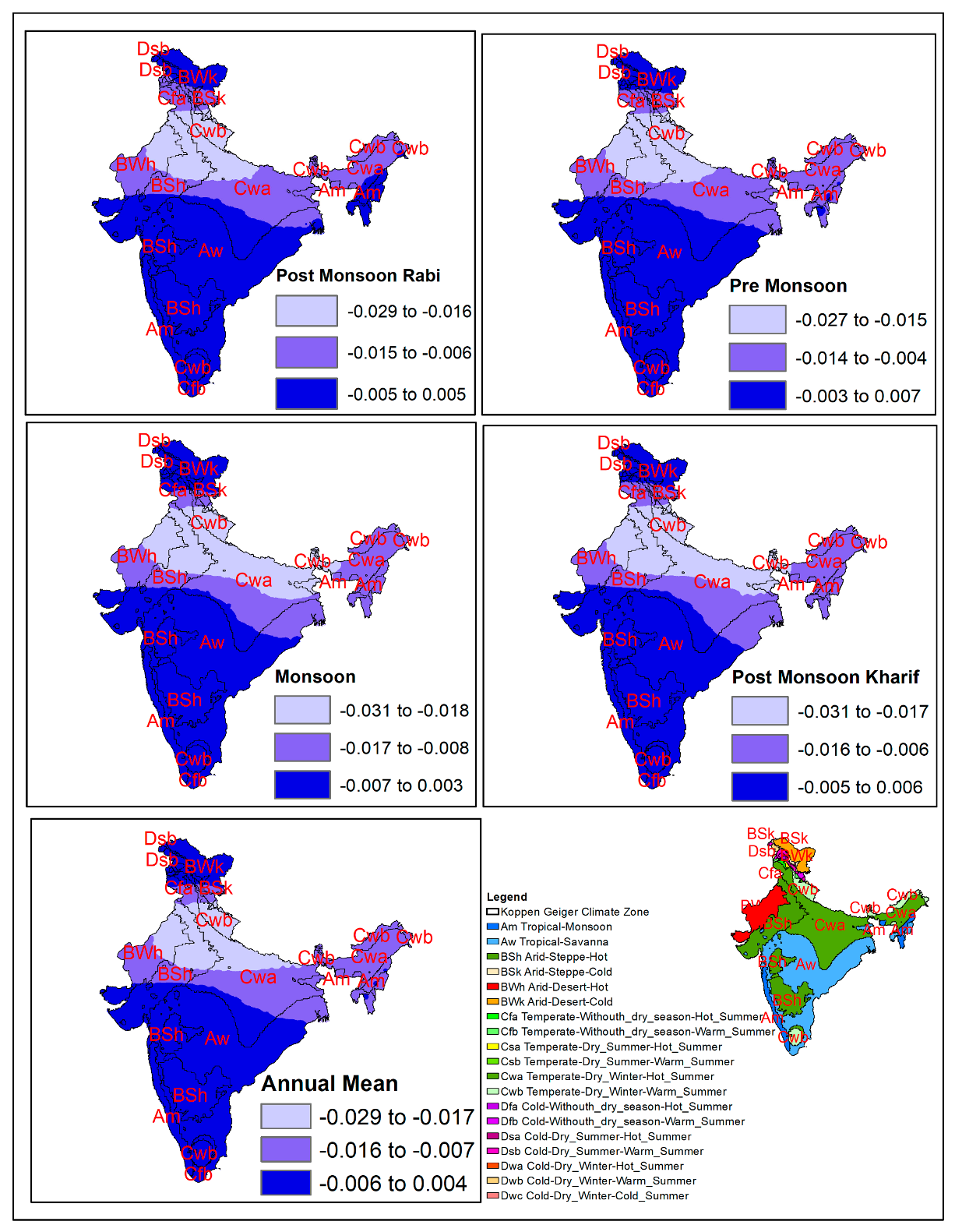
According to Sen’s slope, pre-monsoon has the highest positive magnitude (30%), while monsoons have the highest negative magnitude (about 95%). In the annual average, 13% of the variables have a positive magnitude and 87% have a negative value, shown in Figure 8. TWS changes are declining trends in the MK and MMK tests, as well as the linear regression analysis. The following graph depicts the average slope (Figure 11).
According to Sen’s slope, the most declining magnitude is found in Delhi, Panjab, Uttrakhand, the northern part of Rajasthan, and Uttar Pradesh. According to the simple linear regression analysis, the majority of the declining slope is observed in the same regions outlined above. A modified Mann–Kendall trend test, which is robust in the presence of autocorrelation, is suggested based on these theoretical findings and an empirical approximation; its empirical significance level and power are examined. The updated test was found to be more accurate than the original Mann–Kendall trend test in terms of its empirical significance level, with no loss of power [43].
We further analyze the future trends in TWSA, both seasonally and annually, in different climatic zones, as per Koppen–Geiger described by Peel in 2007 [44], using the modified Mann–Kendall Sen’s slope estimator (cm/year) with zonal statistics and the vector boundaries of climatic zones on a GIS platform. It is important to note that tropical savanna regions show a positive trend in the pre-monsoon season (0.056 cm/year). This also shows the shifting pattern of precipitation from monsoon to pre-monsoon, as it acts as a key hydrological component. Most of the regions of the Indian climate zones show declining future trends in TWSAs, which is a serious challenge for food security and the sustainable development of natural resources. The descriptive statistics of all of the climatic zones are shown in Table 1.

5. Methods

5.1. Homogeneity Test

To investigate homogeneity in terrestrial water storage data, we classify the time series into three categories: homogeneous or useful, doubtful, and inhomogeneous or suspect, based on the null hypotheses and alternative hypotheses (compared with an alpha of 0.05) of four tests: Pettit’s test, the SNHT, the BRT, and the VNRT. The following subsections provide a full overview of the four tests mentioned above [24,45].

5.1.1. Pettitt’s Test (PT)

This test is commonly used to discover change points in metrological time series [19,46]. Pettit’s test is defined as follows:
K T = M a x U t , T 1 i < T
Here ,   U t , T = i = 1 t j = t + 1 T sgn ( x i x j )
The test statistic, Ut,T is calculated from all of the random variables from 1 to n; where the magnitude of the test statistic, |Ut,T|, is highest, the bulk of distinct change points occurs.
It is possible to determine a change point downward or upward depending on large or small values of Ut, i.e., points of inhomogeneity.
The null hypothesis should be rejected and the alternative hypothesis accepted if the p-value is less than the significance level, α. Continuity correction has been made in this case.

5.1.2. Buishand Range Test (BRT)

In this test, the breakpoint primarily occurs at the midpoint of the data series. The test values in the BRT are independent and regularly distributed (null hypothesis). A jump-like movement in the mean is a part of an alternative theory [47]. The adjusted partial sums (cumulative deviations from the mean, x ¯ ) are determined in the BRT using the formula outlined below [23]:
S k = i = 1 k ( x i x ¯ )
where x ¯ is the mean of the series and x i is the time series, where i = t year from 1 to k. Sk may fluctuate around zero inhomogeneous series. When Sk reaches near the year k = K for the maximum and minimum values, that means the breakpoint presents in year K. By plotting S k σ n in a graph over time the evaluation of Sk is represented, where n is the number of observations and σ is the standard deviation. Using the Buishand R statistic, the significance can be calculated in the following equation:
R = m a x S k m i n S k σ
If the value R n > c , the break is significant when c is the critical value.

5.1.3. The Standard Normal Homogeneity Test (SNHT)

For checking homogeneity, this method is the most popular. For hypothesis analyses, SNHT is more sensitive to the breaks around the beginning and end of the time series [20,48]. If we do not reveal whether the data are useful or not, a set of tests is run to obtain good-quality data that can be adopted as a reference.
Alexanderson developed the method of the SNHT in their study. The statistic T(k) is used to compare the mean of the first k years data with the last nk year’s data [20]:
T k = k z 1 2 + n k z 2 2         k = 1 , , n
Here, z 1 ¯ = 1 k i = 1 k ( Y i Y ¯ S ) and z 2 ¯ = i n k i = k + 1 n ( Y i Y ¯ S ) .
As with Pettitt’s test and the Buishand test, it is also the case here that when k = K then T(k) reaches its maximum value, hence the test statistic T0 = T k 1 k n . Wijngaard stated in their study that if T0 is over a given level the null hypothesis is rejected, and the sample size is dependent on it [24].

5.1.4. Von Neumann Ratio Test (VNRT)

The VNR (N), developed by Neumann, is the ratio of the mean square consecutive (year-to-year) difference in δ2/variance in σ2. Where Y1, Y2, …, Yn can be a sequence of observation the equation below is then given [22]:
N = δ 2 σ 2 = i = 1 n 1 ( Y i Y i + 1 ) 2 i = 1 n ( Y i Y ¯ ) 2
Here, the value of N with a parent distribution will determine where some trends exist or if the data are independent. According to the von Neumann ratio (N), it can be classified into three parts:
For N = 2, the series is considered homogeneous [49].
For N < 2, the series with change points are present [24].
For N > 2, the mean of the data series fluctuates rapidly [50].
The VNRT provides no info regarding the change point.
After acquiring the results of the above four tests, the terrestrial water storage data are classified into three criteria [23]:
Homogeneous or useful (HG): The dataset in which none or only one of the four tests above rejects the null hypothesis with a 5% significance.
Doubtful (DF): The series that reject two null hypotheses out of four tests at a 5% significance.
Non-homogeneous or suspect (S): When three or all tests reject the null hypothesis at a 5% significance.
Furthermore, the data are taken into account for additional trend detection analyses as well as the effective evaluation of terrestrial water storage levels for the selected study sites.

5.2. Trend Analysis

Here, we examine the terrestrial water storage trends and changes on seasonal and annual scales over India. Trends are detected using the non-parametric Mann–Kendall test and modified Mann–Kendall test [51]. In addition, Sen’s slope is used to calculate trend magnitude [52]. To acquire reliable results, the autocorrelation of the data is evaluated before applying the Mann–Kendall test. In this paper, we also employ parametric simple linear regression to find the gradient of the TWS.

5.2.1. Autocorrelation

Autocorrelation is used to test the terrestrial water storage data to acquire accurate results in trend analyses. We used the autocorrelation function (ACF) in open source software, R, to test lag1 autocorrelation for all of the time series.

Mann–Kendall Trend Test (MK)

Various strategies are available to detect trends in climatic variability. Most researchers have used the Mann–Kendall [53] and modified Mann–Kendall [54,55,56,57,58] tests to detect trends.
The main advantages of the MK test:
A non-parametric test does not necessitate regularly distributed data.
In non-homogeneous time series it is less susceptible to unplanned interruptions. [26].
In the MK test, the statistic (S) is calculated with the following equation:
S = i = 1 n 1 j = i + 1 n sgn x j x i
where n = no. of data point.
xi and xj = yearly values of years’ i and j, where j > 1 and sgn (θ) is represented by the equation below:
sgn   ( θ ) = + 1 θ > 0 0 θ = 0 1 θ < 0
With zero mean, the “S” statistic is distributed normally, and the variance is as follows:
σ 2 = n n 1 2 n + 5 18
Subsequently, “Z” statistics have a standardized normal distribution:
Z = S 1 θ i f   S > 0 0 i f   S = 0 S + 1 θ i f   S < 0

Modified Mann–Kendall Test (MMK)

In the MK test, there is some problem of serial correlation, so the modified Mann–Kendall test is needed to acquire an accurate trend in the data series; therefore, to eliminate this correlation effect, Yue and Wang introduced the MMK [59]:
n n s = 1 + 2 n n 1 n 2 + k = 1 n 1 n k n k 1 n k 2 p k
n = real length, n s = effective no. of the data, and pk = autocorrelation function of ranks of the data; additionally, V(S) is given as follows:
V S = n n 1 2 n + 5 i = 1 m t i ( t i 1 ) ( 2 t i + 5 ) 18
After corrected variance:
V ( S ) = V ( S )   n n s
The standard normal variable, Z, is calculated as follows:
Z M K = S 1 V S W h e n   S > 0 0 W h e n   S = 0 S + 1 V S W h e n   S < 0
According to a significance level of 95%, the p-value is classified into two parts in both the MK and MMK tests: H0: there is no trend in the series (p > 0.05), and Ha: there is a trend in the series (p < 0.05).

Sen’s Slope Estimator

From Sen’s slope method, we measure the rate of change, which is represented by the equation below [60]:
β i = X j X k j k ;   k     j   and   i = 1 ,   2 ,   3 , ,   N
Here, β = the gradient between Xj and Xk. The SS estimator (β) is considered by the intermediate N values of βi:
β = β N + 1 2 ,   I f   N   i s   O d d β N 2 + β N + 2 2 ,   I f   N   i s   E v e n 2
In our study, to identify the magnitude of change in terrestrial water storage we utilized Sen’s slope estimator. This method is also used by researchers, including the authors of [60,61,62].

5.2.2. Linear Regression Analysis

A parametric way to analyze trend variation is a linear regression analysis. To establish a link between dependent and independent variables, the linear regression approach is used. We employ a regression line to discover long-term seasonal and inter-annual trend patterns in terrestrial water storage change. In our research, we employed the regression formula [63], which is represented by the equation below:
Y = mx + c
where, Y = dependent variable, x = independent variable, m = line slope (unit), and c = intercept constant coefficient. Positive and negative slope values in a linear regression analysis suggest growing and declining trends, respectively.

6. Conclusions

In this study, we analyzed variations in seasonal and annual terrestrial water storage data for 285 grid locations from 2002 to 2020. To determine homogeneity and trends, we used the most recent version of RL06 data from the GRACE and GRACE-FO satellite projects.
For this, most of the homogeneous data are found in winter, pre-monsoon, and post-monsoon, approximately above 42% to 47%, and the least are found in monsoons and annual, only 33%. These homogeneous data are found in the grid points located in Odisha, Chhattisgarh, and the lower half of Madhya Pradesh. According to the von Neumann ratio test, all seasonal and annual data indicate the presence of a change point. According to Pettitt’s test, the majority of the breakpoints are present in 2014 for winter, 2012 for pre-monsoon, 2011 for monsoons and post-monsoon, and 2008 as well as 2011 for annual.
Furthermore, we employed the non-parametric MK test, MMK test, Sen’s slope estimator, and the parametric simple linear regression test to discover long-term trends and magnitudes. According to the MK and MMK tests, the most significant negative trends are found in the northern, central, eastern, northeastern, and lower parts of Tamil Nadu and Kerala, both season- and annual-wise, indicating chances of droughts. Similarly, most of the significant positive trends are found in pre-monsoon (Maharashtra, the lower part of Madhya Pradesh, and Gujarat), resulting in chances of floods. We also observed that the Indo–Gangetic region showed the highest declination, meaning that the northern part has more declining trends than the southern part. According to Sen’s slope, the most declining magnitudes are found in Delhi, Panjab, Uttrakhand, the northern part of Rajasthan, and Uttar Pradesh. Similarly, for the parametric simple linear regression analysis, the majority of the declining slopes are observed in the same regions outlined above. Based on our findings, the average declining rate of yearly terrestrial water storage data from the MK and MMK tests, as well as SLR, is −0.0075 m (−0.75 cm/year) from 2002 to 2020. Most of the regions, such as temperate dry winter and dry semi-arid steppe hot regions, show the highest declining trends in all seasons and annually. On the other hand, tropical monsoon, dry arid, temperate not dry, and continental cold dry regions show the minimum declining trends.
In India, TWSA change is a big concern because of excessive water usage, particularly in agriculture, and poor governance. The conclusions of this study could be useful in planning and managing water resources, agriculture, and the long-term growth of the country. In addition, such findings are significant for any future strategic planning. Such issues can be resolved by managing water resources effectively, using an intelligent water delivery system, and using water sustainably.

Author Contributions

Conceptualization, M.S.U.H., N.A., A.K.R., M.A.K., W.A.K. and Z.M.Y.; data curation, W.A.K.; formal analysis, A.K.R., A.A., W.A.K. and M.K.A.M.; investigation, N.A., M.A.K., M.K.A.M. and Z.M.Y.; methodology, M.S.U.H., M.M.S. and M.A.K.; project administration, M.A.K. and Z.M.Y.; resources, M.S.U.H. and N.A.; software, M.M.S., A.A. and W.A.K.; supervision, M.M.S. and Z.M.Y.; validation, M.S.U.H., M.M.S., N.A., A.K.R., A.A., W.A.K., M.K.A.M. and Z.M.Y.; visualization, N.A., A.K.R., M.A.K., A.A., W.A.K., M.K.A.M. and Z.M.Y.; writing—original draft, M.S.U.H., M.M.S., N.A., A.K.R., M.A.K., A.A., W.A.K., M.K.A.M. and Z.M.Y.; writing—review and editing, M.S.U.H., M.M.S., A.K.R., M.A.K., A.A., W.A.K., M.K.A.M. and Z.M.Y. All authors have read and agreed to the published version of the manuscript.

Funding

This research received no external funding.

Institutional Review Board Statement

Not applicable.

Informed Consent Statement

Not applicable.

Data Availability Statement

Open source data available on their website.

Conflicts of Interest

The authors declare no conflict of interest.

References

  1. Meng, F.; Su, F.; Li, Y.; Tong, K. Changes in Terrestrial Water Storage during 2003–2014 and Possible Causes in Tibetan Plateau. J. Geophys. Res. Atmos. 2019, 124, 2909–2931. [Google Scholar] [CrossRef]
  2. Famiglietti, J.S. Remote sensing of terrestrial water storage, soil moisture and surface waters. Geophys. Monogr. Ser. 2004, 150, 197–207. [Google Scholar]
  3. Huang, Y.; Salama, M.S.; Krol, M.S.; Van Der Velde, R.; Hoekstra, A.Y.; Zhou, Y.; Su, Z. Analysis of long-term terrestrial water storage variations in the Yangtze River basin. Hydrol. Earth Syst. Sci. 2013, 17, 1985–2000. [Google Scholar] [CrossRef] [Green Version]
  4. Güntner, A. Improvement of global hydrological models using GRACE data. Surv. Geophys. 2008, 29, 375–397. [Google Scholar] [CrossRef] [Green Version]
  5. Zhang, Y.; He, B.; Guo, L.; Liu, J.; Xie, X. The relative contributions of precipitation, evapotranspiration, and runoff to terrestrial water storage changes across 168 river basins. J. Hydrol. 2019, 579, 124194. [Google Scholar] [CrossRef]
  6. Zhang, Y.; He, B.I.N.; Guo, L.; Liu, D. Differences in response of terrestrial water storage components to precipitation over 168 global river basins. J. Hydrometeorol. 2019, 20, 1981–1999. [Google Scholar] [CrossRef]
  7. Zhu, Y.; Liu, S.; Yi, Y.; Xie, F.; Grünwald, R.; Miao, W.; Wu, K.; Qi, M.; Gao, Y.; Singh, D. Overview of terrestrial water storage changes over the Indus River Basin based on GRACE/GRACE-FO solutions. Sci. Total Environ. 2021, 799, 149366. [Google Scholar] [CrossRef]
  8. Döll, P.; Douville, H.; Güntner, A.; Müller Schmied, H.; Wada, Y. Modelling Freshwater Resources at the Global Scale: Challenges and Prospects. Surv. Geophys. 2016, 37, 195–221. [Google Scholar] [CrossRef] [Green Version]
  9. Li, X.; Cheng, G.; Ge, Y.; Li, H.; Han, F.; Hu, X.; Tian, W.; Tian, Y.; Pan, X.; Nian, Y.; et al. Hydrological Cycle in the Heihe River Basin and Its Implication for Water Resource Management in Endorheic Basins. J. Geophys. Res. Atmos. 2018, 123, 890–914. [Google Scholar] [CrossRef]
  10. Frappart, F.; Ramillien, G. Monitoring groundwater storage changes using the Gravity Recovery and Climate Experiment (GRACE) satellite mission: A review. Remote Sens. 2018, 10, 829. [Google Scholar] [CrossRef] [Green Version]
  11. Hosseini-Moghari, S.M.; Araghinejad, S.; Ebrahimi, K.; Tang, Q.; AghaKouchak, A. Using GRACE satellite observations for separating meteorological variability from anthropogenic impacts on water availability. Sci. Rep. 2020, 10, 15908. [Google Scholar] [CrossRef]
  12. Iqbal, N.; Evans, T.A.; Saeed, S.; Khan, H.A.A. Evaluation of fipronil baits against Microtermes mycophagus (Blattodea: Termitidae). Can. Entomol. 2016, 148, 343–352. [Google Scholar] [CrossRef]
  13. Mays, L.W. Groundwater Resources Sustainability: Past, Present, and Future. Water Resour. Manag. 2013, 27, 4409–4424. [Google Scholar] [CrossRef]
  14. Rodell, M.; Velicogna, I.; Famiglietti, J.S. Satellite-based estimates of groundwater depletion in India. Nature 2009, 460, 999–1002. [Google Scholar] [CrossRef] [Green Version]
  15. Garduño, H.; Romani, S.; Sengupta, B.; Tuinhof, A.; Davis, R. India Groundwater Governance, A Case Study; Water Partnersh. Program; World Bank: Washington, DC, USA, 2011. [Google Scholar]
  16. Sekhri, S. Sustaining groundwater: Role of policy reforms in promoting conservation in India. Shekhar Shah Barry Bosworth Arvind Panagariya 2013, 149, 149–187. [Google Scholar]
  17. Mukherjee, A.; Ramachandran, P. Prediction of GWL with the help of GRACE TWS for unevenly spaced time series data in India: Analysis of comparative performances of SVR, ANN and LRM. J. Hydrol. 2018, 558, 647–658. [Google Scholar] [CrossRef]
  18. Balachandran, A.; Scientist, D. Central Ground Water Board; Ministry of Water Resources (Government of India): Chennai, India, 2009. [Google Scholar]
  19. Pettitt A Non-parametric to the Approach Problem. Appl. Stat. 1979, 28, 126–135. [CrossRef]
  20. Alexandersson, H. A homogeneity test applied to precipitation data. J. Climatol. 1986, 6, 661–675. [Google Scholar] [CrossRef]
  21. Buishand, T.A. Some methods for testing the homogeneity of rainfall records. J. Hydrol. 1982, 58, 11–27. [Google Scholar] [CrossRef]
  22. Von Neumann, J. Distribution of the Ratio of the Mean Square Successive Difference to the Variance. Ann. Math. Stat. 1941, 33, 1187–1192. [Google Scholar] [CrossRef]
  23. Borah, P.; Hazarika, S.; Prakash, A. Assessing the State of Homogeneity, Variability and Trends in the Rainfall Time Series from 1969 to 2017 and Its Significance for Groundwater in North-East India; Springer: Enschede, The Netherlands, 2021; ISBN 0123456789. [Google Scholar]
  24. Wijngaard, J.B.; Klein Tank, A.M.G.; Können, G.P. Homogeneity of 20th century European daily temperature and precipitation series. Int. J. Climatol. 2003, 23, 679–692. [Google Scholar] [CrossRef]
  25. Hänsel, S.; Medeiros, D.M.; Matschullat, J.; Petta, R.A.; de Mendonça Silva, I. Assessing homogeneity and climate variability of temperature and precipitation series in the capitals of North-Eastern Brazil. Front. Earth Sci. 2016, 4, 1–21. [Google Scholar] [CrossRef]
  26. Tabari, H.; Somee, B.S.; Zadeh, M.R. Testing for long-term trends in climatic variables in Iran. Atmos. Res. 2011, 100, 132–140. [Google Scholar] [CrossRef]
  27. Wang, Y.; Xu, Y.; Lei, C.; Li, G.; Han, L.; Song, S.; Yang, L.; Deng, X. Spatio-temporal characteristics of precipitation and dryness/wetness in Yangtze River Delta, eastern China, during 1960–2012. Atmos. Res. 2016, 172–173, 196–205. [Google Scholar] [CrossRef]
  28. Bari, S.H.; Rahman, M.T.U.; Hoque, M.A.; Hussain, M.M. Analysis of seasonal and annual rainfall trends in the northern region of Bangladesh. Atmos. Res. 2016, 176–177, 148–158. [Google Scholar] [CrossRef]
  29. Bisht, D.S.; Chatterjee, C.; Raghuwanshi, N.S.; Sridhar, V. Spatio-temporal trends of rainfall across Indian river basins. Theor. Appl. Climatol. 2018, 132, 419–436. [Google Scholar] [CrossRef]
  30. Singh, R.; Sah, S.; Das, B.; Vishnoi, L.; Pathak, H. Spatio-temporal trends and variability of rainfall in Maharashtra, India: Analysis of 118 years. Theor. Appl. Climatol. 2021, 143, 883–900. [Google Scholar] [CrossRef]
  31. Javari, M. Trend and homogeneity analysis of precipitation in Iran. Climate 2016, 4, 9–13. [Google Scholar] [CrossRef] [Green Version]
  32. Watkins, M.M.; Wiese, D.N.; Yuan, D.N.; Boening, C.; Landerer, F.W. Improved methods for observing Earth’s time variable mass distribution with GRACE using spherical cap mascons. J. Geophys. Res. Solid Earth 2015, 120, 2648–2671. [Google Scholar] [CrossRef]
  33. Hasan, E.; Tarhule, A. Comparison of decadal water storage trends from common GRACE releases (RL05, RL06) using spatial diagnostics and a modified triple collocation approach. J. Hydrol. X 2021, 13, 100108. [Google Scholar] [CrossRef]
  34. Wang, X.-J.; Zhang, J.-Y.; Shahid, S.; Guan, E.-H.; Wu, Y.; Gao, J.; He, R.-M. Adaptation to climate change impacts on water demand. Mitig. Adapt. Strateg. Glob. Chang. 2016, 21, 81–99. [Google Scholar] [CrossRef]
  35. Food and Agriculture Organization. World Food and Agriculture; Food and Agriculture Organization United Nations: Rome, Italy, 2013; Volume 15. [Google Scholar]
  36. Malik, A.; Kumar, A.; Kim, S.; Kashani, M.H.; Karimi, V.; Sharafati, A.; Ghorbani, M.A.; Al-Ansari, N.; Salih, S.Q.; Yaseen, Z.M. Modeling monthly pan evaporation process over the Indian central Himalayas: Application of multiple learning artificial intelligence model. Eng. Appl. Comput. Fluid Mech. 2020, 14, 323–338. [Google Scholar] [CrossRef]
  37. Bhanja, S.N.; Mukherjee, A.; Saha, D.; Velicogna, I.; Famiglietti, J.S. Validation of GRACE based groundwater storage anomaly using in-situ groundwater level measurements in India. J. Hydrol. 2016, 543, 729–738. [Google Scholar] [CrossRef]
  38. Chatterjee, R.; Gupta, B.K.; Mohiddin, S.K.; Singh, P.N.; Shekhar, S.; Purohit, R. Dynamic groundwater resources of National Capital Territory, Delhi: Assessment, development and management options. Environ. Earth Sci. 2009, 59, 669–686. [Google Scholar] [CrossRef]
  39. Hsu, Y.J.; Fu, Y.; Bürgmann, R.; Hsu, S.Y.; Lin, C.C.; Tang, C.H.; Wu, Y.M. Assessing seasonal and interannual water storage variations in Taiwan using geodetic and hydrological data. Earth Planet. Sci. Lett. 2020, 550, 116532. [Google Scholar] [CrossRef]
  40. He, Q.; Chun, K.P.; Sum Fok, H.; Chen, Q.; Dieppois, B.; Massei, N. Water storage redistribution over East China, between 2003 and 2015, driven by intra- and inter-annual climate variability. J. Hydrol. 2020, 583, 124475. [Google Scholar] [CrossRef]
  41. Hasan, M.S.U.; Rai, A.K. Groundwater quality assessment in the Lower Ganga Basin using entropy information theory and GIS. J. Clean. Prod. 2020, 274, 123077. [Google Scholar] [CrossRef]
  42. Landerer, F.W.; Swenson, S.C. Accuracy of scaled GRACE terrestrial water storage estimates. Water Resour. Res. 2012, 48. [Google Scholar] [CrossRef]
  43. Hamed, K.H.; Ramachandra Rao, A. A modified Mann-Kendall trend test for autocorrelated data. J. Hydrol. 1998, 204, 182–196. [Google Scholar] [CrossRef]
  44. Peel, M.C.; Finlayson, B.L.; McMahon, T.A. Updated world map of the Köppen-Geiger climate classification. Hydrol. Earth Syst. Sci. 2007, 11, 1633–1644. [Google Scholar] [CrossRef] [Green Version]
  45. Armanuos, A.M.; Al-Ansari, N.; Yaseen, Z.M. Cross assessment of twenty-one different methods for missing precipitation data estimation. Atmosphere 2020, 11, 389. [Google Scholar] [CrossRef] [Green Version]
  46. Reeves, J.; Chen, J.; Wang, X.L.; Lund, R.; Lu, Q.Q. A review and comparison of changepoint detection techniques for climate data. J. Appl. Meteorol. Climatol. 2007, 46, 900–915. [Google Scholar] [CrossRef]
  47. Verstraeten, G.; Poesen, J.; Demarée, G.; Salles, C. Long-term (105 years) variability in rain erosivity as derived from 10-min rainfall depth data for Ukkel (Brussels, Belgium): Implications for assessing soil erosion rates. J. Geophys. Res. Atmos. 2006, 111, 1–11. [Google Scholar] [CrossRef]
  48. Martínez, M.D.; Serra, C.; Burgueño, A.; Lana, X. Time trends of daily maximum and minimum temperatures in Catalonia (ne Spain) for the period 1975–2004. Int. J. Climatol. 2010, 30, 267–290. [Google Scholar] [CrossRef] [Green Version]
  49. Daba, M.H.; Ayele, G.T.; You, S. Long-term homogeneity and trends of hydroclimatic variables in upper awash river basin, Ethiopia. Adv. Meteorol. 2020, 2020, 8861959. [Google Scholar] [CrossRef]
  50. Bingham, C.; Nelson, L.S.; Bingham, C.; Nelson, L.S. An Approximation for the Distribution of the von Neumann Ratio Linked references are available on JSTOR for this article: An Approximation for the Distribution of the von Neumann Ratio. Technometrics 2016, 23, 285–288. [Google Scholar] [CrossRef]
  51. Salman, S.A.; Shahid, S.; Afan, H.A.; Shiru, M.S.; Al-Ansari, N.; Yaseen, Z.M. Changes in Climatic Water Availability and Crop Water Demand for Iraq Region. Sustainability 2020, 12, 3437. [Google Scholar] [CrossRef] [Green Version]
  52. Salman, S.A.; Shahid, S.; Sharafati, A.; Ahmed Salem, G.S.; Abu Bakar, A.; Farooque, A.A.; Chung, E.-S.; Ahmed, Y.A.; Mikhail, B.; Yaseen, Z.M. Projection of Agricultural Water Stress for Climate Change Scenarios: A Regional Case Study of Iraq. Agriculture 2021, 11, 1288. [Google Scholar] [CrossRef]
  53. Mann, H.B. Non-Parametric Test Against Trend. Econometrica 1945, 13, 245–259. [Google Scholar] [CrossRef]
  54. Daneshvar Vousoughi, F.; Dinpashoh, Y.; Aalami, M.T.; Jhajharia, D. Trend analysis of groundwater using non-parametric methods (case study: Ardabil plain). Stoch. Environ. Res. Risk Assess. 2013, 27, 547–559. [Google Scholar] [CrossRef]
  55. Jhajharia, D.; Dinpashoh, Y.; Kahya, E.; Choudhary, R.R.; Singh, V.P. Trends in temperature over Godavari River basin in Southern Peninsular India. Int. J. Climatol. 2014, 34, 1369–1384. [Google Scholar] [CrossRef]
  56. Dinpashoh, Y.; Mirabbasi, R.; Jhajharia, D.; Abianeh, H.Z.; Mostafaeipour, A. Effect of Short-Term and Long-Term Persistence on Identification of Temporal Trends. J. Hydrol. Eng. 2014, 19, 617–625. [Google Scholar] [CrossRef]
  57. Zamani, R.; Mirabbasi, R.; Abdollahi, S.; Jhajharia, D. Streamflow trend analysis by considering autocorrelation structure, long-term persistence, and Hurst coefficient in a semi-arid region of Iran. Theor. Appl. Climatol. 2017, 129, 33–45. [Google Scholar] [CrossRef]
  58. Praveen, B.; Talukdar, S.; Shahfahad; Mahato, S.; Mondal, J.; Sharma, P.; Islam, A.R.M.T.; Rahman, A. Analyzing trend and forecasting of rainfall changes in India using non-parametrical and machine learning approaches. Sci. Rep. 2020, 10, 10342. [Google Scholar] [CrossRef]
  59. Yue, S.; Wang, C. The Mann-Kendall Test Modified by Effective Sample Size to Detect Trend in Serially Correlated Hydrological Series. Water Resour. Manag. 2004, 18, 201–218. [Google Scholar] [CrossRef]
  60. Sen, P.K. Estimates of the Regression Coefficient Based on Kendall’s Tau. J. Am. Stat. Assoc. 1968, 63, 1379–1389. [Google Scholar] [CrossRef]
  61. Islam, A.T.; Shen, S.; Yang, S.; Hu, Z.; Chu, R. Assessing recent impacts of climate change on design water requirement of Boro rice season in Bangladesh. Theor. Appl. Climatol. 2019, 138, 97–113. [Google Scholar] [CrossRef]
  62. Zinat, M.R.M.; Salam, R.; Badhan, M.A.; Islam, A.R.M.T. Appraising drought hazard during Boro rice growing period in western Bangladesh. Int. J. Biometeorol. 2020, 64, 1687–1697. [Google Scholar] [CrossRef]
  63. Meshram, S.G.; Singh, V.P.; Meshram, C. Long-term trend and variability of precipitation in Chhattisgarh State, India. Theor. Appl. Climatol. 2017, 129, 729–744. [Google Scholar] [CrossRef]
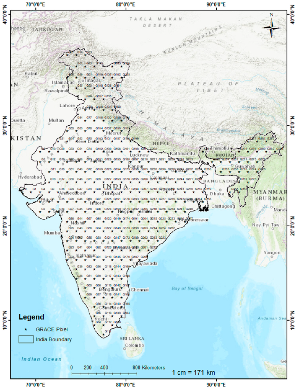
Figure 1. Study area of India showing GRACE pixels from G0 to G284.
Sustainability 15 01572 g001
Figure 2. Flowchart of the methodology adopted in this study.
Sustainability 15 01572 g002
Figure 3. Homogeneity test.
Sustainability 15 01572 g003
Figure 4. The breakpoints detected from seasonal and annual data, with an example.
Sustainability 15 01572 g004
Figure 5. The grid-wise change points of seasonal and annual TWSA data via Pettitt’s test (diamond marks denote the maximum change point in this particular year) (self-made).
Sustainability 15 01572 g005
Figure 6. Z statistics of MK and MMK values.
Sustainability 15 01572 g006
Figure 7. Z statistics (m/year) of seasonal and annual data of TWS by the MMK test.
Sustainability 15 01572 g007
Figure 8. The magnitude of the trends in seasonal and annual TWSA data by the modified Mann–Kendall Sen’s slope estimator (m/year) in different climatic zones.
Sustainability 15 01572 g008
Figure 9. Positive and negative slopes of the TWSA data by a simple linear regression (m/year).
Sustainability 15 01572 g009
Figure 10. Seasonal and annual homogeneity test results.
Sustainability 15 01572 g010
Figure 11. Average slope of 285 grid points, obtained via the MK, MMK, and SLR methods.
Sustainability 15 01572 g011
Table 1. TWSAs’ future Sen’s slope (cm/year) trends based on the modified Mann–Kendall test in different climatic zones in India.
Climate ZoneClimate ZonePMR_MinPMR_MeanPMR_MaxPM_MinPM__MeanPM_MaxM_MinM_MeanM_MaxPMK_MinPMK_MeanPMK_MaxAM_MinAM_MeanAM_Max
BSh Arid-Steppe-HotBSh−2.88−0.660.48−2.7−0.530.69−3.07−0.950.13−3.07−0.710.59−2.91−0.750.37
Dwb Cold-Dry_Winter-Warm_SummerDwb−2.39−0.97−0.4−2.1−0.72−0.1−2.37−0.80−2.49−0.97−0.3−2.29−0.79−0.1
Aw Tropical-SavannaAw−1.3−0.090.5−1.20.0560.67−2.06−0.460.15-1.89−0.190.64−1.55−0.190.42
Cfb Temperate-Withouth_dry_season-Warm_SummerCfb−2.09−1.27−0.3−1.9−1.04−0.2−2−1.06−0.2−2.13−1.22−0.3−1.95−1.07−0.2
Csb Temperate-Dry_Summer-Warm_SummerCsb−2.09−1.27−0.4−1.9−1.1−0.3−1.99−1.16−0.2−2.12−1.25−0.3−1.95−1.14−0.3
Cfa Temperate-Withouth_dry_season-Hot_SummerCfa−1.16−0.76−0.4−1−0.49−0.3−0.96−0.44−0.2−1.08−0.63−0.3−0.94−0.49−0.3
Csa Temperate-Dry_Summer-Hot_SummerCsa−0.98−0.81−0.6−0.8−0.55−0.3−0.74−0.49−0.2−0.9−0.68−0.5−0.78−0.55−0.3
Cwa Temperate-Dry_Winter-Hot_SummerCwa−2.88−1.060.22−2.7−0.950.42−3.07−1.53−0.3−3.07−1.380.28−2.91−1.210.04
Dsb Cold-Dry_Summer-Warm_SummerDsb−2.31−0.78−0.2−2−0.530−2.25−0.50.05−2.39−0.69−0.2−2.18−0.550
BSk Arid-Steppe-ColdBSk−1.38−0.68−0.2−1.3−0.460−1.97−0.450.05−1.84−0.62−0.1−1.6−0.50
Dfa Cold-Withouth_dry_season-Hot_SummerDfa−0.61−0.56−0.5−0.3−0.23−0.2−0.25−0.16−0.1−0.48−0.41−0.4−0.34−0.26−0.2
Cwb Temperate-Dry_Winter-Warm_SummerCwb−2.77−1.39−0.3−2.6−1.27−0.2−2.82−1.51−0.3−2.91−1.55−0.3−2.71−1.4−0.2
Dsa Cold-Dry_Summer-Hot_SummerDsa−0.88−0.64−0.5−0.7−0.38−0.2−0.63−0.31−0.1−0.79−0.52−0.3−0.69−0.4−0.2
BWh Arid-Desert-HotBWh−2.88−1.40.25−2.7−1.260.47−3.02−1.61−0.2−3.04−1.420.34−2.9−1.410.08
BWk Arid-Desert-ColdBWk−1.36−0.320.2−1.3−0.160.28−1.97−0.110.32−1.84−0.260.25−1.59−0.180.31
Am Tropical-MonsoonAm−1.04−0.250.25−1.1−0.20.48−1.8−0.63−0.1−1.67−0.430.34−1.42−0.430.12
Dfb Cold-Withouth_dry_season-Warm_SummerDfb−1.9−1.11−0.4−1.7−0.87−0.2−1.78−0.87−0.1−1.91−1.05−0.3−1.74−0.9−0.2
Dwc Cold-Dry_Winter-Cold_SummerDwc−1.39−1.37−1.3−1.3−1.29−1.3−1.97−1.96−2−1.84−1.84−1.8−1.6−1.59−1.6
Dwa Cold-Dry_Winter-Hot_SummerDwa−0.96−0.9−0.9−0.8−0.7−0.7−0.73−0.66−0.6−0.88−0.82−0.8−0.77−0.72−0.7
Disclaimer/Publisher’s Note: The statements, opinions and data contained in all publications are solely those of the individual author(s) and contributor(s) and not of MDPI and/or the editor(s). MDPI and/or the editor(s) disclaim responsibility for any injury to people or property resulting from any ideas, methods, instructions or products referred to in the content.