Abstract
The urban–rural relationship has been a critical issue in studies on urban and rural geography. Urban–rural integration development (URI), as an integral part of the urban–rural relationship, needs to be understood under an integrated theoretical framework. Based on the conceptual analysis from productivism to post-productivism, this study constructs a multidimensional framework to understand urban–rural integration, restructuring from five layers that integrate population, space, economic, social, and environmental concerns, and the revised dynamic coordination coupling degree (CCD) model is used to measure the level of URI. Many studies have focused on the connection between URI and factor allocation. However, it is yet to be determined how both fiscal decentralization and factor allocation are linked with URI. This study focuses on this unexplored topic, and the impact mechanism among URI, factor allocation, and Chinese-style fiscal decentralization is investigated by adopting spatial econometric models, for achieving the high-quality development of China’s urban–rural relations. Empirical analysis of China’s three major urban agglomerations reveals that there are promising signs in China’s urban–rural integration development, with an orderly and coordinated structure shaping over the period 2003–2017. The rationality of factor allocation depends heavily on the power comparison between the helping hand and the grabbing hand of local governments under Chinese-style fiscal decentralization. Moderate fiscal decentralization, with a perfect market and social security system, leads to the free flow of factors and promotes urban–rural integration. By contrast, excessive fiscal decentralization causes resource misallocation and hinders urban–rural integration development. In light of our empirical evidence, the coordinated development of small- and medium-sized cities and subcities in urban agglomerations is suggested, it is highly necessary to establish a perfect social and employment security system. In addition, a reasonable space planning system for land use needs to be constructed by China’s governments at all levels. Chinese local governments should pay more attention to rural development in their jurisdiction by stimulating their information advantages under Chinese-style fiscal decentralization.
1. Introduction
China has created the world’s largest economic growth miracle [1,2], in which the fiscal decentralization system is considered an important institutional variable [3]. Based on Oates’ definition (1999) [4], fiscal decentralization refers to the fiscal system in which the central government delegates partial tax power to local governments by redividing the power expenditure scope, so that the local governments have the power to decide the budget expenditure structure and scale at their levels. The expansion of fiscal expenditure autonomy can affect the willingness and behavior of the local government to provide public goods and services, as well as the regional economic growth. Stoilova et al. (2018) [5] studied the economic development of six new EU member states—Cyprus, Malta, Slovenia, and the Baltic States of Estonia, Latvia, and Lithuania—and found that fiscal decentralization can effectively improve the budget performance of the member states, and help to promote economic growth. Slavinskaite (2020) [6] evaluated the effect of fiscal decentralization on economic development in particular states of the European Union, and found the effect of fiscal decentralization on the economic development of the EU-13 states to be statistically significant and positive. Wang et al. (2022) [7] found that fiscal decentralization helps local governments to play a greater role in the regional economic system and promotes green economic development in China. Skoromtsova et al. (2022) [8] also proved that fiscal decentralization has a positive influence on the financial development of regions. It can be seen that the scale effect of fiscal decentralization on economic growth has become a general consensus, but there are no consistent conclusions on the impact of fiscal decentralization on the structure of economic growth. Some studies point out that fiscal decentralization can give rise to the information advantages of the local government, reducing the income distribution gap in the process of economic growth. Through the state expenditure report of the National Association of State Budget Officers (NASBO), Swanson et al. (2020) [9] believe that the state government bears more responsibility in funding than the federal government, and that the decentralization of medical assistance will improve poverty. Kumba Digdowiseiso (2022) [10] focused on how the function of institutional quality can explain the relationship between fiscal decentralization and poverty in 53 developing countries from 1990 to 2014, and the findings showed that both revenue and expenditure decentralization were negatively and significantly associated with poverty. Qi et al. (2022) [11] proved that fiscal decentralization is significantly conducive to the industrial green transformation, and the impact of fiscal expenditure decentralization in promoting industrial green transformation is significantly greater than that of fiscal revenue decentralization. On the other hand, some studies have revealed that under the fiscal decentralization system, the assumption of the goal of local government officials to maximize the performance of their responsibilities as “political persons” does not conform to the actual situation. In other words, local government officials, as “rational economic men”, in order to pursue economic growth, may invest more elements of financial resources in the production projects that are conducive to short-term economic growth and increase the local tax revenue, resulting in a “reverse regulation effect” of economic growth. Luo (2017) [12] proved that fiscal decentralization and government competition have a strong “extrusion effect” on public educational investment. Rotulo et al. (2020) [13], using the research cases of Italy, Spain, China, and Cote d’Ivoire, found that the implementation of fiscal decentralization requires the national capital pool to be divided into many local capital pools as a prerequisite contrary to the fiscal federalism. The reorganization of the overall planning system may limit the cross-subsidy effect between high-income and low-income groups and between areas guaranteed by the central government. Therefore, fiscal decentralization reduces medical resources and access to services, resulting in spatial inequality. Cukur (2022) [14] proved that fiscal decentralization leads to a smaller total government and larger central and local governments, which is in line with the prediction of the Leviathan hypothesis in Turkey.
Interestingly, in contrast to the “downward responsible” fiscal federalism in Western countries, the fiscal decentralization in China belongs to the “upward responsibility” [15]. That is, while the central government delegates or transfers financial autonomy or decision-making power to local governments, it retains a highly centralized “personnel administration right”, which directly determines the appointment, removal, and promotion of local government officials. Therefore, the local economic indicators under the fiscal decentralization system are related to the promotion of officials, forming economic decentralization under political centralism [16,17]. Therefore, how does Chinese-style fiscal decentralization affect the quality of economic growth between regions (or between urban and rural areas)? Answering this question is crucial to achieving the goal of high-quality economic development between regions (or between urban and rural areas) in China.
Figure 1 reflects the mutual changes among China’s income distribution, urban and rural income gap, fiscal revenue decentralization (FDR), and fiscal expenditure decentralization (FDE) from 1993 to 2019. It can be seen from Figure 1 that with the increase in fiscal decentralization, the Gini coefficient in China gradually narrows, which indicates that the strengthening of fiscal decentralization can optimize the income distribution gap in China on the whole. However, it is undeniable that after moving past 0.4 in 1994, the Gini coefficient in China has remained between 0.4–0.5, which means that the relative income gap still exists, and from the perspective of changes in urban–rural income gap, this gap is more obvious. In fact, under Chinese-style fiscal decentralization, the major problem in current social and economic development in China is not the problem of “insufficient total output”, but the “structural imbalance”, and the largest “structural imbalance” is reflected in the social and economic fields between urban and rural areas [18,19], which has seriously hindered China’s urban–rural integration development. Therefore, many studies have explored the causes of this phenomenon in Figure 1 from the perspective of factor allocation. Tong et al. [20] pointed out that the urban-biased land use policy makes it difficult to bridge the gap between social and economic development in urban and rural areas. Moreover, under the conditions of incomplete rural collective land rights and obscure property rights in China, it is easy for discrimination and inequality of urban and rural land property rights to occur, resulting in a loss of agricultural land and the damage to farmers’ rights and interests, which is not conducive to balanced urban and rural development. Lu et al. (2017) [21] believe that the lack of an unorganized labor transfer mode is most likely to increase the urban management burden, causing the market crowding effect and competition disruption effect, and ultimately exacerbating the disorder of the urban–rural social and economic development system, which is not conducive to narrowing the gap between urban and rural economic development. Masciandaro et al. (2008) [22] and Wu et al. (2015) [23] believe that under the market economy environment, the profitability of capital means that capital always flows from regions with relatively low returns to regions with relatively high returns, which, therefore, causes changes in resource allocation in different regions and departments, thus resulting in injustice.
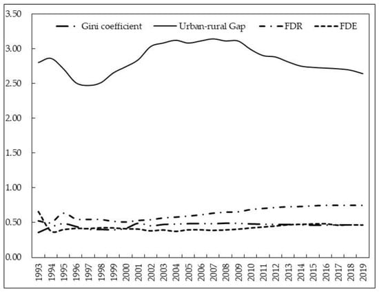
Figure 1.
Changes in fiscal decentralization, Gini coefficient, and urban–rural per capita income gap during 1993–2019.
The “integrated development of urban and rural areas” in China is a holistic and comprehensive concept. It not only depicts the integration of urban and rural monetary categories (such as economy), but also includes the integration of more nonmonetary categories. Unfortunately, the above studies failed to discuss these aspects. Additionally, few scholars pay attention to the interaction mechanism among fiscal decentralization, factor allocation, and the integrated rural–urban development. What kind of impact will the Chinese-style fiscal decentralization have on the integrated development of urban and rural areas? What is the internal logical relationship among fiscal decentralization, factor allocation, and the integrated urban–rural development? This study selects the region with the fastest economic scale development in China as the research object, and deeply explores those puzzles, so as to provide governance experience in urban and rural development for other similar areas or other developing countries. Compared with the existing research, innovations are made in this study in the following aspects: Firstly, the indicators characterizing the social and economic development in urban and rural areas are expanded to the categories of nonmonetary in current China. That is, the multiple dimensions of society, economy, population, space, and ecological environment in the process of the integrated development of urban and rural areas are comprehensively considered, so as to make up for the fact that the existing research only focuses on the urban–rural income gap. Secondly, the linkage effect between fiscal decentralization and factor allocation is fully reflected, and the fiscal decentralization, factor allocation, and the integrated urban–rural development are included in the same framework for theoretical and empirical analysis, thus expanding the theoretical analysis framework of the existing relevant research. Finally, spatial heterogeneity analysis is carried out on the sample areas with different political status, economic development level, and resource endowment characteristics in this paper, so as to provide targeted theoretical and practical reference to the implementation of differentiated urban and rural development policies.
2. Theoretical Framework
2.1. Reconstruction of URI: From Productivism to Post-Productivism
China’s urban–rural relationship has mainly experienced three stages since 1949, as shown in Figure 2. The initial stage was the productivism stage (1949–1978), in which the urban and rural areas were opposite and isolated under the planned economic era. The next was a transition stage between productivism and post-productivism (1978–2003), in which the planned economy transformation and the market economy were established initially. Due to the planned market economy system and Chinese-style fiscal decentralization, the urban–rural relationship was changed from being opposite and isolated to being relaxed and coordinated. With a deepening reform of the socialist market economy and Chinese-style fiscal decentralization, the urban–rural relationship eventually entered into the integration stage (2003–present), where the social and economic development of urban and rural areas are endowed with the characteristic of post-productivism [24,25]. Therefore, the concept of urban–rural integration (URI) needs to be reconstructed under the post-productivism stage.
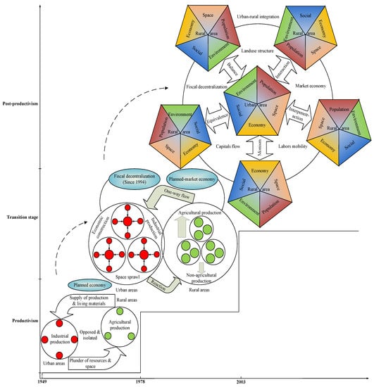
Figure 2.
The evolution of China’s urban–rural relationship.
In particular, the dominant functions of rural areas were agricultural production and rural residents, whereas the urban areas were dominated by modern industries and nonagriculture in the stage of productivism [26]. A large number of production and living materials were transferred from the agricultural sector to the industrial sector, resulting in the sustainable development of rural areas being impeded as resources and space are plundered [27,28]. In the transition stage, the multifunction that combined the agricultural and nonagricultural production of rural areas emerged, while urban areas were still dominated by industrial production and residence. The production factor flows were mainly manifested as one-way flows from rural areas to urban areas. The reaction of urban areas, such as economic development and space sprawl, would also affect the development of rural areas [29,30]. Agriculture, farmers, and rural areas have experienced historic changes since the age of post-productivism; the agricultural functions are not limited to grain production but combine supply, social security, industry consecration, employment guarantee, and ecology [31]. The stratification of peasants is not only reflected in their various occupations but also in some qualitative changes. Moreover, rural values in the natural landscape and traditional culture have also been rediscovered [32].
Therefore, the content of URI has been continuously enriched from economic growth in productivism to multidimensional coordinated development in post-productivism, resulting in changes to the flow of the labor force and capital element and the change in land use structure [33,34]. According to a previous study by Zhou et al. (2020) [35], the Chinese-style urban–rural integration aims to redefine the dominant function of urban and rural sections in spatial production, meaning to fully tap the potential of rural production, and achieve the multidimensional and two-way integration of urban and rural areas based on the objective differences and their respective comparative advantages between urban and rural areas. However, it should be highlighted that the urban–rural integration under the concept of equivalence is not the “homogenization” of no difference, nor the pursuit of the transformation from “heterogeneous space” to “homogeneous space”, but the emphasis on “different but equal” between urban and rural areas. Thus, the URI In post-productivism is classified into five subtypes: urban–rural population integration (URIpo), urban–rural space integration (URIsp), urban–rural economic integration (URIec), urban–rural social integration (URIso), and urban–rural ecological environment integration (URIee). URIpo means equal opportunities in education and employment, etc., and accelerates the interaction of urban–rural residents. URIsp is defined as the interpenetration of urban–rural space, with reasonable land use and a perfect infrastructure. URIec and URIso indicate that the living standard, quality of life, and health condition of urban and rural residents are monistic and equalized. The essence of URIee is maintaining green production, increasing material utilization efficiency, and helping the urban and rural ecosystems to be balanced [36]. An evaluation system of URI is set up by adopting three-level structural models, including the index layer, criterion layer, and target layer. Table 1 shows the explanation and calculation formula of each index.

Table 1.
Evaluation index system of URI.
2.2. Fiscal Decentralization, Factor Allocation, and URI: “Helping Hand” or “Grabbing Hand”?
As local governments have the dual attributes of “helping hand” and “grabbing hand” in allocating production factor between urban and rural areas [22] (see Figure 3), more discretion in economic affairs and resource allocations are given to local governments for the fiscal decentralization, leading to the expansion of the financial expenditure and strengthening responsibility. Furthermore, fiscal decentralization can promote urban–rural integration due to local governments have a clearer understanding of native residents’ preferences than central and provincial governments [4]. Additionally, the senior leaders of the Chinese central government have always paid close attention to the “three rural issues (agriculture, rural areas, and farmers)”and urban–rural balanced development, and some policies on rural revitalization and urban–rural integration are also proposed. Seeking political rewards and promotion opportunities, most of the local government officials also concentrate more on the urban–rural balanced development [37]. For gaining a good political reputation of local governments, more problems of urban–rural unbalanced development will be solved under Chinese-style fiscal decentralization due to the frequent production factors two-way flow [38]. In conclusion, fiscal decentralization could promote urban–rural integration by stimulating the sense of responsibility and exerting the information advantage of local governments.
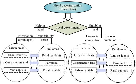
Figure 3.
Impact mechanism of fiscal decentralization, factor allocation, and URI.
It was also found that the horizontal competitions among local governments had been aggravated for the fiscal decentralization reform, resulting in limited production factors that are invested into urban areas for higher marginal returns [39]. Chinese-style fiscal decentralization has created “entrepreneurial local governments”, but it also exacerbates governmental errors due to the characteristics of little decentralization in financial revenue and high centralization in the appointment of local government officials [40]. It would eventually cause the unbalanced and inadequate development of urban and rural areas, such as urban area expansion and high-quality cultivated land being occupied, income gap, and rural male youths’ loss, and even the inequitable public service supplies and deteriorating ecological environment. Hence, the influence of fiscal decentralization on urban–rural integration development in China needs to be specifically tested using practical cases due to its uncertainty.
3. Methodology
3.1. Measuring the Level of URI
The revised dynamic coordination coupling degree (CCD) model [41] is used to measure the level of URI; this model can be used to deal with the panel data. The detailed steps are shown below:
Step 1: Ensure the indexes are distributed in a reasonable range. The upper and lower limit threshold value of each indicator needs to be adjusted by the following two models:
where αi and βi are the maximum and minimum of the raw data; si and li are the revised maximum and minimum values, respectively; xi is the original value, and its standard deviation is σi; D is the coefficient of deviation; k is the adjustment coefficient, and the detailed statistical description of the parameters are shown in Table 2.
Table 2.
Descriptive statistics of parameters.
Step 2: Standardize the indicators using the following two models according to their attributes:
where reveals the effectiveness of xi in the subsystem; if the ui is equal to zero, the coordinated degree of the subsystem is the lowest; if the ui is equal to one, the coordinated degree of the subsystem is the highest.
Step 3: Calculate each dimensional and the comprehensive level of URI using the following two models:
where URImi is the mth dimensional urban–rural integration level at year i, including URIpo, URIsp, URIso, URIee, and URIec.
3.2. Model Specification and Measurement Methods
3.2.1. Spatial Autocorrelation Analysis
Moran’s I statistics are always used to measure the spatial autocorrelation of social and economic occurrences, and they are mainly divided into the Global Moran’s I statistic and Local Moran’s I statistic. The GMI reveals the whole spatial relevance connection, while the LMI shows the characteristics of local spatial accumulation [42].
where I is the GMI statistic, and Ii is the LMI statistic; n is the number of space units, xi and xj are the observed values of samples i and j, respectively; is the average value of the whole sample; wij is the spatial adjacency weight matrix, and this matrix is a binary contiguity matrix. If the two regions are bounded by an adjacent boundary or vertex, the weights matrix value is assigned one; otherwise, it is given a value of zero.
3.2.2. Empirical Model and Variables
The First Law of Geography points out that the development between regions has spatial correlation, and the spatial correlation of things close to each other is greater than that of things far away [43]. As the two main systems of regional development, the traditional measurement method can no longer meet the needs of research on the integrated development of urban and rural areas, and the method has been gradually shifted to the spatial measurement model [44]. The spatial measurement models are mainly divided into a spatial lag model and a spatial error model. The spatial lag model (SLM) analyzes whether the interpreted variable y in a region is affected by the interpreted variable in its surrounding areas:
where W refers to the spatial weight matrix (In this study, the adjacency weight matrix (wit) is applied to the benchmark model. The reasons for choosing this weight matrix are as follows: (a) it is a classical spatial weight matrix; (b) this weight matrix follows the First Law of Geography.); ρ is a vector of the spatial autocorrelation coefficient of y, and α is the constant term; β is the regression coefficient; δ is the spatial lag autoregression coefficient, used to measure the spatial spillover effect of interpreted variables in geographical neighborhood; x is the explanatory variable; ε is the random disturbance term, obeying the independent identical distribution.
If the interpreted variables of a region are also affected by a set of local features and some important variables neglected in geospatial correlation, the spatial error model (SEM) is adopted. The formula is as follows:
where ε refers to the spatial autocorrelation error term; λ refers to the autoregression coefficient of the spatial error term, used to measure the influence degree of the error term of the sample observation value on the interpreted variable.
On the basis of the above theoretical analysis, the interpreted variable is URI. The key explanatory variables include fiscal decentralization and factor allocation (including land, labor, and capital). In consideration of the internal impact mechanism of fiscal decentralization on factor allocation, the cross items are also introduced into the empirical model. Additionally, the specific variable definitions and calculations are as follows: (1) Fiscal decentralization (FD) is measured using the ratio of per capita financial expenditure of local governments and total per capita financial expenditure, consisting of local, provincial, and central governments, meaning the financial autonomy degree of local governments [45]. The larger the indicator is, the more discretion local governments have in social and economic affairs. (2) Factor allocation is divided into three aspects, which are labor mobility (LI), land use structure (LS), and capital flows (CF). Labor mobility between urban and rural areas could affect the URI via the agglomeration effect and diffusing effect [46]; we use the proportion of nonagricultural employment in the total population to measure the LI. The land use structure reveals the spatial interaction relationship between farmland protection and construction land expansion in China’s urbanization [47,48]. Thus, the ratio of cultivated land area and the built-up area is used to measure the LS [49]. Following Wu et al.’s method (2015) [23], the ratio of fixed assets investment between urban and rural areas (In actuality, the impact of capitals on URI in China include fiscal expenditure, fixed assets investment, finance capital, and foreign direct investment (FDI). The reasons for selecting fixed assets investment in the study are (a) eliminating the endogenous problems caused by fiscal expenditure; (b) the effect of fixed asset investment on URI is the most obvious among the four categories.) is used to measure the CF.
In order to alleviate the endogenous problems of missing variables and make the empirical model more practical, a series of control variables are added as follows: (1) PGDP (unit: CNY 10 thousand)—following Udeagha et al.’s (2022) method [50], we use the real GDP per capita to reveal regional economic development; (2) FDE (unit: %), referring to the financial development efficiency, which is calculated using the ratio of the balance of loans and deposits at the end of the year in the financial institution; (3) IND (unit: %), which is measured using the ratio of industrial output in GDP; (4) ADV (unit: %), reflecting the degree of industrial structure upgrading, which is measured using the ratio of the output value between the tertiary industry and the second industry; (5) DFT (unit: %), which is measured using the proportion of the amount of import and export trades in GDP, reflecting the trade openness of one region [51].
3.3. Study Area
As a comparatively complete urban commune, an urban agglomeration consists of various types and scales of cities in a specific region, which are the new centers of China’s economic growth, but also one of the regions where government policy intervention and urban–rural contradiction are more prominent. The study selects China’s top three urban agglomerations as the empirical analysis objects, which are Beijing–Tianjin–Hebei urban agglomeration (UA-BTH), Yangtze River Delta urban agglomeration (UA-YRD), and Pearl River Delta urban agglomeration (UA-PRD). With the most rapid urbanization and the strongest competitiveness, these regions have already attracted international attention in the coordinated development of urban and rural areas. According to the Outline of the Plan for Coordinated Development for the Beijing–Tianjin–Hebei Region, Development Planning for the Yangtze River Delta urban agglomeration (2015–2020), and the Outline of the Plan for the Reform and Development of the Pearl River Delta (2008–2020), they mainly include 49 prefecture-level cities, such as Beijing, Tianjin, Shanghai, Nanjing, Hangzhou, Hefei, Guangzhou, Shenzhen, etc.
3.4. Sources of Data
Most of the sample data were obtained from the China Statistical Yearbook (2004–2018), China Urban Statistical Yearbook (2004–2018), China Rural Statistical Yearbook (2004–2018), and the statistical yearbook of each city. A small amount of missing data were filled by using the interpolation method. There was good compatibility between the different sources of data for the same statistical caliber, and the research period from 2003 to 2017 was chosen because 2003 was the starting point of China’s urban–rural integration development and the statistics were updated in 2017. In order to eliminate price factors, all of the economic indicators (CF, PGDP, FDE, etc.) were calculated at 2007 prices.
4. Results Analysis
4.1. Spatial–Temporal Evolution of URI
The trends of URI in China’s three urban agglomerations are illustrated in Figure 4. The average level of URI increases from 0.22 in 2003 to 0.45 in 2017 with a 1.65% annual growth rate. It is shown that the level of URI in UA-PRD is always in the dominant position with an average level of 0.36. The level of URI in UA-YRD is higher than that in UA-BTH but lower than that in UA-PRD. It can also be seen that the annual growth rate of URI in UA-YRD (1.67) is higher than that of UA-PRD (1.66) and UA-BTH (1.62).
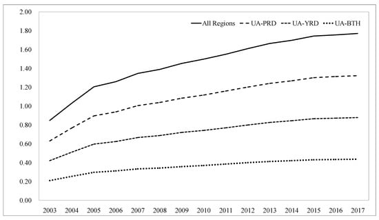
Figure 4.
The trends of URI in China’s three urban agglomerations.
The structures of URI in different dimensions are stable from 2003 to 2017 in Figure 5. The levels of URIec and URIee are always the first and second among all the samples, and the latter one has even become dominant in 2017. There is a slight structural change in each dimensional URI in a specific region. The URIec is always the first. The URIpo and URIsp are the fourth and fifth, respectively, in UA-BTH. The levels of URIee and URIso fluctuate. The URIee is higher than URIso in 2003 and 2017, while that is the opposite in 2010.
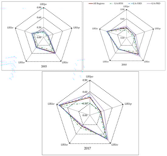
Figure 5.
The structures of URI in different dimensions from 2003 to 2017.
The levels of URIso, URIpo, and URIsp can be seen to decrease in turn during the study period in UA-YRD, while the URIec and URIee are at a correspondingly higher level. The highest levels in 2003 and 2017 are both URIee, and in 2010 it is the URIec. The URIee and URIec are always the first and second in UA-PRD, while the levels of the other dimensions order URIso > URIpo > URIsp in 2003, URIpo > URIso > URIsp in 2010, and URIpo > URIsp > URIso in 2017. Remarkably, the overall structures of different dimensional URI tend to be coordinated and orderly, which corresponds with the goal and demand of making a well-off society in China.
4.2. Spatial Association Analysis of URI
In this study, a positive value of Moran’s I statistic means that high-value areas of URI are adjacent to high-value areas. In contrast, a negative value of Moran’s I statistic indicates that the high-value areas of URI are surrounded by low-value areas. If the Moran’s I statistic is equal to zero, there is a random distribution of URI.
As shown in Figure 6, Moran’s I indexes of UA-BTH and UA-PRD are −0.205 and −0.173, respectively, indicating that the polarization effect of URI in UA-BTH and UA-PRD are extremely obvious. From the Moran scatter plots (Figure 6a), the high values of URI are mainly in the eastern and southern Hebei province, and the low values are in the west and north. The levels of URI in Guangzhou and Shenzhen are very high; the surrounding cities, such as Zhuhai, Huizhou, Zhaoqing, and Jiangmen, show a low level of UA-PRD (Figure 6e). Moran’s I index of UA-YRD is 0.213 (Figure 6c), implying that there is a club convergence phenomena of URI in UA-YRD. Some coastal cities in Zhejiang province, such as Ningbo, Jiaxing, and Zhoushan, show high levels of URI, whereas the unbalanced urban–rural integration development is mainly in the major provincial capitals and municipalities directly under the central government, such as Nanjing, Heifei, and Shanghai. There are local hot spots of URI in northern Zhejiang province and eastern Anhui province, while central-southern and southwestern Anhui province always have low values.
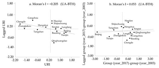
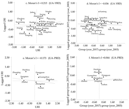
Figure 6.
MI and DMI of URI in the three urban agglomerations.
Differential Moran’s Index (DMI) reveals the reason for the formation of spatial relevance of URI in the three urban agglomerations over time. A positive DMI means that the higher the URI, the faster its growth is; otherwise, it is the reverse. The DMI in UA-BTH (Figure 6b) and UA-PRD (Figure 6f) are, respectively, 0.053 and 0.044, while it is −0.036 in UA-YRD (Figure 6d). Matthew’s effects of hot areas in UA-BTH and UA-PRD cause high-level areas of URI to be surrounded by low-level areas (HL), and vice versa (LH). The catch-up effects of low levels of clustering areas (LL) and diffusion effects of high levels of clustering areas (HH) eventually result in a uniform distribution of URI in UA-YRD.
4.3. Influence Mechanism Analysis
4.3.1. Selection of Spatial Econometric Models
It is inevitable to select a spatial econometric model for estimation due to the spatial relevance of URI, which is verified by Moran’s I statistics. Following Elhorst’s method (2014) [52], a series of Lagrange multiplier tests (LM) are used to select the optimal spatial econometric model. The suitability of fixed effect or random effect is implemented by the Hausman tests. Likelihood ratio tests (LR) are applied to verify the assumptions of individuals nested in both (ind-time) and time nested in both (ind-time).
The results are exhibited in Table 3. The LM spatial lag statistics and robust LM spatial lag statistics are better than LM spatial error statistics and robust LM spatial error statistics, and all of the statistics are significant at the 1% level. Therefore, SLM is selected preferentially. The Hausman tests showed that there are no differences in systematic coefficients between the fixed-effect model and the random-effect model, but the fixed-effect model is preferred to avoid the heteroscedasticity. The original assumptions that individuals nested in both or time nested in both are rejected by the LR tests, so the double-fixed-effects models are adopted.
Table 3.
Estimation results of the LM and LR tests.
4.3.2. Results of the Whole Sample Test
As shown in Table 4, the cross items are ignored in Model (1). It is obvious that the regression coefficient of ln(FD) is significantly positive at the 1% level, meaning that fiscal decentralization promotes urban–rural integration in general. The finding by the “first-generation” of fiscal federalism [53] showed that the average level changed 1% of ln(FD), which leads to a change of 0.061 in URI from the whole sample. The regression coefficient of ln(LI) is 0.316 at the significance level of 10%, indicating that the labor migration between urban and rural areas is a benefit for increasing the level of URI. The misallocation of land and capital between urban and rural areas may have a negative impact on URI, as the regression coefficients of ln(LS) and ln(CF) are −0.005 and −0.001, respectively.
Table 4.
Estimation results of the whole sample and the robust tests.
All of the cross items are introduced into Model (2). The regression coefficients of ln(FD) and ln(LI) are significantly positive, whereas ln(LS) and ln(CF) have a significantly negative impact on URI, which is consistent with Model (1). The ln(LI) has a significantly positive impact on URI, providing further evidence that supports labor mobility, especially the rural labor flows induced by the combination of production and living between urban and rural areas. The excessive cultivated land occupation by urban sprawl had aggravated the rural deterioration [39], as the impact of ln(LS) on URI is significantly negative. According to previous studies, profit-seeking capital may result in a hefty capital gap in rural areas, which eventually aggravates rural poverty [54]. However, the capital inflows into rural areas can ease the resource constraints of agricultural production [55], which inevitably promotes urban–rural integration. Economic growth causes the fixed assets investment inflow into urban areas, which is consistent with the former conclusion. Hence, the coefficient of ln(CF) is significantly negative. The excessive concentration of population under China’s fiscal decentralization and household registration system reform eventually results in the imperfections of social security and the great management pressure of local governments, as the regression coefficient of ln(FD) × ln(LI) is significantly negative, and this finding is in line with China’s reality. The population concentrated mainly in eastern China causes “great urban diseases”, which eventually hinder the development of urban–rural integration in urban agglomerations. Fortunately, the restriction of rural production factors is relieved by the diffusion effect of capital flows for fiscal decentralization, as the ln(FD) × ln(CF) had a significantly positive impact on URI.
In order to ensure the robustness of the results of Model (2), the inverse distance weight matrix and inverse distance square weight matrix (This paper uses the inverse distance weight matrix and inverse distance square weight matrix as the spatial weight matrix, which can better reflect the actual situation of interaction and influence of the flow of factors, etc., for the units that are not contiguous in geographical space.) are introduced into Models (3) and (4), respectively. The significance and sign of most key explanatory variables are consistent with Model (2), indicating that the results are stable and reliable.
4.3.3. Heterogeneity Tests in Different Regions
Heterogeneity test results in different regions are summarized in Table 5. The regression coefficient of ln(FD) is significantly positive in UA-PRD, meaning that the cities are under the jurisdiction of one provincial government (Guangdong province), increasing the level of URI for the free flows of production factors and high-efficiency institutions. In contrast, the ln(FD) has a significantly negative impact on URI due to the different jurisdictions of the cities in UA-YRD. As the cutthroat competition of local governments under fiscal decentralization may increase the distortion of production factor allocation, the urban–rural integration development is restricted. The result supports the above theoretical analysis, namely, that the “helping hand” or “grabbing hand” of local governments depends heavily on the market development and governance efficiency under fiscal decentralization [22]. A moderate fiscal decentralization with perfect market mechanisms and the government’s management system leads to a Pareto allocation of production factors, promoting urban–rural integration. However, excessive discretion in economic and social affairs by extravagant fiscal decentralization increases the distortion of production factor allocation, hindering urban–rural integration development. Beijing, with a high urban primacy index, has attracted a large portion of the labor force, which eventually results in “great urban disease”; this could be the reason that the impact of ln(LI) on URI in UA-BTH is significantly negative. For the UA-YRD and UA-PRD, the regression coefficients of ln(LI) are both significantly positive, indicating that the free flows of the labor force would accelerate urban–rural integration for their balanced development opportunities and similar culture. The ln(LS) has significant negative impacts on URI in the three urban agglomerations. It is the reason that the urban–rural integration development should be hindered by repaid urban area expansion and excessive cultivated land occupation.
Table 5.
Estimation results in the three urban agglomerations.
The insignificance of ln(CF)s in UA-BTH and UA-PRD, indicating the spatial spillover effect of fixed-capital investment, is not exactly stimulated by the huge gap between urban and rural areas. Furthermore, the distorted urban–rural fixed asset investment even has a significant negative effect on URI due to the fierce horizontal competition among local governments in UA-YRD.
The impacts of production factor allocation on urban–rural integration development under Chinese-style fiscal decentralization include regional heterogeneity. The information advantage of local governments can be partly exerted in UA-BTH, but it is not enough to reverse the negative influences of ln(LI) and ln(LS), which is the reason that the regression coefficients of ln(FD) × ln(LI) and ln(FD) × ln(LS) are both insignificant. The positive spillover effect of ln(CF) can be strengthened by fiscal decentralization, and it eventually promotes the urban–rural integration development.
The regression coefficients of ln(FD) × ln(LI) and ln(FD) × ln(LS) in UA-YRD are both significantly positive at the 1% level. It suggests that the “helping hand” of local governments by Chinese-style fiscal decentralization has accelerated labor flows and controlled urban sprawl, resulting in urban–rural integration.
More and more high-quality production resources, such as rural premium quality labors, inflow into the capital city (Guangzhou) and the special economic zone (Shenzhen) in UA-PRD under fiscal decentralization, impeding the development of urban–rural integration. Therefore, the level of URI is reduced marginally by ln(FD) × ln(LI). The impact of ln(FD) × ln(LS) on URI is significantly positive, and this finding is similar to previous research [56,57], namely, that the rise of subcenter cities, such as Zhuhai and Foshan, can relieve the development pressure of central cities because of fiscal decentralization.
The impacts of PGDP on URI are all significantly positive, which is the reason that the regions with a better economic foundation may have better governance in assigning production factors. The regression coefficients of ln(IND) and ADV are almost significantly negative for industrial isomorphism and resource misallocation. The core–periphery distribution structure of financial capital in UA-BTH and UA-PRD restricts urban–rural integration development, whereas a balanced distribution of financial capital in UA-YRD has a positive impact on URI. Thus, the regression coefficients of ln(FDE) in the former two are significantly negative, but are significantly positive in the latter.
5. Conclusions and Policy Implications
Decentralized governance has become a mechanism of national governance, being explored and practiced all over the world, but the promotion of reasonable production factor allocation by the devolution is still confusing, as well as the realization of urban–rural development balances. Previous studies have demonstrated that fiscal decentralization has a two-fold effect [58]. The appropriate decentralization is conducive to the optimal allocation of production elements and promotes urban–rural integration [59]. However, excessive decentralization would lead to production factor misallocation and restrict the urban–rural balanced development [60]. China’s urban–rural relationship has entered the stage of multidimensional integration. Thus, the allocation of resources and factors between urban and rural areas under Chinese-style fiscal decentralization will have a crucial impact on urban–rural integration. This study revisited the dynamic relationship between factor allocation and urban–rural integration development in China over the period 2003–2017 by using the spatial econometric models proposed by Anselin (2013) [61], which can estimate, stimulate, and plot the real spatial association of variables. Using the approaches of the spatial lag model (SLM) and spatial error model (SEM) allows us to identify the positive and negative relationships between ln(FD), ln(LI), ln(LS), ln(CF), ln(FD)×ln(LI), ln(FD) × ln(LS), and ln(FD) × ln(CF) in China; thereby, this study also reconstructs the concept of China’s urban–rural integration that embraces five dimensions of population, space, economic, social, and environmental concerns. In addition, it measures the level of urban–rural integration by using the revised dynamic coordination coupling degree (CCD) model [41], which can overcome the limitations of the traditional coordination coupling degree model. For the robustness check, we used the inverse distance weight matrix and inverse distance square weight matrix to ensure the results are consistent and reliable.
Overall, the results of this study show the following: (1) During the study period (2003–2017), the level of URI of the three major urban agglomerations in China was constantly improving, and the structure of URI also tended to be balanced and stable. From the perspective of spatial heterogeneity, the Pearl River Delta has the highest level of URI, while the Yangtze River Delta has the fastest rate of improvement. However, the development of urban–rural integration in different dimensions also has regional heterogeneity. (2) The spatial correlation analysis shows that the level of URI in China has spatial correlation. More specifically, in the Pearl River Delta and Beijing–Tianjin–Hebei, there is a significant negative spatial correlation, showing a significant polarization effect, while in the Yangtze River Delta, there is a significant positive spatial correlation, with a significant diffusion effect. (3) Chinese-style fiscal decentralization can promote the integration of urban and rural development, and the flow of labor between cities and villages can positively promote the integration of urban and rural areas, but the mismatch of land and capital elements has hindered the integration of urban and rural development to a certain extent. It is worth noting that Chinese central government has paid close attention to the policy orientation of the development of “agriculture, rural areas, and farmers” over the years, which has led to the gradual transition of land and capital elements to a balanced allocation between urban and rural areas under Chinese-style fiscal decentralization. Of course, the specific impact of each explanatory variable on the URI also has spatial heterogeneity.
In light of our empirical evidence, the following policy considerations are suggested: (1) It is necessary to promote the coordinated development of small- and medium-sized cities and subcities in urban agglomerations. A perfect social and employment security system is also needed. Moreover, there is an urgent need to inspire the multifunction of the rural areas and cultivate new farmers. (2) In order to improve the efficiency of construction land and protect rural cultivated land resources, a reasonable space planning system for land use needs to be constructed by China’s governments at all levels. (3) Lastly, equilibrium distribution policies of capital investment among cities could stimulate the diffusion effect of capital from urban to rural areas; thus, local governments should pay more attention to rural development in their jurisdiction.
Although the present work has brought about important empirical findings and significant policy considerations in the case of China, one of the major limitations of this work is that the data only reach up to 2017. Therefore, further studies should explore the changes in recent years, and provide more understanding for a wider research area in China, such as Guangdong Hong Kong Macao Greater Bay Area, Chengdu Chongqing Urban Agglomeration, Central Plains Urban Agglomeration, Guanzhong Plain Urban Agglomeration, etc.
Author Contributions
J.Z. and F.Y. conceived and designed the study; J.Z. completed the paper in English and revised it critically for important intellectual content; F.Y. provided good research advice and revised the manuscript. All authors have read and agreed to the published version of the manuscript.
Funding
This research was supported by the Youth Fund of Western and Frontier Regions for Humanities and Social Sciences of the Ministry of Education of China (Grant No. 22XJC630012), Horizontal Scientific Research Project of Wanzhou Planning and Design Academy of Chongqing of China (Grant No. 2208124).
Data Availability Statement
The data used in this study can be obtained by contacting the corresponding author.
Acknowledgments
We would like to thank the editor and the anonymous reviewers for their helpful suggestions and comments.
Conflicts of Interest
The authors declare no conflict of interest.
References
- Banerjee, A.; Duflo, E.; Qian, N. On the Road: Access to transportation infrastructure and economic growth in China. J. Dev. Econ. 2020, 145, 102442. [Google Scholar] [CrossRef]
- Zhou, X.; Cai, Z.; Tan, K.; Zhang, L.; Song, M. Technological innovation and structural change for economic development in China as an emerging market. Technol. Forecast. Soc. Chang. 2021, 167, 120671. [Google Scholar] [CrossRef]
- Jin, Y.; Rider, M. Does fiscal decentralization promote economic growth? An empirical approach to the study of China and India. J. Public Budg. Account. Financ. Manag. 2022, 34, 146–167. [Google Scholar] [CrossRef]
- Oates, W. Fiscal Federalism; Harcourt Brace Jovanovich: New York, NY, USA, 1972. [Google Scholar]
- Stoilova, D.; Patonov, N. Fiscal decentralization: Is it a good choice for the small new member states of the EU? Sci. Ann. Alexandru Ioan Cuza Univ. Iasi Econ. Sci. Sect. 2012, 59, 125–137. [Google Scholar] [CrossRef]
- Slavinskaite, N. Review of fiscal decentralization in European countries. Int. J. Contemp. Econ. Adm. Sci. 2020, 10, 345–355. [Google Scholar]
- Wang, B.; Liu, F.; Yang, S. Green economic development under the fiscal decentralization system: Evidence from China. Front. Environ. Sci. 2022, 10, 955121. [Google Scholar] [CrossRef]
- Skoromtsova, T.; Chaika, V.; Onishcyik, A.; Holovii, L.; Pankova, L. Fiscal decentralization in the context of Ukraine’s European Integration. J. Int. Commer. Econ. Policy 2022, 13, 2250013. [Google Scholar] [CrossRef]
- Swanson, J.; Ki, N. Has the fiscal decentralization of social welfare programs helped effectively reduce poverty across U.S. States? Soc. Sci. J. 2020. [Google Scholar] [CrossRef]
- Digdowiseiso, K. Are fiscal decentralization and institutional quality poverty abating? Empirical evidence from developing countries. Cogent Econ. Financ. 2022, 10, 2095769. [Google Scholar] [CrossRef]
- Qi, Y.; Zou, X.; Xu, M. Impact of Chinese fiscal decentralization on industrial green transformation: From the perspective of environmental fiscal policy. Front. Environ. Sci. 2022, 10, 1006274. [Google Scholar] [CrossRef]
- Luo, G. Fiscal decentralization, local government competition and investment in public education: An empirical study based on spatial panel model. J. Dalian Univ. Technol. 2017, 38, 131–135. (In Chinese) [Google Scholar]
- Rotulo, A.; Epstein, M.; Kondilis, E. Fiscal federalism vs. fiscal decentralization in healthcare: A conceptual framework. Hippokratia 2020, 24, 107–113. [Google Scholar]
- Cukur, A. Fiscal Decentralization and government size in Turkey: 2009–2020. Maliye Derg. 2022, 182, 108–129. [Google Scholar]
- Ouyang, A.Y.; Li, R. Fiscal decentralization and the default risk of Chinese local government debts. Contemp. Econ. Policy 2021, 39, 641–667. [Google Scholar] [CrossRef]
- Niu, M. Fiscal decentralization in China revisited. Aust. J. Public Adm. 2013, 72, 251–263. [Google Scholar]
- Xu, H.; Li, X. Effect mechanism of Chinese-style decentralization on regional carbon emissions and policy improvement: Evidence from China’s 12 urban agglomerations. Environ. Dev. Sustain. 2022, 25, 474–505. [Google Scholar] [CrossRef]
- Wang, Y.; Huang, Y.; Sarfraz, M. Signifying the relationship between education input, social security expenditure, and urban-rural income gap in the circular economy. Front. Environ. Sci. 2013, 10, 989159. [Google Scholar] [CrossRef]
- Yin, X.; Su, C. Have housing prices contributed to regional imbalances in urban-rural income gap in China? J. Hous. Built Environ. 2022, 37, 2139–2156. [Google Scholar] [CrossRef]
- Tong, D.; Yuan, Y.; Wang, X. The coupled relationships between land development and land ownership at China’s urban fringe: A structural equation modeling approach. Land Use Policy 2021, 100, 104925. [Google Scholar] [CrossRef]
- Lu, M.; Sun, C.; Zheng, S. Congestion and pollution consequences of driving-to-school trips: A case study in Beijing. Transp. Res. Part D Transp. Environ. 2017, 50, 280–291. [Google Scholar] [CrossRef]
- Masciandaro, D.; Quintyn, M. Helping Hand or Grabbing Hand? Supervisory Architecture, Financial Structure and Market View; International Monetary Fund: Washington, DC, USA, 2008. [Google Scholar]
- Wu, Q.; Shi, Y.; Wan, G. Investment tendency and urban-rural gap: Evidence from provincial panel data. World Econ. Pap. 2015, 1, 34–49. [Google Scholar]
- Long, H.; Liu, Y.; Li, X.; Chen, Y. Building new countryside in China: A geographical perspective. Land Use Policy 2010, 27, 457–470. [Google Scholar] [CrossRef]
- Murdoch, J.; Pratt, A. Rural studies: Modernism, post-modernism and the ‘post-rural’. J. Rural Stud. 1993, 9, 411–427. [Google Scholar] [CrossRef]
- Zhang, J.; Shen, M.; Zhao, C. Rural renaissance: Rural China transformation under productivism and post-productivism. Urban Plan. Int. 2014, 29, 1–7. [Google Scholar]
- Ma, L.; Long, H.; Tu, S.; Zhang, Y.; Zheng, Y. Farmland transition in China and its policy implications. Land Use Policy 2020, 92, 104470. [Google Scholar] [CrossRef]
- Yan, J.; Chen, H.; Xia, F. Toward improved land elements for urban–rural integration: A cell concept of an urban–rural mixed community. Habitat Int. 2018, 77, 110–120. [Google Scholar] [CrossRef]
- Zhang, L.; Ge, D.; Sun, P.; Sun, D. The transition mechanism and revitalization path of rural industrial land from a spatial governance perspective: The case of Shunde district, China. Land 2021, 10, 746. [Google Scholar] [CrossRef]
- Ge, D.; Long, H.; Qiao, W.; Sun, D.; Xiong, C. Effect of rural-urban migration on rural production transformation in China’s traditional farming area: A case of Yucheng City. J. Rural Stud. 2020, 76, 85–95. [Google Scholar] [CrossRef]
- Åsa, A.; Patrick, B.; Svante, K.; Linda, L. Beyond post-productivism: From rural policy discourse to rural diversity. Eur. Countrys. 2014, 6, 297–306. [Google Scholar]
- Long, H.; Zou, J.; Pykett, J.; Li, Y. Analysis of rural transformation development in China since the turn of the new millennium. Appl. Geogr. 2011, 31, 1094–1105. [Google Scholar] [CrossRef]
- He, R. Urban-rural integration and rural revitalization: Theory, mechanism and implementation. Geogr. Res. 2018, 37, 2127–2140. (In Chinese) [Google Scholar]
- Zhang, Y.; Long, H.; Tu, S.; Li, Y.; Ma, L.; Ge, D. Analysis of rural economic restructuring driven by e-commerce based on the space of flows: The case of Xiaying village in central China. J. Rural Stud. 2018, 93, 196–209. [Google Scholar] [CrossRef]
- Zhou, J.; Zou, W.; Qin, F. Review of urban-rural multi-dimensional integration and influencing factors in China: Based on the concept of equivalence. Geogr. Res. 2020, 39, 1836–1851. (In Chinese) [Google Scholar]
- Zhou, J.; Qin, F.; Liu, J.; Zhu, G.; Zou, W. Measurement, spatial-temporal evolution and influencing mechanism of urban-rural integration level in China from a multidimensional perspective. China Popul. Resour. Environ. 2019, 29, 166–176. (In Chinese) [Google Scholar]
- Li, H.; Zhou, L. Political turnover and economic performance: The incentive role of personnel control in China. J. Public Econ. 2004, 89, 1743–1762. [Google Scholar] [CrossRef]
- Andreas, K.; Albert, S.; Andreas, S.; Timo, V. Does fiscal decentralization foster regional investment in productive infrastructure? Eur. J. Political Econ. 2013, 31, 15–25. [Google Scholar]
- Weingast, B. Second generation fiscal federalism: The implications of fiscal incentives. J. Urban Econ. 2009, 65, 279–293. [Google Scholar] [CrossRef]
- Feltenstein, A.; Iwata, S. Decentralization and macroeconomic performance in China: Regional autonomy has its costs. J. Dev. Econ. 2005, 76, 481–501. [Google Scholar] [CrossRef]
- Feng, C.; Zhang, J.; Yang, Z. Evaluation of spatial coordination of regional land use for undertaking industrial transfer. China Popul. Resour. Environ. 2015, 25, 144–151. (In Chinese) [Google Scholar]
- Anselin, L. Local indicators of spatial association: LISA. Geogr. Anal. 1995, 27, 93–115. [Google Scholar] [CrossRef]
- Tobler, W. On the first law of geography: A reply. Ann. Assoc. Am. Geogr. 2004, 94, 304–310. [Google Scholar] [CrossRef]
- Zhou, J.; Bi, X.; Zou, W. Driving mechanism of urban-rural integration in Huaihai Economic Zone: Based on the space of flow. J. Nat. Resour. 2020, 35, 1881–1896. [Google Scholar]
- Guo, Q.; Jia, J. Fiscal decentralization, government structure and local government’s expenditure size. Econ. Res. J. 2010, 45, 59–72. (In Chinese) [Google Scholar]
- Pontus, B.; Ding, D.; Per, T. Labour market mobility, knowledge diffusion and innovation. Eur. Econ. Rev. 2020, 123, 103386. [Google Scholar]
- Li, J.; Liu, Y.; Yang, Y.; Jiang, N. County-rural revitalization spatial differences and model optimization in Miyun District of Beijing-Tianjin-Hebei region. J. Rural Stud. 2019, 86, 724–734. [Google Scholar] [CrossRef]
- Ge, D.; Lu, Y. A strategy of the rural governance for territorial spatial planning in China. J. Geogr. Sci. 2021, 31, 1349–1364. [Google Scholar] [CrossRef]
- Huang, Z.; Du, X.; Carlos, S.; Zepeda, C. How does urbanization affect farmland protection? Evidence from China. Resour. Conserv. Recycl. 2019, 145, 139–147. [Google Scholar] [CrossRef]
- Udeagha, M.; Ngepah, N. Does trade openness mitigate the environmental degradation in South Africa? Environ. Sci. Pollut. Res. 2022, 29, 19352–19377. [Google Scholar] [CrossRef]
- Udeagha, M.; Ngepah, N. Disaggregating the environmental effects of renewable and non-renewable energy consumption in South Africa: Fresh evidence from the novel dynamic ARDL simulations approach. Econ. Chang. Restruct. 2022, 55, 1767–1814. [Google Scholar] [CrossRef]
- Elhorst, J. Matlab software for spatial panels. Int. Reg. Sci. Rev. 2014, 37, 389–405. [Google Scholar] [CrossRef]
- Tiebout, C.M. A pure theory of local expenditures. J. Political Econ. 1956, 64, 416–424. [Google Scholar] [CrossRef]
- Wei, Y.; Zhao, M. Urban spill over vs. local urban sprawl: Entangling land-use regulations in the urban growth of China’s megacities. Land Use Policy 2009, 26, 1031–1045. [Google Scholar]
- Scarlett, E.; David, J. Development—There is another way: A rural-urban partnership development paradigm. World Dev. 2001, 29, 1443–1454. [Google Scholar] [CrossRef]
- Pan, H.B.; Yu, M.G. Helping hand, grabbing hand and inter-province mergers. Econ. Res. J. 2011, 9, 108–120. (In Chinese) [Google Scholar]
- Li, Y.; Liu, Y.; Long, H.; Cui, W. Community-based rural residential land consolidation and allocation can help to revitalize hollowed villages in traditional agricultural areas of China: Evidence from Dancheng County, Henan Province. Land Use Policy 2014, 39, 188–198. [Google Scholar] [CrossRef]
- Qiao, M.; Ding, S.; Liu, Y. Fiscal decentralization and government size: The role of democracy. Eur. J. Political Econ. 2019, 59, 316–330. [Google Scholar] [CrossRef]
- Golem, S. Fiscal decentralization and the size of government: A review of the empirical literature. Ann. Clin. Biochem. 2010, 43, 135–145. [Google Scholar]
- Song, Y. Rising Chinese regional income inequality: The role of fiscal decentralization. China Econ. Rev. 2013, 27, 294–309. [Google Scholar] [CrossRef]
- Anselin, L. Spatial Econometrics: Methods and Models; Springer Science & Business Media: Berlin/Heidelberg, Germany, 2013; pp. 69–79. [Google Scholar]
Disclaimer/Publisher’s Note: The statements, opinions and data contained in all publications are solely those of the individual author(s) and contributor(s) and not of MDPI and/or the editor(s). MDPI and/or the editor(s) disclaim responsibility for any injury to people or property resulting from any ideas, methods, instructions or products referred to in the content. |
© 2023 by the authors. Licensee MDPI, Basel, Switzerland. This article is an open access article distributed under the terms and conditions of the Creative Commons Attribution (CC BY) license (https://creativecommons.org/licenses/by/4.0/).