Short-Term Traffic Flow Prediction Based on the Optimization Study of Initial Weights of the Attention Mechanism

Abstract

Traffic-flow prediction plays an important role in the construction of intelligent transportation systems (ITS). So, in order to improve the accuracy of short-term traffic flow prediction, a prediction model (GWO-attention-LSTM) based on the combination of optimized attention mechanism and long short-term memory (LSTM) is proposed. The model is based on LSTM and uses the attention mechanism to assign individual weight to the feature information extracted via LSTM. This can increase the prediction model’s focus on important information. The initial weight parameters of the attention mechanism are also optimized using the grey wolf optimizer (GWO). By simulating the hunting process of grey wolves, the GWO algorithm calculates the hunting position of the grey wolf and maps it to the initial weight parameters of the attention mechanism. In this way, the short-time traffic flow prediction model is constructed. The traffic flow data of the trunk roads in the center of Qingdao (China) are used as the research object. Multiple sets of comparison models are set up for prediction analysis. The results show that the GWO-attention-LSTM model has obvious advantages over other models. The prediction error MAE values of the GWO-attention-LSTM model decreased by 7.32% and 14.35% on average compared with the attention-LSTM model and LSTM model. It is concluded that the GWO-attention-LSTM model has better model performance and can provide effective help for traffic management control and traffic flow theory research.

1. Introduction

The urban transportation system is the basis for supporting the rapid development of the city, which significantly affects the economic development of the city. The traffic problem involves people’s daily travel and affects people’s quality of life at the same time. With the increasing number of motor vehicles and the reduction of urban land, the problem of road congestion has become increasingly serious. How to improve the current situation of traffic congestion has become an important topic affecting economic development and social stability [1]. An intelligent traffic system (ITS) [2] can use high-tech means to accurately analyze and judge urban road problems. Among them, short-term traffic prediction, as one of the hot topics in ITS research, can provide real-time and reliable information to travelers, so as to help alleviate traffic congestion, optimize travel routes, and reduce automobile exhaust emissions.

At present, there are many traffic flow prediction methods, including the mathematical statistical analysis model [3], regression prediction model [4], machine learning prediction model [5,6], and artificial neural network prediction model [7,8]. In recent years, the attention mechanism has been widely used in the research of traffic flow prediction, and has achieved good results [9,10]. Although the methods of traffic flow prediction are diverse and advanced, there are still many problems to be solved:

(1) In the practical application of traffic flow prediction, it is usually difficult to obtain comprehensive data such as weather, spatiotemporal factors, and travel interest points. Therefore, it is necessary to improve the accuracy of traffic flow prediction with a single input factor.

(2) At present, there are a lot of prediction models combining the attention mechanism. However, there is a lack of research on optimizing the initial weight parameters of the attention mechanism.

(3) The traffic flow time series has strong nonlinearity and randomness. In order to pursue better model performance, it is usually necessary to increase the depth of the model. This will increase the calculation cost of the model and make it difficult to converge.

For problem (1), a single input factor can be obtained in most cases. However, the traffic flow time series has strong randomness, so it is necessary to strengthen the prediction model. The attention mechanism is added to the LSTM network. Through the method of weight distribution, the importance of the feature information extracted from each unit is scored to improve the model’s attention towards important information. For problem (2), when we disassemble the operation process of the attention mechanism, we find that the initial weight parameter of the attention mechanism is very important. Therefore, the GWO algorithm is considered to optimize the initial weight parameters of the attention mechanism. The optimal gray wolf hunting position in high-dimensional space is taken as the optimal solution of initial weight parameters. For problem (3), it is very difficult to solve the problem that the model structure is too complex. The GWO optimization algorithm is added to the model proposed in this paper, which can significantly improve the convergence speed of the model. The main contributions of this paper are as follows:

(1) Accuracy of traffic flow prediction with single input factor is improved. Due to the strong data availability of the single factor, this method has wide applicability.

(2) The GWO-attention-LSTM model is established to solve the problem of the strong uncertainty of the weight parameter value. At the same time, it solves the problem that complex models are difficult to train. This makes the performance of the model better and the prediction results more stable.

(3) The research object is the actual road section data of Qingdao. Compared with many existing models, it is proved that the model proposed in this paper has higher accuracy and better stability.

2. Related Research

With the significant increase in data, the research methods of traffic flow prediction are mainly divided into regression analysis prediction and machine learning prediction. For example, He et al. (2000) used a more stable stepwise regression analysis method to construct a prediction model by studying multiple sets of roadway data and achieved good, expected results [11]. Williams et al. (2003) arranged and analyzed traffic flow data in chronological order. They found that the traffic flow was seasonal. Therefore, an autoregressive comprehensive moving average process theoretical prediction model considering seasonal factors had been developed [12]. Clark (2003) used a non-parametric regression-based pattern-matching technique to generate forecasts [13]. The non-parametric regression was multivariate, extended according to the characteristics of the traffic state. A study of actual data from London’s orbital freeways was carried out and the technique proved to be a reliable predictor. The above regression analysis prediction methods have the advantages of simple operation and fast computation time. However, the traffic flow time series usually have strong randomness, and the traditional regression model is difficult to fit a large amount of data into.

Within the context of the big data era, the machine-learning model can effectively process a large amount of input data. Xiong et al. (2020) considered that the traditional prediction methods are at a shallow level for the study of traffic flow characteristics [14]. The spatiotemporal features in the traffic flow time series data were extracted. The random forest (RF) model was used as the output module of the prediction. The superiority of this RF combination model was demonstrated by comparing the prediction results of traditional models. But RF includes two important parameters: the number of decision trees to be built and the maximum depth of a single decision tree. It is difficult to find the best combination of parameters to obtain the best prediction results. Therefore, the RF model parameters need to be optimized. Zou et al. (2021) used the strong optimization-seeking ability of the particle swarm improvement algorithm to calculate the best parameter matching case that can maximize the performance of the support vector machine (SVM), which effectively improved the prediction effect of the model [15]. However, the SVM runs very slowly in order to meet a certain level of accuracy. Therefore, when the randomness of the input sequence is strong and high accuracy is required, the SVM is not easy to be trained. Lin et al. (2022) proposed to combine the SVM with the k-nearest neighbor (KNN) and transformed traffic flow time series into a traffic state vector [16]. The proposed model was used for the traffic flow prediction. The results showed that the prediction error of the model is greatly reduced. However, the structure of the KNN model is simple, and it cannot excavate the deep characteristics of the traffic flow time series.

Machine learning models are highly adaptable and fast to train, but the above models lack the deep feature mining of the traffic flow time series, so it is difficult to capture the hidden patterns in the time series. With the development of artificial neural-network technology, prediction models relying on deep learning algorithms have emerged. Deep learning algorithms are good at deep mining feature information in data and have a stronger nonlinear fitting ability, which is a new research direction [17]. Wang et al. (2020) optimized the parameters of the BP network to find the optimal critical value and weight value of the BP network [18]. Compared with the traditional BP network [19], the improved BP network had better model performance. Hochreiter (1997) proposed the long short-term memory (LSTM) network [20]. LSTM is a variant of the RNN, which is widely used in the field of time series forecasting due to its superior performance. Ma et al. [21] (2015), Cao et al. (2018) [22], and Zhong et al. (2019) [23] all used LSTM to build short-time traffic flow prediction models. The LSTM network has a memory function and can obtain the temporal characteristics of historical information. So, the LSTM network has better prediction results compared to traditional artificial neural network models. Li et al. (2019) added a BP network to the LSTM network to further explore the information features of the data, which significantly improved the model’s ability to mine traffic flow information [24]. However, the structure of the deep learning model is complex. A large number of parameters need to be adjusted. In addition, it is also important to accurately predict the traffic flow with missing data [25]. Chen et al. (2021) proposed a Bayesian temporal factorization (BTF) model, which can predict the traffic flow with missing spatiotemporal data [26]. In this model, the process of tensor decomposition and vector autoregression was transformed into a graphical structure to reduce the uncertainty caused by data loss. The BTF model was proved to be superior to the existing methods through the verification of several real spatiotemporal data sets. Wang et al. (2022) proposed a multi-view bidirectional spatiotemporal graph network (Multi-BiSTGN). The model was used to predict the urban traffic flow with missing data [27]. After filling in the data, the author constructed different spatiotemporal map sequences to describe the traffic state. The bidirectional spatiotemporal map network was fused using the parameter matrix method. The real traffic flow data collected from Wuhan were used as the experimental object. It was proved that the Multi-BiSTGN model had a good effect on traffic flow prediction with missing data. Based on the summary and analysis of typical prediction methods at home and abroad, the research status of traffic flow prediction models is shown in

Table 1. The research status of traffic flow prediction models.

Type	Model	Advantage	Disadvantage
Regression prediction model	Stepwise regression analysis model	Simple principle and easy operation	Need amount of historical data
	Autoregressive moving average model	Wide applicability	Weak predictive ability of strong nonlinearity
	Non-parametric regression model	No subjective model	Long training time
Traditional machine learning model	K-Nearest Neighbor model	Simple structure and strong applicability	Unable to deeply mine the characteristics of time series
	Random Forest	Few parameters and easy training	Parameters need to be optimized, easy to over fit
	Support Vector Machine model	Simple structure, high accuracy	Slow convergence and prone to local optima
Deep learning model	Neural network model	Strong nonlinear prediction ability	Many parameters need to be adjusted
	Long Short-Term Memory model	High accuracy and effective mining of time characteristics	Complex model structure
	Spatiotemporal combination model	Comprehensive and high prediction accuracy	The required data is diverse and difficult to obtain

.

As can be seen from Table 1, the structure of the regression model is simple. But the regression model has insufficient prediction ability for strong nonlinear data. Traditional machine learning is easy to be trained, but the model performance is insufficient. The deep learning model has high accuracy, but the structure of the model is complex, which requires a lot of parameter adjustment. Therefore, the existing prediction models cannot be easily trained with high accuracy.

To overcome the above problems, this paper combines the attention mechanism with the LSTM model. By means of a weight assignment, the importance of feature information extracted from each unit is scored to increase the model’s focus on important information. However, the initial weight parameters of the attention mechanism are all randomly taken. In the process of model iteration, the weight values are adjusted according to the set parameters and input information, so there is uncertainty. Therefore, the GWO algorithm is used to optimize the initial weight parameters of the attention mechanism. The optimal gray wolf hunting position in high-dimensional space is taken as the optimal solution of the initial weight parameters. Thus, the short-time traffic flow prediction model based on the GWO-Attention-LSTM is implemented. To verify the superiority of the proposed model, the prediction results of the GWO-Attention-LSTM model are compared with the attention-LSTM model, LSTM model, RNN model, SVM model, ARIMA model and historical average method (HAM) model, respectively. Several groups of typical urban roads in different locations are selected for prediction analysis.

3. Methodologies

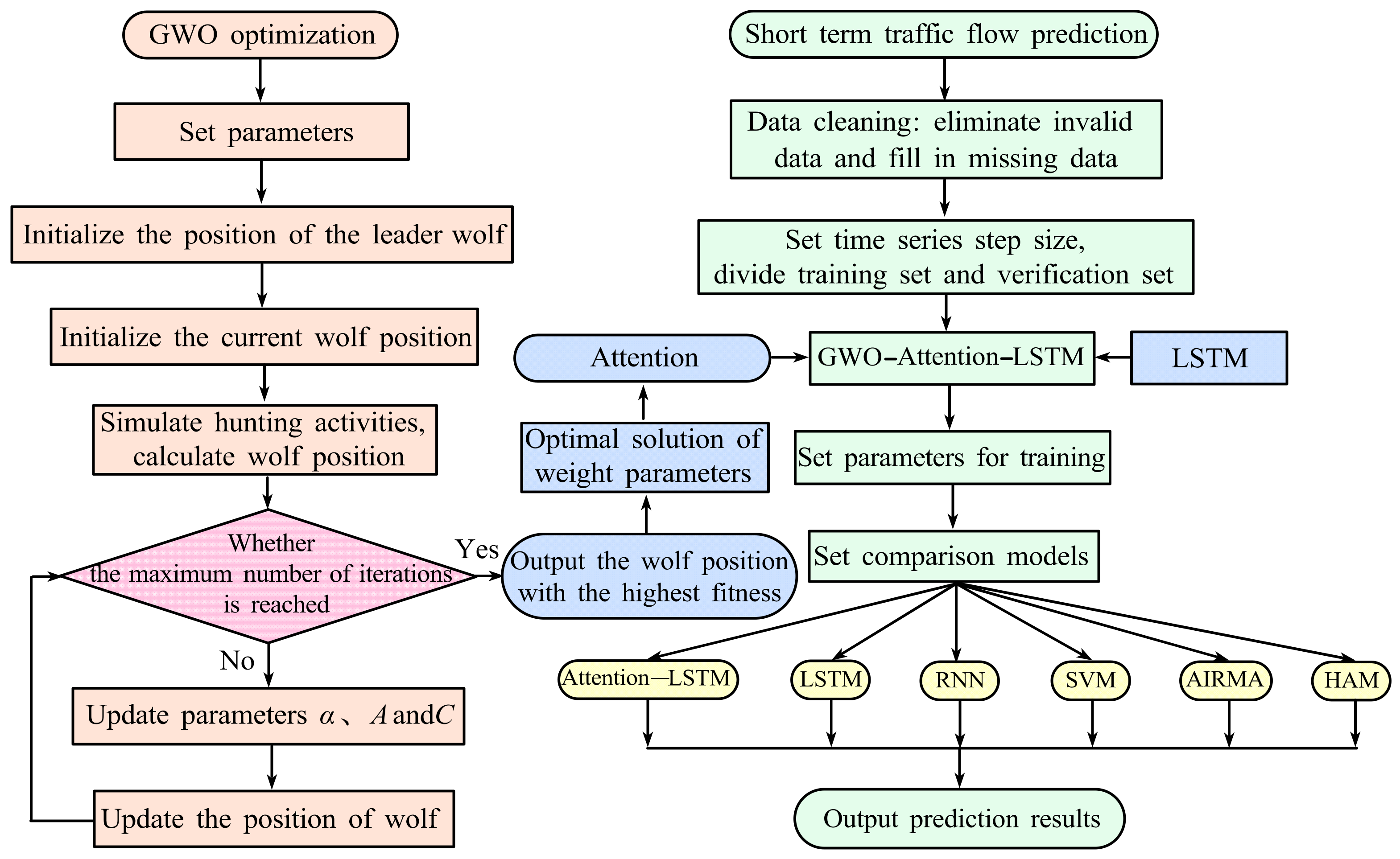
Short-term traffic flow prediction steps based on the GWO-Attention-LSTM model are shown in Figure 1. The main body-prediction process of the model is the flow chart on the right. Firstly, the collected traffic flow data is cleaned, and the basic parameters are set. Secondly, the attention mechanism is added to the LSTM model, and training parameters of all comparison models are set. Finally, the prediction results are output. The optimization process of the model is the flow chart on the left. Firstly, set the relevant parameters of the GWO algorithm. The position of the leader wolf and other wolves is initialized. Secondly, the hunting process is simulated, and the relevant parameters are updated to calculate the fitness value of wolves. Finally, when the maximum number of iterations is reached, the wolf position with the best fitness is output as the optimal initial value parameter of the attention mechanism.

3.1. LSTM Combined with Attention Mechanism

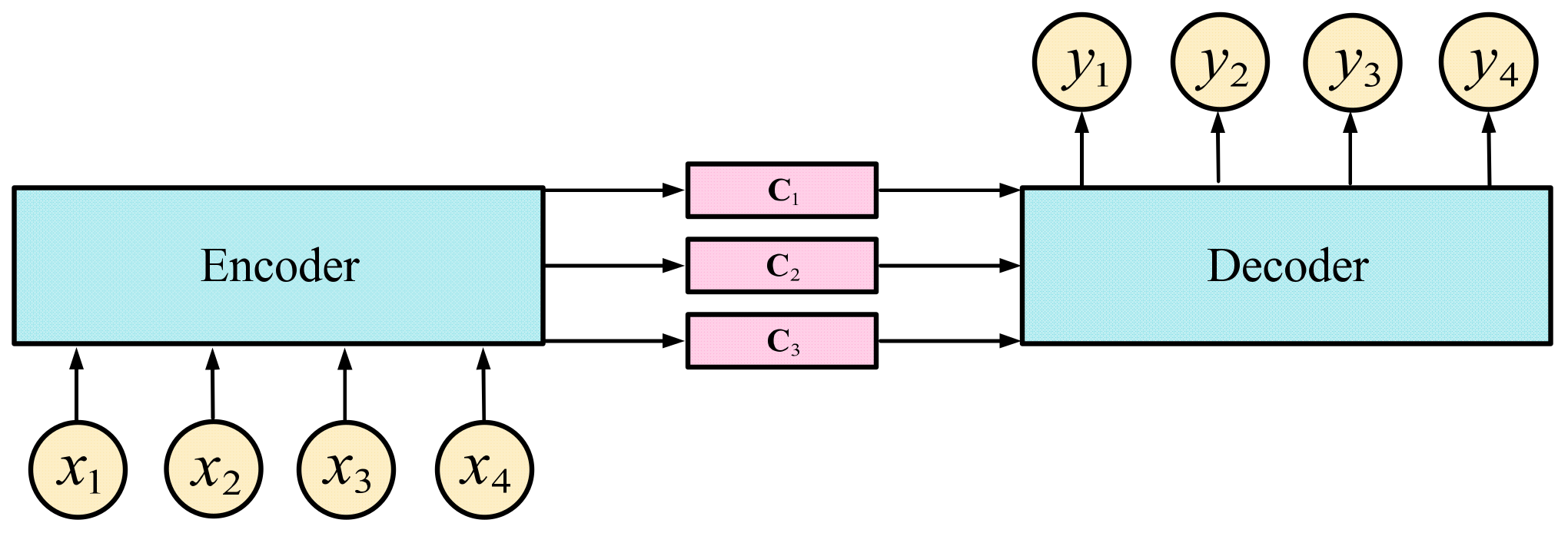
The attention mechanism originates from the human brain’s attention. Moreover, the attention mechanism usually appears in the encoder–decoder structure [28]. The encoder-decoder contains two types of RNN networks, which are used for decoding and encoding, respectively. The encoder can encode the input information and convert the input value into an intermediate value containing information features. The decoder will decode the intermediate value to obtain the processing result.

As shown in Figure 2, the attention mechanism is added to the encoder–decoder structure. In the process of encoding and decoding, the attention mechanism allocates weights and sums them according to the importance of different information elements. Therefore, the attention mechanism can help the model judge the importance of different information in the sequence, and improve the weight of important information, so as to improve the learning efficiency of the model. The result of weighting and summing feature information by the attention mechanism is $C={\displaystyle \sum _{n=1}^M{\alpha }_n{e}_n}$. In equation: ${\alpha }_n$ is the weight value; $e_n$ is the hidden value of the encoder part; $M$ is the number of hidden values.

The LSTM network can selectively retain and forget historical information. Compared with the RNN network, the LSTM network can effectively solve the problem of long-term dependence [29]. However, the LSTM network will continuously accumulate path branches of previous unit forgetting and memory. As the time span of the input sequence increases, the path structure of the network becomes more and more complex, which limits the performance of the model. At this time, it is necessary to optimize the learning mode of the model for feature information, select important units to extract information for full learning, and reduce the attention to low impact information.

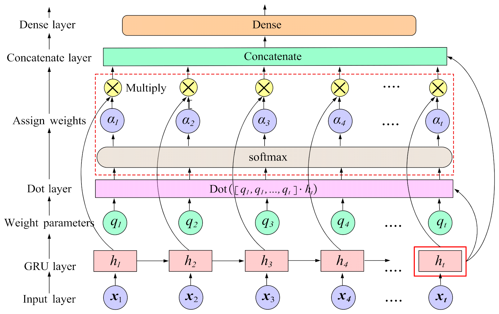
Therefore, in order to improve the performance of the model, the attention mechanism is added to the LSTM model. As shown in Figure 3, after the input values $\left[x_1,x_2,x_3,\dots ,x_t\right]$ are extracted from the LSTM network information, the feature information $\left[h_1,h_2,h_3,\dots ,h_t\right]$ in each step is obtained. The initial weight parameters are set as $\left[q_1,q_2,q_3,\dots ,q_t\right]$. Parameter $q_t$ of weight ${\alpha }_t$ is adjusted during model iteration.

In order to improve the dependence of the weight assigned by the attention mechanism on the final information extraction result of LSTM, each initial calculated weight parameter $\left[q_1,q_2,q_3,\dots ,q_t\right]$ is compared with the information extraction result $h_t$ of the last time step of LSTM. Furthermore, this paper uses the activation function $softmax$ to convert the calculated result into a weight score to measure the importance of information. The calculation process of weight $\left[{\alpha }_1,{\alpha }_2,\dots ,{\alpha }_t\right]$ is shown in Equation (1).

$$[{\alpha }_1,{\alpha }_2,\dots ,{\alpha }_t]=softmax([q_1,q_2,\dots ,q_t]\cdot h_t)$$

(1)

This paper multiplies the calculated weight value with the information extraction result of each step of the LSTM layer to complete the weight distribution and summation. Their calculation process is shown in Equation (2). The attention mechanism strengthens the weight of important information, making the model no longer blindly learn, but instead focus on mining feature information according to important information. In this way, the model can more easily capture the deep rules hidden in the time series. Finally, the weight summation result $C$ is sent to the dense layer to obtain the predicted value.

$$C={\displaystyle \sum _{t=1}^T{\alpha }_t\cdot h_t}$$

(2)

In Equation (2): $T$ is the length of the time step.

In the figure: $x_t$ is the input value; $h_t$ is the feature extraction value of the LSTM layer at time $t$; $q_t$ is the calculation parameter of weight; ${\alpha }_t$ is the weight assigned to the attention mechanism.

3.2. Model Optimization Based on GWO Algorithm

3.2.1. Grey Wolf Optimizer Algorithm

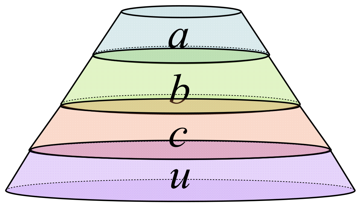
The grey wolf optimizer (GWO) is an optimization algorithm established by Mirjalili et al. [30]. They proposed this algorithm by observing the hunting activities of wolves. This optimization algorithm has fewer parameters. The GWO has the advantages of strong generalization and optimization ability. The core idea of the GWO algorithm is to simulate the social relationship and hunting behavior of wolves, and find the optimal hunting position of gray wolves of different levels by constantly adjusting parameters. As shown in Figure 4, the social relations of wolves have four levels. The first level is set as wolf $a$, which belongs to the leader wolf. It is responsible for leading the wolves to find prey, chasing and suppressing prey, and the rest of gray wolves must obey the decision of wolf $a$. The second level is set as wolf $b$. Its task is to assist wolf $a$ and command the remaining wolves except wolf $a$. The third level is set as wolf $c$, which needs to follow the management of the above two levels of gray wolves and manage the gray wolves of lower social levels. The fourth level is set as wolf $u$. Wolf $u$ is the lowest-level gray wolf in the society and follows the command of gray wolves at all levels above.

According to the above social hierarchy, wolves hunt under the command of the highest-level gray wolves. The hunting process simulated using the GWO algorithm is as follows:

Suppose the number of wolves is $l$, the distance between gray wolves and their prey is $H$. The process of wolves searching for their prey and constantly approaching their prey is shown in Equation (3).

$$\left\{\begin{array}{c}H=\left|C\cdot X_R\left(k\right)-X_i\left(k\right)\right|\\ X_i\left(k+1\right)=X_R\left(k\right)-A\cdot H\end{array}\right.$$

(3)

In Equation (3): $k$ is the number of iterations; $X_i\left(k\right)$ represents the position of gray wolf $i$ after $k$ iterations; $X_R\left(k\right)$ is the position of prey after $k$ iterations; $X_i\left(k+1\right)$ is the position of gray wolf regeneration; $A$ and $C$ are coefficient vectors. Their calculation is shown in Equation (4).

$$\left\{\begin{array}{c}A=2\alpha (r_1-1)\\ C=2r_2\end{array}\right.$$

(4)

In Equation (4): $r_1$ and $r_2$ is a random number between zero and one; $\alpha$ is the convergence factor, reduced from two to zero.

In the $d$ dimensional space, the position of wolf $a$ is set to $X_a\left(X_{a,1},X_{a,2},\dots ,X_{a,d}\right)$; the position of wolf $b$ is set to $X_b\left(X_{b,1},X_{b,2},\dots ,X_{b,d}\right)$; the position of wolf $c$ is set to $X_c\left(X_{c,1},X_{c,2},\dots ,X_{c,d}\right)$. Under the leadership of wolf $a$, wolf $b,$ and wolf $c$, the wolves can find and surround the prey. The position update process of other gray wolves is shown in Equations (5)–(7).

$$\left\{\begin{array}{c}{H}_a=\left|C_1\cdot X_a(k)-X_i\left(k\right)\right|\\ H_b=\left|C_2\cdot X_b(k)-X_i\left(k\right)\right|\\ H_c=\left|C_3\cdot X_c(k)-X_i\left(k\right)\right|\end{array}\right.$$

(5)

$$\left\{\begin{array}{c}{X}_{i,a}(k+1)=X_a(k)-A_1{H}_a\\ X_{i,b}(k+1)=X_b(k)-A_2{H}_b\\ X_{i,c}(k+1)=X_c(k)-A_3{H}_c\end{array}\right.$$

(6)

$$X_i(k+1)=\frac{X_{i,a}+X_{i,b}+X_{i,c}}{3}$$

(7)

In the above Equations (5)–(7): $H_a$, $H_b$ and $H_c$ are the distances between wolf $a$, wolf $b,$ and wolf $c$ with the current wolf $X_i\left(k\right)$; $X_{i,a}\left(k+1\right)$ is the updated position of wolf $i$ under the leadership of wolf $a$; $X_{i,b}\left(k+1\right)$ is the updated position of wolf $i$ under the leadership of wolf $b$; $X_{i,c}\left(k+1\right)$ is the updated position of wolf $i$ under the leadership of wolf $c$; $X_i\left(k+1\right)$ is the updated position of wolf $i$ under the leadership of wolf $a$, wolf $b,$ and wolf $c$.

3.2.2. Optimization Process of GWO Algorithm

The attention mechanism can improve model performance. However, the initial weight parameter $q_t$ of the attention mechanism is a random value. It is adjusted in the iterative process according to the training parameters set by the model. Therefore, the weight value allocated for each training cannot be guaranteed to be the optimal result. This paper considers using the strong optimization ability of the GWO algorithm to optimize the initial weight parameter $q_t$.

Firstly, this paper builds the LSTM model and adds the attention mechanism. This step sets learning rate, number of neurons, activation function, and other parameters.

Secondly, the position of the wolves is initialized. This step sets the number of wolves, search space dimension, value range of position parameter, and maximum number of iterations.

This paper simulates the hunting activities of wolves to obtain the fitness of each gray wolf. The top three individuals with fitness are set to wolf $a$, $b,$ and $c$. Under the leadership of wolf $a$, wolf $b,$ and wolf $c$, the current position of wolf $i$ is updated.

The satisfaction of the maximum number of iterations is judged. If the number of iterations does not satisfy the requirements, the parameters $\alpha ,A$ and $C$ will be updated. In this case, the fitness ranking of gray wolves will be recalculated, and the position of the gray wolves will be updated. If the maximum number of iterations is reached, the position $X_a\left(X_{a,1},X_{a,2},\dots ,X_{a,d}\right)$ with the highest fitness ranking is mapped to the optimal solution of the weight parameter matrix $\left[q_1,q_2,q_3,\dots ,q_t\right]$. The number of position components of the best gray wolf $a$ is consistent with the step size of the time series, so the optimal initial weight parameter matrix is $\left[X_{a,1},X_{a,2},\dots ,X_{a,t}\right]$. The weight conversion process of the attention mechanism is shown in Figure 5.

Finally, the optimal weight parameters are input into the attention mechanism. The final information extraction result of LSTM is set as $\overline{h}$. The initial weight summation result of the optimized attention mechanism is shown in Equation (8). According to the above process, the model optimization based on the GWO algorithm is realized.

$$C^{\prime }={\displaystyle \sum _{t=1}^{T}softmax(X_{a,t}\cdot \overline{h})\cdot h_t}$$

(8)

4. Simulation and Analysis of Experiment

4.1. Experimental Data

Four trunk roads in Qingdao (China) are selected as the research objects. The four trunk roads are representative and conform to the characteristics of typical urban roads in China. The data acquisition method is to view the vehicle information captured and recorded by the monitoring camera on the trunk road. The research group counts the number of license plate numbers every 5 min. A total of 41 days of traffic flow data are eventually collected. The relevant information of each road section is shown in

Table 2. Information about trunk roads.

Name	Collection Time	Number of Lanes	Maximum Traffic Flow (veh/5 min)	Data Volume	Repaired Data	Location
Jilan Road	1 July 2021–11 August 2021	6	81	11,808	23	Near the suburb
Qingwei Road	1 July 2021–11 August 2021	8	145	11,808	41	Near the school
Mocheng Road	1 July 2021–11 August 2021	6	169	11,808	35	Near the mall
Haier Road	1 July 2021–11 August 2021	6	122	11,808	31	Near the viaduct

.

The system used for data collection has a very low probability of error, therefore, the data need to be checked and cleaned. This paper sets the circular function to find ‘space’, ‘letter’, or ‘punctuation’ in the data. Because the amount of data used in this paper is large enough, replacing a small number of outliers has little impact on the prediction results, considering that the value of traffic flow changes gradually with time. Therefore, this paper replaces the outlier with the average of two normal values near the outlier. The valid data range is set. The data beyond the set range is replaced by the average value.

Table 3. Example of input data.

Time	Jilan Road (veh/5 min)	Qingwei Road (veh/5 min)	Mocheng Road (veh/5 min)	Haier Road (veh/5 min)
1 July 2021 00:00:00	4	10	22	5
1 July 2021 00:05:00	4	18	16	10
1 July 2021 00:10:00	5	14	17	7
1 July 2021 00:15:00	6	10	18	5

shows some examples of relevant input data after cleaning.

4.2. Evaluation Metrics and Parameter Setting of the Prediction Model

Evaluation metrics of the prediction models are as follows:

Mean absolute error (MAE) is shown in Equation (9).

$$\mathrm{MAE}=\frac{1}{m}{\displaystyle \sum _{i=1}^m\left|\left(y_i-{\widehat{y}}_i\right)\right|}$$

(9)

Root mean square error (RMSE) is shown in Equation (10).

$$\mathrm{RMSE}=\sqrt{\frac{1}{m}{\displaystyle \sum _{i=1}^m{\left(y_i-{\widehat{y}}_i\right)}^2}}$$

(10)

Average absolute percentage error (MAPE) is shown in Equation (11).

$$\mathrm{MAPE}=\frac{100\%}{m}{\displaystyle \sum _{i=1}^m\left|\frac{{\widehat{y}}_i-y_i}{y_i}\right|}$$

(11)

In the above Equations (9)–(11): $m$ is the number of samples; $y_i$ is the actual traffic flow value at time $i$; and ${\widehat{y}}_i$ is the predicted value of traffic flow at time $i$.

The algorithms involved in this paper are based on the Python language environment. The central processing unit (CPU) of the computer is the AMD-5800H. The graphics processing unit (GPU) of the computer is the RTX3050. The comparison models are set as: the attention-LSTM model, LSTM model, RNN model, SVM model, ARIMA model, and HAM model. In the experiment, the learning rate of all neural network models is set to 0.0001, and the batch size is set to 128. Adaptive moment estimation (ADAM) is used as the optimizer of the model. The MSE is taken as the loss function of the model. The ratio of training set and verification set is set to 7:1. The number of training iterations is set to 300. To ensure that the model can fully explore the features of the input sequence, the input value of the model is 120 min of traffic flow ($24\times 5=120 \min$). The early stopping is set to 20. If the MSE does not decline for 20 consecutive sequences, the model will stop training and save the optimal model.

The parameters of the SVM model are set as follows: the penalty coefficient $C$ of the objective function is 1; the gamma value is 0.1; the kernel-function is set to $rbf$. This paper uses the SVM-branch support vector regression (SVR) to predict. The expression of SVR is shown in Equation (12).

$$f(x)={\displaystyle \sum _{i=1}^n(\widehat{{\alpha }_i}-{\alpha }_i)}\kappa (x_i^T{x}_i)+b$$

(12)

where: $\widehat{{\alpha }_i}$ and ${\alpha }_i$ are $Lagrangian$ coefficients; kernel function $\kappa \left(x_i^T{x}_i\right)=e^{(-\frac{{\Vert x_i-x_j\Vert }^2}{2{\sigma }^2})}$, $\sigma >0$.

The LSTM and RNN neurons in the experimental model are set to 128, and the activation function is set to $tanh$. The wolf group $l$ of the GWO algorithm is set to 20, the maximum number of iterations is set to 50. The weight parameter value range is $\left[-1,1\right]$. The dimension $d$ of the search space is set to 24. All comparison models are debugged to the best state. The selection process of important hyperparameters is as follows:

(1) The LSTM network needs to determine the time step. The choice of time step will affect the efficiency of model learning. Therefore, time steps of 6, 12, 24 and 36 are set respectively for training. Taking one of the roads as an example, the prediction errors of different time steps are shown in

Table 4. The prediction errors of different time steps.

Time Step	MAE	RMSE	MAPE (%)
6	2.8075	4.1123	26.87
12	2.7636	3.9982	26.25
24	2.6783	3.8402	25.82
36	2.7241	3.8933	25.94

. It can be seen that the model has the lowest error when the time step is 24.

(2) The number of layers and neurons of the LSTM network will determine the depth of the model. In general, the more layers and neurons of LSTM, the more precise the model is. However, the model proposed in this paper adds a deeper-network attention mechanism. When the depth of LSTM is too large, it will increase the training burden of the model. As shown in

Table 5. The prediction errors of different layers and neurons.

Layers	Neurons	MAE	RMSE	MPAE (%)
1	64	2.8819	3.9543	27.13
	128	2.6783	3.8402	25.82
	256	2.7125	3.8842	26.46
2	64	2.8717	3.9104	26.68
	128	2.8821	3.9245	27.12
	256	2.8903	3.9755	27.36
3	64	2.8933	3.9778	27.41
	128	2.8725	3.9588	27.69
	256	2.9011	3.9982	28.46

, the previous analysis confirmed that when the number of the LSTM layers is one, the performance of the model is good. When the number of LSTM neurons is 128, the error of the model is the lowest.

4.3. Analysis of Prediction Results

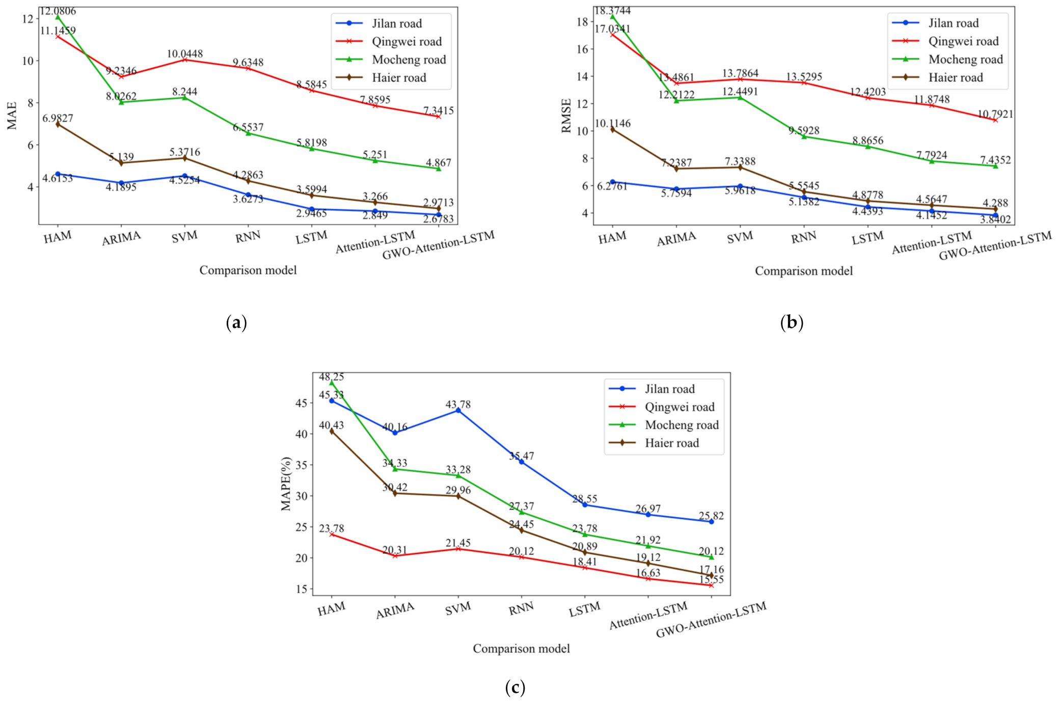
The GWO-attention-LSTM, attention-LSTM model, LSTM model, RNN model, SVM model, ARIMA model, and HAM model are trained respectively. The comparison of prediction errors of all models is shown in Figure 6.

From Figure 6, it can be seen that the GWO-attention-LSTM model has better prediction results compared to other models. The following results are obtained:

(1) In the four road sections, the MAE value of the GWO-attention-LSTM model decreased by 38.34%, 34.53%, and 48.32% on average compared with the SVM model, ARIMA model, and HAM model; the RMSE value decreased by 34.79%, 33.29%, and 48.15% on average; the MAPE value decreased by 37.70%, 36.03%, and 48.38% on average. It can be seen that the GWO-attention-LSTM model has a substantial improvement in accuracy compared with the traditional prediction models.

(2) In the four road sections, the MAE value of the GWO-attention-LSTM model decreased by 26.60% on average compared with the RNN model; the RMSE value decreased by 22.70% on average; the MAPE value decreased by 26.56% on average. Therefore, it can be proved that the GWO-attention-LSTM model has obvious advantages over the traditional recurrent neural network.

(3) In the four sections, the MAE value of the GWO-attention-LSTM model decreased by 7.32% and 14.35% on average compared with the attention-LSTM model and LSTM model; the RMSE value decreased by 6.78% and 13.71% on average; the MAPE value decreased by 7.31% and 14.59% on average. It can be seen that the attention mechanism can significantly improve the prediction accuracy of the the LSTM model. Moreover, because the GWO algorithm optimizes the parameters of the initial weights, the model can find the relatively important feature information in the time series more accurately. Therefore, the prediction error of the GWO-attention-LSTM model is lower compared with other models. In addition, the GWO-attention-LSTM model has a very low prediction error for predicting four road sections with different zone conditions under the same training parameter settings, which proves the applicability and portability of the model.

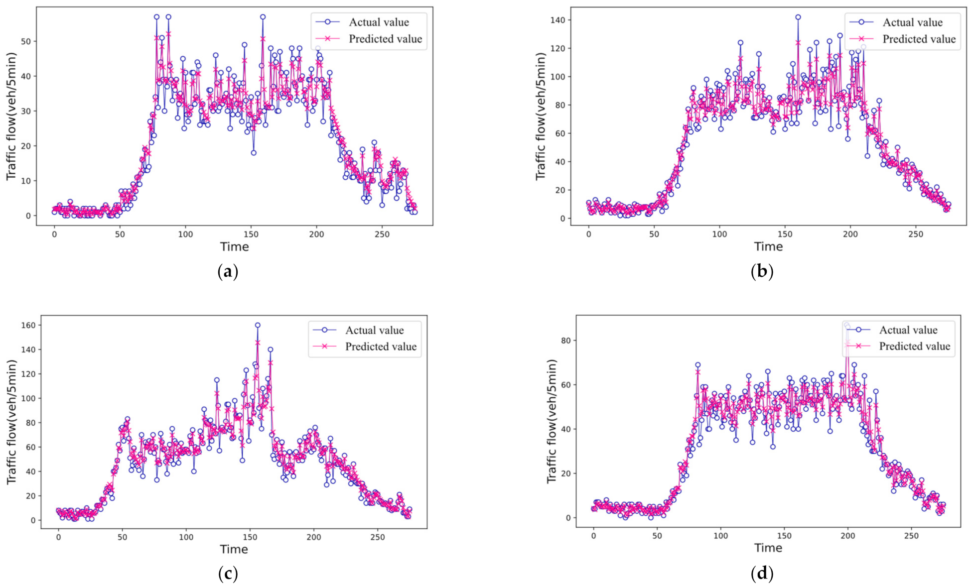
As shown in Figure 7, the prediction results of the GWO-attention-LSTM model are compared with the actual values. It can be seen that the GWO-attention-LSTM model accurately predicts the trend of the actual traffic flow time series. The polyline of the GWO-attention-LSTM model is more consistent with the actual value polyline. In addition, the prediction points are highly close to the top of several actual points. Therefore, it is proved that the GWO-attention-LSTM model has good nonlinear fitting ability.

4.4. Optimization Analysis

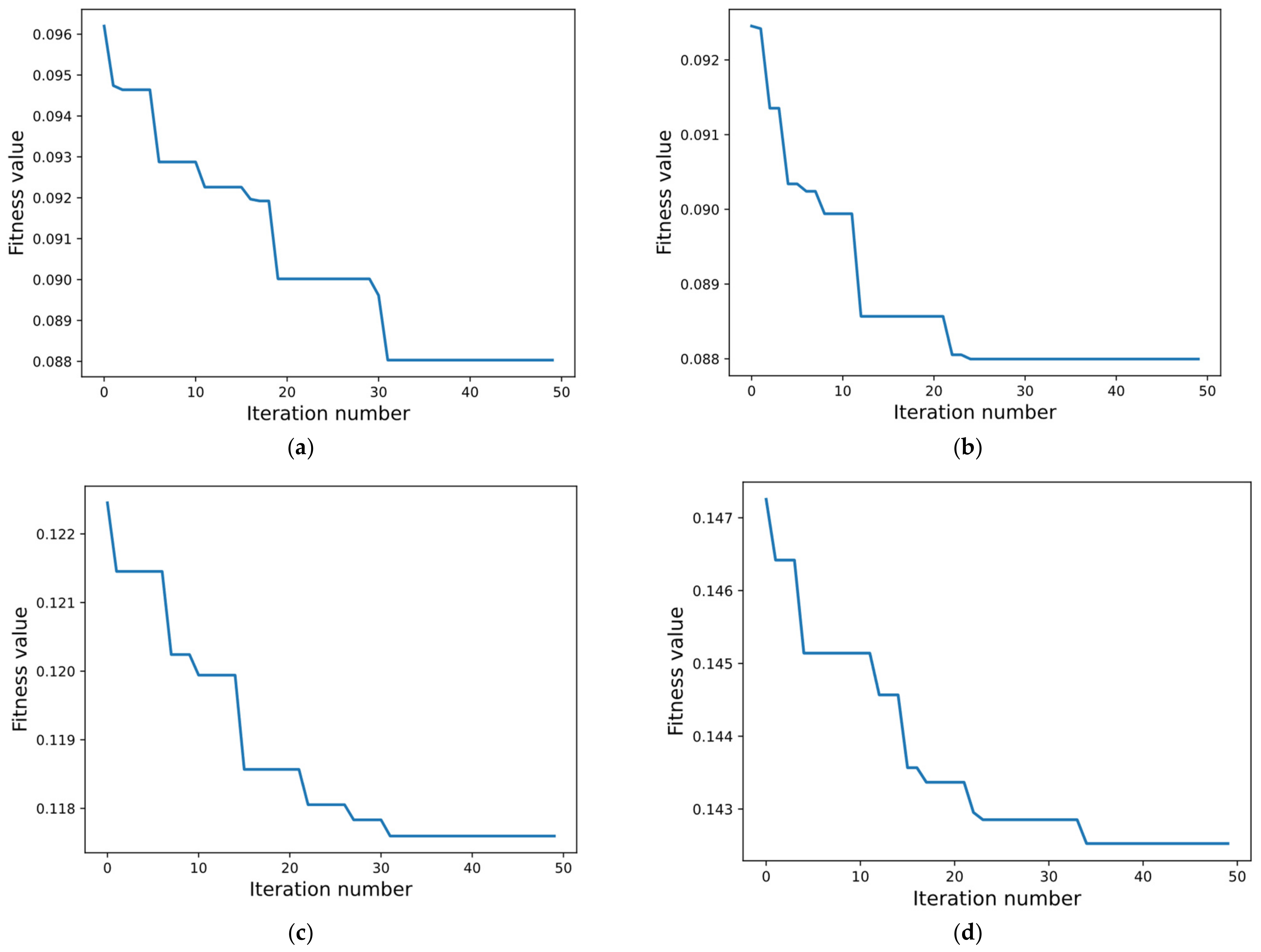
The GWO algorithm continuously approaches and surrounds the target prey by updating the hunting position of the wolf during the iterations. The change process of the iteration number and fitness value of the wolf $a$ is shown in Figure 8. It can be seen that the fitness value of Jilan Road is stable at 0.09002 after the 31st iteration. The fitness value of Qingwei Road is stable at 0.08805 after the 25th iteration. The fitness value of Mocheng Road is stable at 0.09261 after the 33rd iteration. The fitness value of Haier Road is stable at 0.14285 after the 35th iteration. The above results show that the GWO algorithm has the advantages of fast convergence and high applicability. In addition, the best adapted wolf can be obtained quickly for all road sections, so as to obtain the optimal initial weight parameters for the attention mechanism.

In this paper, early stopping is set in the training process, and this method can effectively avoid overfitting. The earlier the model jumps out of training, the better the actual performance of the model. As shown in Figure 9, the number of training iterations and the loss value curves of the GWO-attention-LSTM model, attention-LSTM model, and LSTM model are compared. It can be seen that the number of iterations of both the GWO-attention-LSTM model and the attention-LSTM model are significantly reduced compared to the LSTM model. Among them, the GWO-attention-LSTM model has the least number of training iterations and the fastest decrease in the loss value MSE. It can be seen that the attention mechanism increases the weight of important feature information, and the model can capture the hidden patterns in the time series faster. Moreover, because the GWO algorithm optimizes the initial weight parameters, the attention mechanism can calculate the appropriate weight values faster and more accurately. Therefore, the GWO-attention-LSTM model has better model performance compared with other prediction models.

5. Conclusions

In order to make the model more accurate and easier to be trained, a short-term traffic flow prediction model based on the GWO-attention-LSTM is constructed. The attention mechanism is added on the basis of the LSTM network. Through the attention mechanism, the weight of important information is enhanced, so as to improve the feature learning ability of the model. This paper considers the lack of research on the optimization of the attention mechanism. Therefore, this paper uses the GWO algorithm to optimize the initial weight parameters of the attention mechanism. This optimization algorithm enables the model to converge quickly, which improves the performance of the model.

The prediction effect of the GWO-attention-LSTM model is verified via the simulation of actual data. Traffic flow data of several trunk roads in Qingdao (China) are collected for simulation analysis. The experimental results show that the prediction error of the GWO-attention-LSTM model is significantly lower than that of the LSTM model. In addition, the accuracy of the GWO-attention-LSTM model is significantly improved compared with the mainstream machine learning models and recurrent neural network models. In addition, the GWO-attention-LSTM model proves to be easier to be trained through a model optimization analysis.

However, the model proposed in this paper still has shortcomings. The GWO-attention-LSTM model is less effective in long-term traffic flow prediction. The main reasons are that the model considers too few relevant factors and that the amount of data is not large enough. Therefore, subsequent research will build the database with a larger time span and collect more relevant data for research.

References

1. Zhang, H.; Dai, G.L. The strategy of traffic congestion management based on case-based reasoning. Int. J. Syst. Assur. Eng. Manag. 2019, 10, 142–147. [Google Scholar] [CrossRef]
2. Tripathi, P.S.M.; Kumar, A.; Chandra, A. An overview of intelligent transport system (ITS) and ITS applications. J. Mob. Multimed. 2021, 17, 79–114. [Google Scholar] [CrossRef]
3. Dharyll, P.M.A. Short-term traffic flow forecasting using the autoregressive integrated moving average model in Metro Cebu (Philippines). Int. J. Appl. Decis. Sci. 2021, 14, 565–587. [Google Scholar]
4. Dahui, L.I. Predicting short-term traffic flow in urban based on multivariate linear regression model. J. Intell. Fuzzy Syst. 2020, 39, 1417–1427. [Google Scholar]
5. Vladimir, D.; Vladimir, M.; Krasnova, I. Traffic flows forecasting based on machine learning. Int. J. Embed. Real-Time Commun. Syst. (IJERTCS) 2022, 13, 1–19. [Google Scholar]
6. Reshma, R.N.; Rajabhushanam, C. Machine learning algorithms performance evaluation in traffic flow prediction. Mater. Today Proc. 2022, 51, 1046–1050. [Google Scholar] [CrossRef]
7. Monal, P.; Carlos, V.; Arvind, Y. Metaheuristic enabled deep convolutional neural network for traffic flow prediction: Impact of improved lion algorithm. J. Intell. Transp. Syst. 2022, 26, 730–745. [Google Scholar]
8. Shi, R.Z.; Du, L.J. Multi-section traffic flow prediction based on MLR-LSTM neural network. Sensors 2022, 22, 7517. [Google Scholar] [CrossRef]
9. Zhao, C.; Liu, R.; Su, B.; Zhao, L.; Han, Z.; Zheng, W. Traffic flow prediction with Attention mechanism based on TS-NAS. Sustainability 2022, 14, 12232. [Google Scholar] [CrossRef]
10. Li, M.; Li, M.; Liu, B.; Liu, J.; Liu, Z.; Luo, D. Spatio-temporal traffic flow prediction based on coordinated attention. Sustainability 2022, 14, 7394. [Google Scholar] [CrossRef]
11. He, G.G.; Li, Y.; Ma, S.F. Discussion on short-term traffic flow prediction method based on mathematical model. Syst. Eng. Theory Pract. 2000, 20, 51–56. [Google Scholar]
12. Williams, B.M.; Hoel, L.A. Modeling and forecasting vehicular traffic flow as a seasonal ARIMA process: Theoretical basis and empirical results. J. Transp. Eng. 2003, 129, 664–672. [Google Scholar] [CrossRef] [Green Version]
13. Clark, S. Traffic prediction using multivariate nonparametric regression. J. Transp. Eng. 2003, 129, 161–168. [Google Scholar] [CrossRef]
14. Xiong, T.; Qi, Y.; Zhang, W.B. Short-term traffic flow prediction based on DCLSTM-RF model for road network. Comput. Sci. 2020, 47, 84–89. [Google Scholar]
15. Zou, Z.M.; Hao, L.; Li, Q.J.; Chen, H.; Kang, L. Expressway short-term traffic flow prediction based on particle swarm optimization support vector regression. Sci. Technol. Eng. 2021, 21, 5118–5123. [Google Scholar]
16. Lin, G.; Lin, A.; Gu, D. Using support vector regression and K-nearest neighbors for short-term traffic flow prediction based on maximal information coefficient. Inf. Sci. 2022, 608, 517–531. [Google Scholar] [CrossRef]
17. Yao, B.; Ma, A.; Feng, R.; Shen, X.; Zhang, M.; Yao, Y. A deep learning framework about traffic flow forecasting for urban traffic emission monitoring system. Front. Public Health 2022, 9, 804298. [Google Scholar] [CrossRef]
18. Wang, M.Z.; Ai, X.H.; Qin, K.H.; Huang, H. Traffic flow prediction model of BP neural network based on adaptive genetic algorithm optimization. Adv. Appl. Math. 2020, 9, 1317–1326. [Google Scholar] [CrossRef]
19. Chen, X.P.; Zeng, S.; Hu, G. Short term traffic flow prediction based on BP neural network. Highw. Traffic Technol. 2008, 3, 115–117. [Google Scholar]
20. Hochreiter, S.; Schmidhuber, J. Long short-term memory. Neural Comput. 1997, 8, 1735–1780. [Google Scholar] [CrossRef]
21. Ma, X.; Tao, Z.; Wang, Y.; Yu, H.; Wang, Y. Long short-term memory neural network for traffic speed prediction using remote microwave sensor data. Transp. Res. Part C 2015, 54, 187–197. [Google Scholar] [CrossRef]
22. Cao, B.; Gao, M.T. Research on short-term traffic flow prediction based on LSTM. Mod. Comput. (Prof. Ed.) 2018, 25, 3–7. [Google Scholar]
23. Zhong, C.H.; Wang, M.; Zhao, W.; Zhang, Y. Short term traffic flow prediction of intersection based on LSTM. Highw. Traffic Technol. 2019, 35, 6. [Google Scholar] [CrossRef]
24. Li, M.M.; Lei, J.Y.; Zhao, C.J. Short term traffic flow prediction based on LSTM-BP combination model. Comput. Syst. Appl. 2019, 28, 5. [Google Scholar]
25. Wang, P.X.; Zhang, Y.; Hu, T.; Zhang, T. Urban traffic flow prediction: A dynamic temporal graph network considering missing values. Int. J. Geogr. Inf. Sci. 2022. [Google Scholar] [CrossRef]
26. Chen, X.; Sun, L. Bayesian temporal factorization for multidimensional time series prediction. IEEE Trans. Pattern Anal. Mach. Intell. 2021, 44, 4659–4673. [Google Scholar] [CrossRef]
27. Wang, P.; Zhang, T.; Zheng, Y.; Hu, T. A multi-view bidirectional spatiotemporal graph network for urban traffic flow imputation. Int. J. Geogr. Inf. Sci. 2022, 36, 1231–1257. [Google Scholar] [CrossRef]
28. Ogura, T.; Magassouba, A.; Sugiura, K.; Hirakawa, T.; Yamashita, T.; Fujiyoshi, H.; Kawai, H. Alleviating the burden of labeling: Sentence generation by attention branch Encoder-Decoder network. IEEE Robot. Autom. Lett. 2020, 5, 5945–5952. [Google Scholar] [CrossRef]
29. Durand, D.; Aguilar, J.; Rmoreno, M.D. An analysis of the energy consumption forecasting problem in smart buildings using LSTM. Sustainability 2022, 14, 13358. [Google Scholar] [CrossRef]
30. Mirjalili, S.; Mirjalili, S.M.; Lewis, A. Grey wolf optimizer. Adv. Eng. Softw. 2014, 69, 46–61. [Google Scholar] [CrossRef]
Figure 1. Short-term traffic flow prediction steps are based on GWO-attention-LSTM.
Sustainability 15 01374 g001
Figure 2. Encoder-decoder combines with attention mechanism.
Sustainability 15 01374 g002
Figure 3. LSTM combines with attention mechanism.
Sustainability 15 01374 g003
Figure 4. Social class of gray wolves.
Sustainability 15 01374 g004
Figure 5. The weight conversion process of attention mechanism.
Sustainability 15 01374 g005
Figure 6. The comparison of prediction errors of all models. (a) MAE. (b) RMSE. (c) MAPE.
Sustainability 15 01374 g006
Figure 7. Comparison between predicted results and actual values. (a) Jilan Road. (b) Qingwei Road. (c) Mocheng Road. (d) Haier Road.
Sustainability 15 01374 g007
Figure 8. The change process of iteration number and fitness value. (a) Jilan Road. (b) Qingwei Road. (c) Mocheng Road. (d) Haier Road.
Sustainability 15 01374 g008
Figure 9. The number of training iterations and the loss value curves. (a) Jilan Road. (b) Qingwei Road. (c) Mocheng Road. (d) Haier Road.
Sustainability 15 01374 g009