Simplified Model for Concentration Analysis of Catalytic Conversion of Carbon Gas into Hydrogen

Abstract

The annual energy matrix has been changing in the last years because of the necessity of less dependence on fossil fuels, which are running out on the planet. Therefore, a study was begun to simulate the most efficient production of ${\mathrm{H}}_2$ through COMSOL Multiphysics^®, as it is a gas that in the future will be essential to supply the world’s energy necessities, due to it being easy to access and insert in gas pipes. From this study, we were able to present an optimization of parameters that presents good indications of how to obtain efficient hydrogen production in an idealized reactor.

1. Introduction

Since the beginning, humanity has been using different sources of energy for survival. In recent years, because of the high demand for petroleum-derived raw materials, the world has been concerned about the enormous amounts of pollutants released into the atmosphere by burning fossil fuels and the dependence on an energy source that may run out in the future.

Despite this enormous necessity to reduce the release of carbon gas into the atmosphere, the global energy matrix is still predominantly based on non-renewable sources. In order to fulfill the objectives of COP 21 (an agreement between 195 nations of the world to reduce the emissions of gases responsible for the greenhouse effect, with the aim of reducing global warming), the market for the use of natural gas has emerged as a competitive solution in the generation of less polluting energy for the planet [1].

Natural gas (NG) is a mixture of light hydrocarbons that remains in a gaseous state at normal temperature and pressure, and today generates more efficiency in the reduction of pollutants. In addition, in terms of world energy usage, its use has grown by about 38% per year. It is predominantly composed of ${\mathrm{CH}}_4$ and ${\mathrm{H}}_2$, mostly obtained from oil excavations [2].

As it is a fossil fuel, it is estimated that, in 40 or 50 years, NG reserves will have reached critical levels, and in Brazil, since 2019, an annual reduction of 10% of reserves has been observed. Considering highly efficient alternatives, countries in Europe and Brazil are studying the possibility of generating ${\mathrm{H}}_2$ to contribute to the natural gas originating from excavations, due to it being more efficient in the energy matrix [3].

${\mathrm{H}}_2$ can be obtained through numerous reactions, due to its easy connection with various chemical elements. One of the sources for obtaining this gas is by CO, a gas obtained through incomplete combustion of materials derived from carbon, for example, in car exhausts, through cigarette smoke, and coal burning in industries, among others [4]. In this project, we will simulate, through the COMSOL Multiphysics^® software, the most efficient way of producing this gas in a cylindrical reactor and pre-established conditions through the chemical equation:

$$\mathrm{CO}+{\mathrm{H}}_2\mathrm{O} \rightleftharpoons { \mathrm{H}}_2+{ \mathrm{CO}}_2$$

(1)

From reading scientific texts and previous numerical simulations, it was noted that the reverse reaction can be considered negligible in our analysis, which mainly aims to present a case study that analyzes the optimization, or the best composition, of three variables of the proposed case: inlet velocity, inlet concentration (${\mathrm{H}}_2\mathrm{O}$), and reactor geometry.

2. Chemistry Kinetic

Chemical kinetics studies the behavior of chemical reactions according to the time and rate (speed) at which they occur, with the objective of understanding their evolution at a macroscopic and microscopic level [5].

According to [5], there are many factors that interfere with the rate of a reaction, but we can mention four main ones: the physical state of the reactants, inlet concentrations, the temperature of the medium, and the presence or absence of a catalyst. Therefore, the rate of a general reaction can be given by:

$$rate=k{\left[reagent 1\right]}^m{\left[reagent 2\right]}^n$$

(2)

where:

• m and n make up the overall reaction order and are determined empirically;
• k is the speed constant.

The reaction rate constant depends on the collision energy of the molecules, their orientation, and the temperature of the medium. This relationship can be defined using the Arrhenius equation [6]:

$$k=A{e}^{\frac{-Ea}{RT}}$$

(3)

where k is the reaction rate constant, Ea is the activation energy of the reaction, R is the gas constant (R = 8.314 J/K·mol), T is the temperature in K, and A is the frequency of collisions that happen with correct geometry.

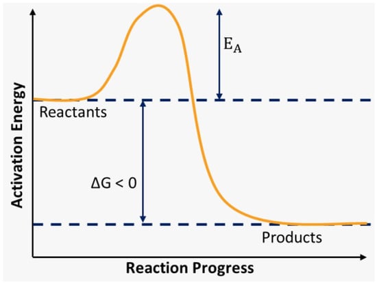
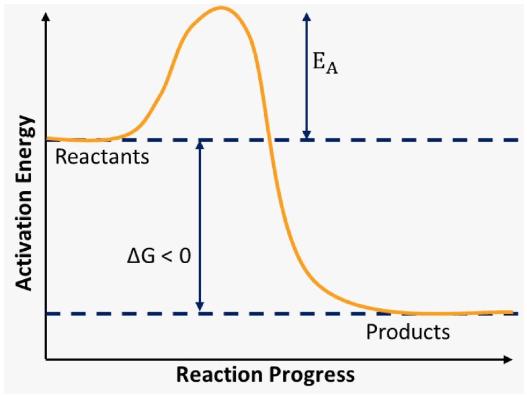
The activation energy is the minimum energy for the chemical reaction to occur; that is, for the bonds between the reactants to be broken and the new bonds between the products to be formed, as exemplified in Figure 1.

Figure 1. Exemplification of Activation Energy.

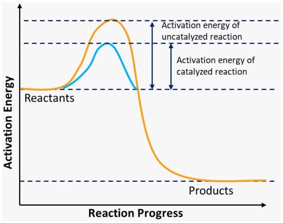
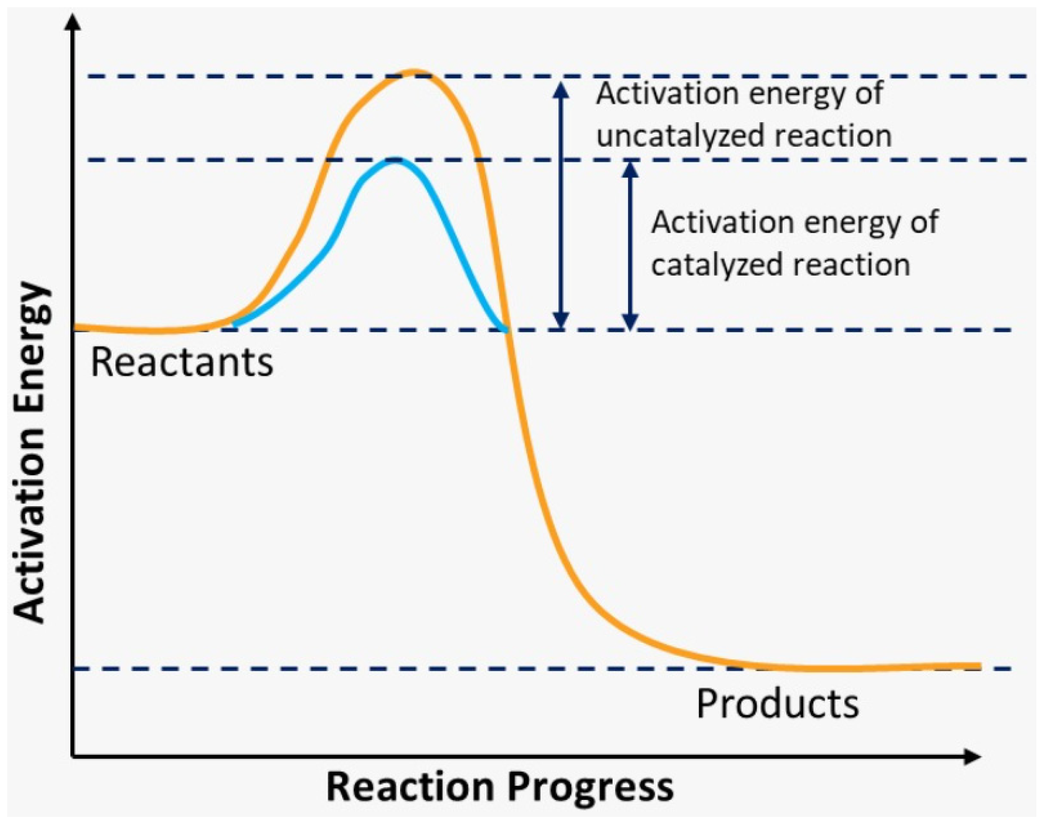
To increase the speed of the chemical reaction, we can use a catalyst, which is a substance capable of accelerating the process without undergoing changes; that is, it is not consumed and regenerates itself at the end of the reaction. The catalytic agent acts to reduce the activation energy of the reaction, as we can see in Figure 2 [7].

Figure 2. Reaction without and with the presence of catalyst.

Therefore, the lower the activation energy, the faster the reaction takes place, and vice versa.

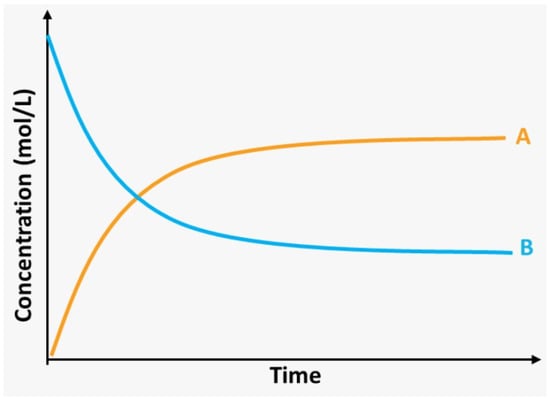
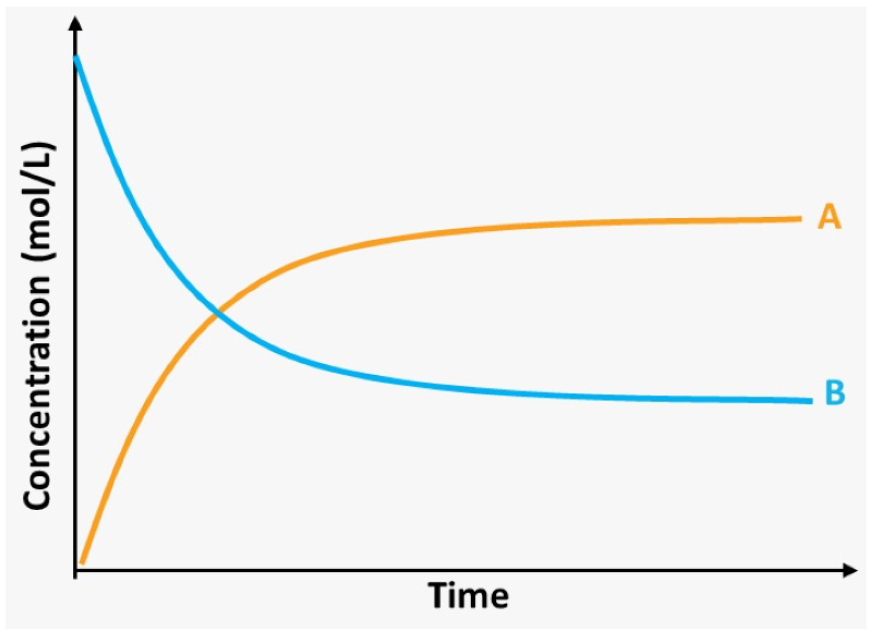
Finally, the last important topic to describe in this process is the concept of chemical equilibrium, which represents a dynamic state between two or more processes occurring at the same time and at the same speed [8].

Still according to [9], for the chemical equilibrium to be reached, it is necessary that the pressure and temperature of the reactor remain constant, in addition to the system being closed. With this, the concentrations remain constant over time, not changing while the environment is not changed, as we can see in Figure 3.

Figure 3. Chemical Equilibrium. A: reactantes; B: products.

3. Methodology

3.1. Parameters

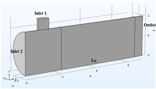
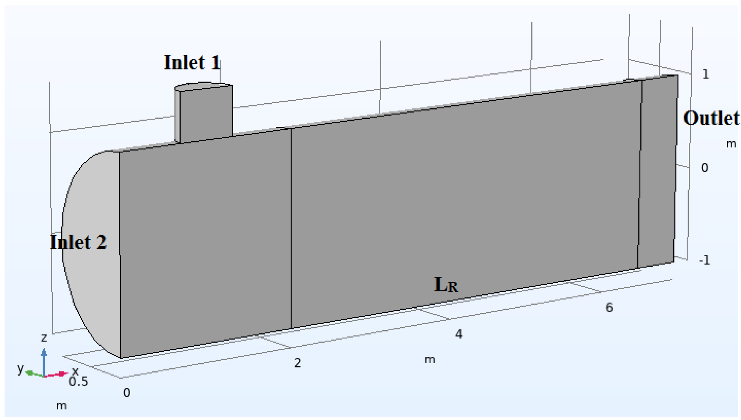
In order to analyze the influence and/or importance of the three parameters proposed here (inlet speed, reactor geometry, and inlet concentration), the reactor geometry is initially presented, as shown in Figure 4.

Figure 4. Reactor geometry.

Here, the following simplifications or considerations will be adopted:

• Due to the geometry of the reactor, symmetry in the $y=0$ plane will be considered;
• $\mathrm{CO}$ inlet concentration is equal to $10 \mathrm{mol}/{\mathrm{m}}^3$(Inlet 1) in all numerical simulations;
• Reactor diameter is equal to 1 m;
• The domain is entirely composed of air;
• The speeds at inputs 1 and 2 are the same;
• Isothermal analysis (T = 675 K);
• Porosity equal to 0.5 and permeability 1$0^{-9}{ \mathrm{m}}^2$;
• The formula used to calculate the diffusivity between gases ($D_{\mathit{AB}}$), according to [9] is the following:

  $$D_{AB}=1.053\times {10}^{-3}\frac{T^{3/2}}{P{d}^2{}_{AB}}{\left[\frac{1}{M_A}+\frac{1}{M_B}\right]}^{1/2}$$

  (4)

  where T is the temperature (K), P is the pressure (atm), $M_A$ is the molar mass of element A ($\mathrm{CO}$, ${\mathrm{H}}_2\mathrm{O}$, ${\mathrm{CO}}_2$ or ${\mathrm{H}}_2$), $M_B$ is the molar mass of element B (Air), and $d_{AB}$ is defined by

  $$d_{AB}={\left({\sum }^{ }\mathrm{v}\right)}_A^{1/3}+{\left({\sum }^{ }\mathrm{v}\right)}_B^{1/3}$$

  (5)

In this work will be considered the values presented in Table 1.

Table 1. Diffusion molecular volumes.

Molecule	$\left({\sum }^{ }\mathbf{v}\right)$	Molar Mass
Air	16.2	28.96
$\mathrm{CO}$	18.0	28.01
${\mathrm{H}}_2\mathrm{O}$	13.1	18.01
${\mathrm{CO}}_2$	26.9	44.01
${\mathrm{H}}_2$	6.12	2.016

9.

As we mentioned in the introduction, in this work the chemical reaction will be adopted as irreversible, and with that, we can use the simplified equation, which would be:

$$\left[{\mathrm{H}}_2\right]=k\left[\mathrm{CO}\right]\left[{\mathrm{H}}_2\mathrm{O}\right]$$

(6)

$$\left[{\mathrm{CO}}_2\right]=k\left[\mathrm{CO}\right]\left[{\mathrm{H}}_2\mathrm{O}\right]$$

(7)

where k is defined by Equation (3) and, using as reference Xu and Froment [10], yield will be:

$$k=5.43\times {10}^5{e}^{-\left(\frac{67100}{8.31\times 675}\right)}$$

(8)

3.2. Governing Equations

In order to study the conservation of motion, Brinkman’s equations were used in the form:

$$\nabla ·\left[-p\mathit{I}+\mathit{K}\right]-\left({\mu \kappa }^{-1}+\beta {ϵ}_p\left|\mathit{u}\right|+\frac{Q_m}{{ϵ}_p^2}\right)\mathit{u}+\mathit{F}$$

(9)

$$\rho \nabla ·\mathit{u}=Q_m$$

(10)

More details about the terms of Equations (9) and (10) can be found in [11]. While for the study of conservation of mass, the equations are:

$$\nabla ·{\mathbf{J}}_i+\mathit{u}·\mathbf{\nabla }{c}_i=R_i+S_i$$

(11)

$${\mathbf{J}}_i=-D_{e,j}\nabla c_i$$

(12)

$$\theta ={ϵ}_p$$

(13)

More details about the terms of Equations (11) and (12) can be found in [12].

A generic porous catalyst will be used for the ${\mathrm{H}}_2$ production reaction, with porosity equivalent to 0.5 and with the domain defined only in the $L_R$ region. The COMSOL Multiphysics^® defined equation of the diffusivity in the catalyst is defined by:

$$D_{e,j}=\frac{{ϵ}_p}{{ϵ}_p{}^{-1/2}}{D}_{f,j}$$

(14)

where $D_{e,j}$ is the diffusivity of the catalyst, ${ϵ}_p$ is the porosity of the catalyst, and, $D_{f,j}$ is the diffusivity of the reaction element in the porous medium of the catalyst.

4. Results and Discussion

As cited in the introduction, here will be presented an analysis of the efficiency of a generic idealized reactor from the variation of three parameters: ${\mathrm{H}}_2\mathrm{O}$ Concentration (Case 1), Geometry Reactor (Case 2), and Inlet Velocity (Case 3). Finally, a proposed optimization for the three parameters will be presented. To carry out this optimization, the average concentrations of ${\mathrm{H}}_2$ and ${\mathrm{CO}}_2$ in the outlet were analyzed as an output parameter. In the three cases proposed below, the input concentration of $\mathrm{CO}$ at 10 mol/m³ will be simulated as fixed.

4.1. Case 1: Varying $H_{2}O$

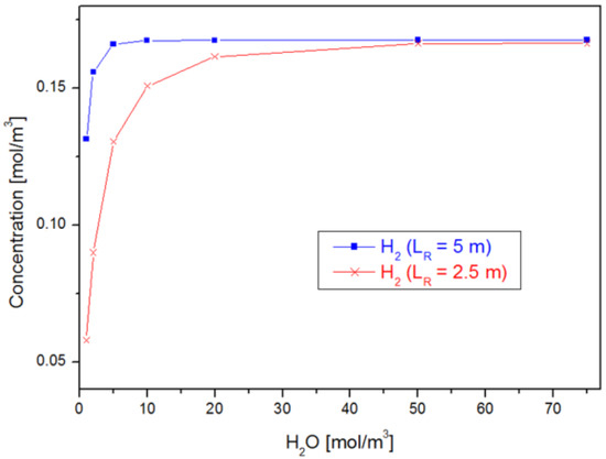
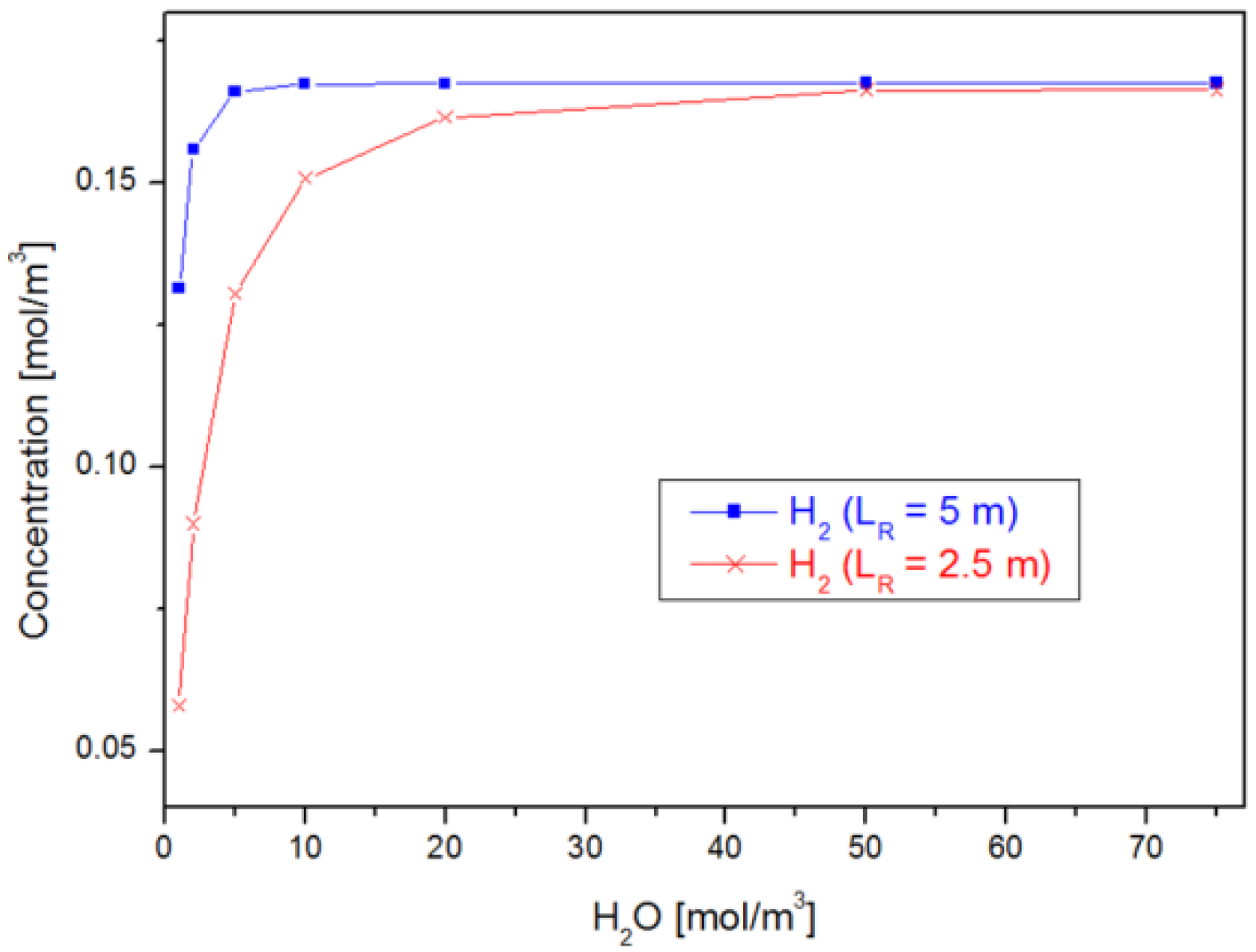
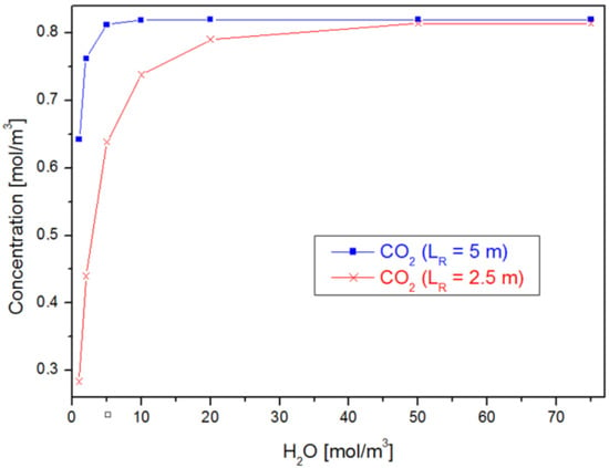
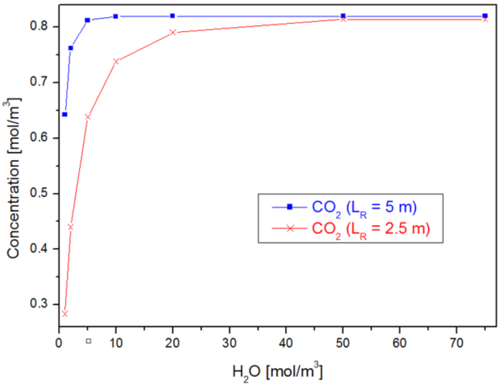
In the first case, the ${\mathrm{H}}_2\mathrm{O}$ was varied by the values 1, 2, 5, 10, 20, 50, and 75 mol/m³ (${\mathrm{H}}_2\mathrm{O}$ inlet), as presented in Figure 5 and Figure 6. Note that, in this case, $L_R$ was varied by 2.5 and 5 m.

Figure 5. Medium concentration values ${\mathrm{H}}_2$ varying ${\mathrm{H}}_2\mathrm{O}$.

Figure 6. Medium concentration values ${\mathrm{CO}}_2$ varying ${\mathrm{H}}_2\mathrm{O}$.

In Figure 5 and Figure 6, some interesting information can be seen: both the production of ${ \mathrm{H}}_2$ and ${\mathrm{CO}}_2$ reached their maximum points close to 50 mol/${\mathrm{m}}^3$ of input ${\mathrm{H}}_2\mathrm{O}$, highlighting that it occurs for $L_R$ equal to both 2.5 and 5 m. Note also that the production of ${\mathrm{CO}}_2$ is prioritized instead of the production of ${\mathrm{H}}_2$ (by 5 times).

4.2. Case 2: Varying the Reactor Geometry ($L_R$)

As in Case 1 the ${\mathrm{H}}_2\mathrm{O}$ inlet concentration equal to 10 mol/${\mathrm{m}}^3$ was found to be a highlight; in this case, the inlet concentration was fixed (${\mathrm{H}}_2\mathrm{O}$ = 10 mol/m³).

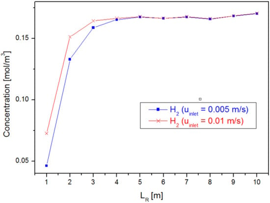
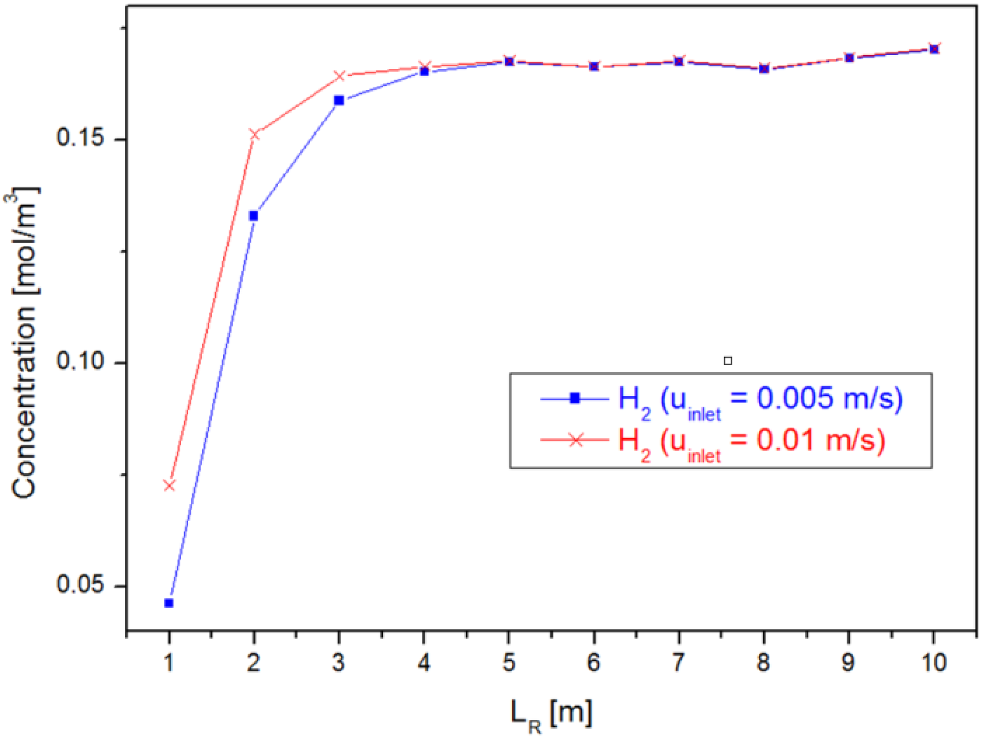
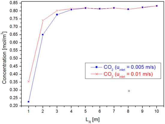
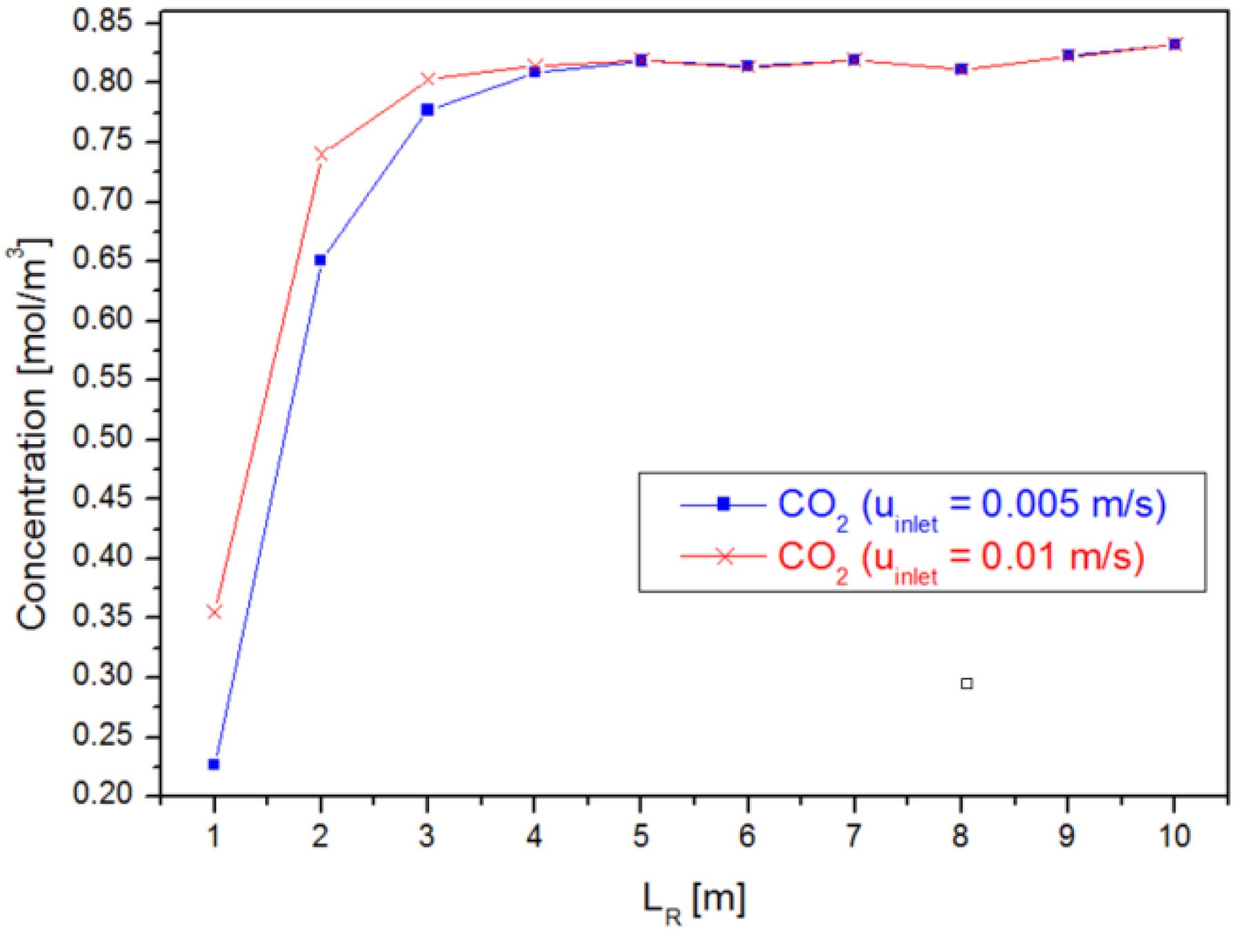
Figure 7 and Figure 8 present the average concentration at the reactor outlet for different reactor sizes for two different inlet ($u_{inlet}$) velocities. As in Case 1, both ${\mathrm{H}}_2$ and ${\mathrm{CO}}_2$ reach a stabilization at the average concentration of the outlet of the reactor around a reactor of length 5 m for two evaluated velocities.

Figure 7. Medium concentration values ${\mathrm{H}}_2$ varying $L_R$.

Figure 8. Medium concentration values ${\mathrm{CO}}_2$ varying $L_R$.

4.3. Case 3: Varying the Inlet Velocity ($u_{inlet}$)

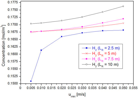
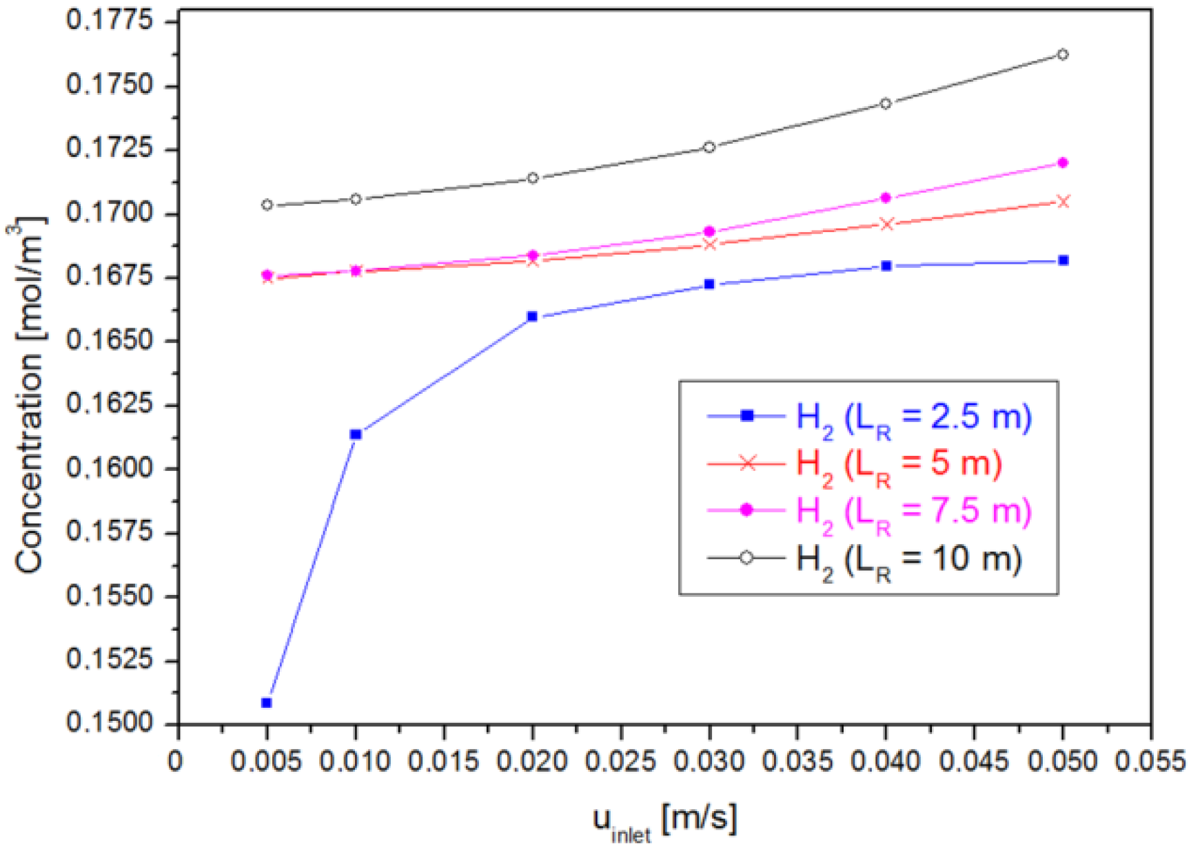
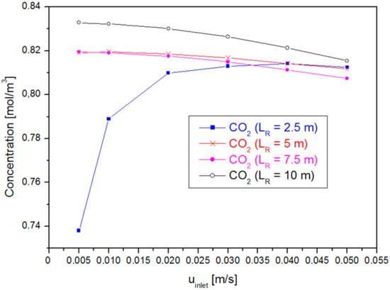
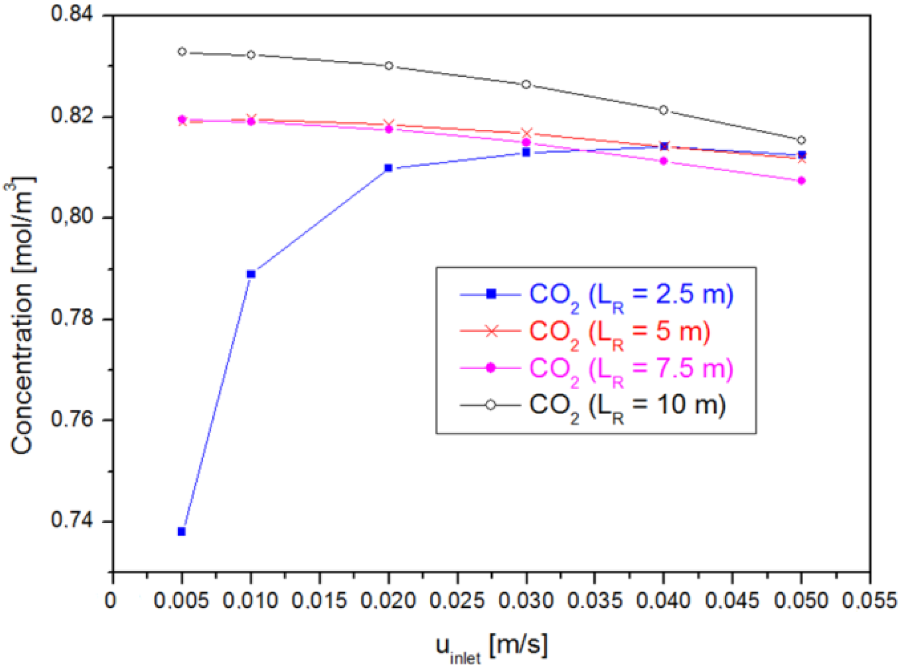
Finally, in this last case, the speed variation will be presented for, again, an ${\mathrm{H}}_2\mathrm{O}$ inlet concentration of 10 mol/${\mathrm{m}}^3$ and for two $L_R$ values, for 5 (highlighted value in Case 2) and 10 m.

As in the first two cases, it is noted that the four $L_R$ variations, together with the $u_{inlet}$ variations, suggest stability of ${\mathrm{H}}_2$ production (Figure 9 and Figure 10), with the caveat that, except in the case of $L_R=2.5 \mathrm{m}$, the other curves are slightly decreasing.

Figure 9. Medium concentration values ${\mathrm{H}}_2$ varying Inlet velocity.

Figure 10. Medium concentration values ${\mathrm{CO}}_2$ varying Inlet speed.

4.4. Optimization

In order to understand how the control variables influence the generation of hydrogen, from the highest production, ${\mathrm{H}}_2=0.175$, found in the condition $L_R=10 \mathrm{m}$, $u_{inlet}$= 0.04 m/s, and ${\mathrm{H}}_2\mathrm{O}=10 \mathrm{mol}/{\mathrm{m}}^3$, for $L_R$ ranging between 1 and 10 m, $u_{inlet}$ between 0.005 and 0.04 m/s, and ${\mathrm{H}}_2\mathrm{O}$ between 1 and 10 $\mathrm{mol}/{\mathrm{m}}^3$, in the dataset analyzed in the previous sections, a new dataset was generated in the simulations, varying p% for more and/or for less the values of the input variables. In this way, the process was repeated, always starting from the highest value found, until obtaining a new set of data with sufficient size to test regression models with three independent variables and their combinations two by two, which, in this case, were four iterations using: p = 0.2, p = 0.1, p = 0.05, and p = 0.05, forming a new dataset with 32 points.

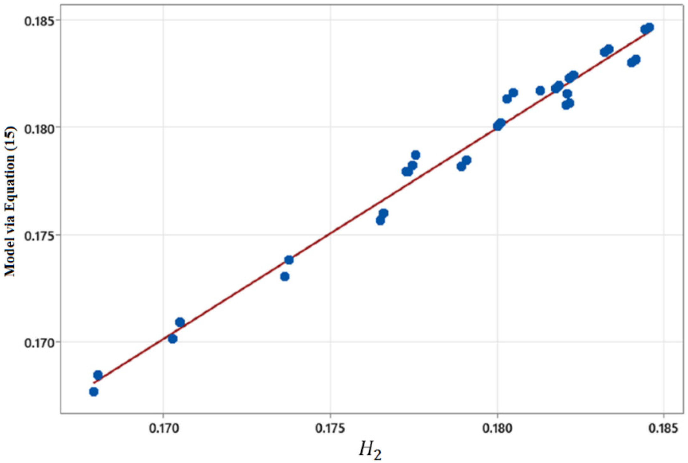
For this new set of data, using the K-fold cross-validation with 10 folds, the best model adjustment was obtained, as shown in Equation (15).

$${\mathrm{H}}_2=0.14429+0.004254L_R-0.151u_{inlet}-0.000196{\mathrm{H}}_2\mathrm{O}-0.000207L_R^2+0.0381L_R{u}_{inlet}$$

(15)

The statistics regarding the quality of adjustment of the model (Equation (15)) are shown in Table 2, in which it is possible to observe that the model fits very well to the simulated data, showing high adjusted R² and cross-validation values, indicating that the model has good generalization capacity with a test for normal residuals (Aderson Darling), p-Value = 0.164.

Table 2. Summary of the quality model fit (Equation (15)).

S	R2	R2 (aj)	R2 (pred)	10-Fold S	10-Fold R2
0.0007019	98.16%	97.81%	97.40%	0.0007624	97.33%

S: sum square; R²: R square; R² (aj): R² adjusted; 10-fold S: sum squared of the validation process 10 folds; 10-fold R²: R² of the 10-fold validation process.

The analysis of the variance of the model (Equation (15)) is shown in Table 3. In this table, it is evident from the analysis of the p-Value and the F-distribution that the variable that most influences the generation of H₂ is $L_R$, followed by $u_{inlet}$. In the region studied, ${\mathrm{H}}_2\mathrm{O}$ has a threshold significance.

Table 3. Analysis of variance for proposed model (Equation (15)).

	GL	SQ (Aj.)	QM (Aj.)	F-Value	p-Value
Regression	5	0.000684	0.000137	277.67	0.000
$L_R$	1	0.000018	0.000018	35.64	0.000
$u_{inlet}$	1	0.000001	0.000001	1.53	0.227
${\mathrm{H}}_2\mathrm{O}$	1	0.000002	0.000002	3.99	0.056
$L_R^2$	1	0.000013	0.000013	25.40	0.000
$L_R\times u_{inlet}$	1	0.000006	0.000006	12.95	0.001
Error	26	0.000013	0.000000
Total	31	0.000697

GL: degrees of freedom; SQ (Aj.): sum squared; QM (Aj.): medium sum squared; F-Value: F distribution value; p-Value: p value.

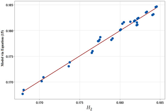
The quality of the adjustment can be observed in Figure 11. It is interesting to observe in this figure that the strategy of prospecting for new data with the objective of obtaining a greater production of ${\mathrm{H}}_2$ appears to be successful because it presents several combinations of $L_R$, $u_{inlet}$, and ${\mathrm{H}}_2\mathrm{O}$, with ${\mathrm{H}}_2$ greater than 0.175 compared with the initial dataset.

Figure 11. Quality of fit of the model (Equation (15)) with respect to simulated ${\mathrm{H}}_2$ production data.

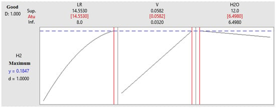
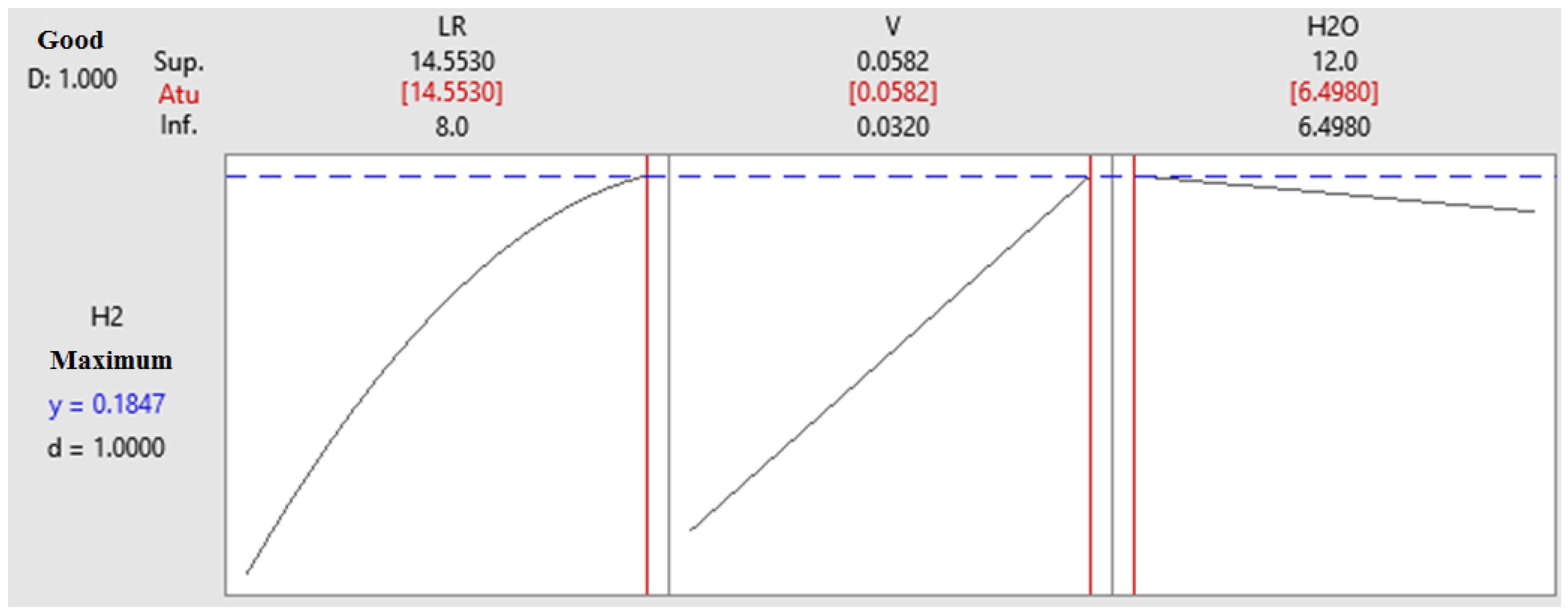
Finally, using Minitab’s optimizer, it is possible to envision a direction toward greater ${\mathrm{H}}_2$ production (Figure 12). In these results, it is evident that a greater production of ${\mathrm{H}}_2$ can be obtained by increasing $L_R$ and $u_{inlet}$ and decreasing ${\mathrm{H}}_2\mathrm{O}$. To assess whether these indications are correct, six more simulations were performed. The results are shown in Table 4, showing a significant increase in ${\mathrm{H}}_2$ production.

Figure 12. Model optimization (Equation (15)) to maximize ${\mathrm{H}}_2$ production.

Table 4. Comparison between simulated values and values predicted by the model.

n	${\mathit{L}}_{\mathit{R}} \left[\mathbf{m}\right]$	${\mathit{u}}_{\mathit{i}\mathit{n}\mathit{l}\mathit{e}\mathit{t}} \left[\frac{{\displaystyle \mathbf{m}}}{{\displaystyle \mathbf{s}}}\right]$	${\mathbf{H}}_2\mathbf{O} \left[\frac{\mathbf{m}\mathbf{o}\mathbf{l}}{{\mathbf{m}}^3}\right]$	${\mathbf{H}}_2 \left[\frac{\mathbf{m}\mathbf{o}\mathbf{l}}{{\mathbf{m}}^3}\right]$	Prediction	LIMP	LISP
1	15	0.065	6	0.190	0.188	0.1854	0.1902
2	15.5	0.07	5.5	0.193	0.190	0.1875	0.1932
3	16	0.08	5	0.201	0.195	0.1912	0.1992
4	18	0.09	4	0.207	0.201	0.1947	0.2080
5	19	0.15	3.5	0.266	0.236	0.2158	0.2559
6	20	0.2	3	0.336	0.268	0.2337	0.3032

LIMP: bottom limit of prediction; LISP: upper limit of prediction.

In addition, the predictions of the proposed model, even under the extrapolation condition, are close to the simulated values, and several points are within the prediction confidence interval (99%). It is interesting to note that in point 6 there is a large discrepancy between the value of the simulation and the proposed model.

This may be an indication of the use of the proposed model in an excessively extrapolated way or also that there was a change in the flow regime because the data were simulated in the laminar flow condition. In fact, subsequent attempts to simulate the production of hydrogen with higher velocities were not possible due to the numerical divergence presented by COMSOL, possibly due to entering a turbulent flow regime.

5. Conclusions

It can be concluded from this study that, considering only three parameters, it is possible to simulate the production of ${\mathrm{H}}_2$ and ${\mathrm{CO}}_2$, in order to identify the optimized equation for these defined boundary conditions.

The great influence of the geometry on the concentration of the products is noticed, whereas after $L_R$ greater than 5, the variation of ${\mathrm{H}}_2\mathrm{O}$ becomes negligible and the production of ${\mathrm{H}}_2$ is prioritized instead of ${\mathrm{CO}}_2$. The identified optimization equation has a high accuracy rate, corroborating with the idealization of the project and opening opportunities for the development of other studies considering the different conditions of the proposals in this paper.

Finally, it is concluded that this study, in addition to its many possible variations, contributes to the theme of sustainability, which has been growing on the world stage, and to the development of new technologies for the benefit of society, in addition to searching for new feasible alternatives for the more efficient production of energy.

References

- Teixeira, C.A.N.; Mendes, A.P.d.A.; Costa, R.C.d.; Rocio, M.A.R.; Prates, H.F. Natural Gas—A Key Fuel for a Low-Carbon Economy; Banco Nacional de Desenvolvimento Econômico e Social: Rio de Janeiro, Brazil, 2021; Volume 27, pp. 131–175. [Google Scholar]
- Santos, E.M.dos; Fagá, M.T.W.; Barufi, C.B.; Poulallion, P.L. Gás Natural: A construção de uma nova civilização. Estud. Avançados 2007, 21, 67–90. (In Portuguese) [Google Scholar] [CrossRef] [Scilit]
- Prates, C.P.T.; Pierobon, E.C.; Costa, R.C.d.; Figueiredo, V.S.d. Evolução da Oferta e da Demanda de Gás Natural no Brasil; Banco Nacional de Desenvolvimento Econômico e Social: Rio de Janeiro, Brazil, 2006; pp. 35–68. (In Portuguese) [Google Scholar]
- Lacerda, A.; Leroux, T.; Morata, T. Efeitos Ototóxicos da Exposição ao Monóxido de Carbono: Uma Revisão. Pró-Fono Rev. Atualização Cient. 2005, 17, 403–412. [Google Scholar] [CrossRef] [Scilit] [PubMed]
- Oliveira, N.M.B. Fundamentos de Cinética e Introdução ao Cálculo de Reatores; Editora e Distribuidora Educacional S.A.: Londrina, Brazil, 2017. (In Portuguese) [Google Scholar]
- Chang, R. Química Geral—Conceitos Essenciais; Bookman: Porto Alegre, Brazil, 2007; p. 778. (In Portuguese) [Google Scholar]
- Fernandes, R.F. Catalisador. Rev. Ciênc. Elem. 2015, 3, 36. [Google Scholar] [CrossRef] [Scilit]
- Atkins, P.; Jones, L. Princípios de Química: Questionando a Vida Moderna e o Meio Ambiente, 5th ed.; Bookman: Porto Alegre, Brazil, 2011; p. 1048. [Google Scholar]
- Cremasco, M.A. Difusão Mássica; Editora Blucher: São Paulo, Brazil, 2019; p. 285. [Google Scholar]
- Xu, J.; Froment, G.F. Methane Steam Reforming, Methanation and Water-Gas Shift: 1. Intrinsic Kinetics. AIChE J. 1989, 35, 88–96. [Google Scholar] [CrossRef] [Scilit]
- COMSOL. Available online: https://doc.comsol.com/5.6/doc/com.comsol.help.cfd/cfd_ug_fluidflow_porous.10.37.html (accessed on 23 November 2022).
- COMSOL. Available online: https://doc.comsol.com/5.6/doc/com.comsol.help.chem/chem_ug_chemsptrans.08.050.html (accessed on 23 November 2022).
Disclaimer/Publisher’s Note: The statements, opinions and data contained in all publications are solely those of the individual author(s) and contributor(s) and not of MDPI and/or the editor(s). MDPI and/or the editor(s) disclaim responsibility for any injury to people or property resulting from any ideas, methods, instructions or products referred to in the content. |
© 2023 by the authors. Licensee MDPI, Basel, Switzerland. This article is an open access article distributed under the terms and conditions of the Creative Commons Attribution (CC BY) license (https://creativecommons.org/licenses/by/4.0/).