A Variable-Fidelity Multi-Objective Evolutionary Method for Polygonal Pin Fin Heat Sink Design

Abstract

For the multi-objective design of heat sinks, several evolutionary algorithms usually require many iterations to converge, which is computationally expensive. Variable-fidelity multi-objective (VFO) methods were suggested to improve the efficiency of evolutionary algorithms. However, multi-objective problems are seldom optimized using VFO. Therefore, a variable-fidelity evolutionary method (VFMEM) was suggested. Similar to other variable-fidelity algorithms, VFMEM solves a high-fidelity model using a low-fidelity model. Compared with other algorithms, the distinctive characteristic of VFMEM is its application in multi-objective optimization. First, the suggested method uses a low-fidelity model to locate the region where the global optimal solution might be found. Sequentially, both high- and low-fidelity models can be integrated to find the real global optimal solution. Circulation distance elimination (CDE) was suggested to uniformly obtain the PF. To evaluate the feasibility of VFMEM, two classical benchmark functions were tested. Compared with the widely used multi-objective particle swarm optimization (MOPSO), the efficiency of VFMEM was significantly improved and the Pareto frontier (PFs) could also be obtained. To evaluate the algorithm’s feasibility, a polygonal pin fin heat sink (PFHS) design was carried out using VFMEM. Compared with the initial design, the results showed that the mass, base temperature, and temperature difference of the designed optimum heat sink were decreased 5.5%, 18.5%, and 62.0%, respectively. More importantly, if the design was completed directly by MOPSO, the computational cost of the entire optimization procedure would be significantly increased.

1. Introduction

Efficiently cooling the heat of electronic systems and uniformly distributing the heat is an important issue for thermal management. To enhance the heat transfer ability, many kinds of optimization methods have been applied to the design of heat sinks. Husain and Kim [1] performed shape optimization of a microchannel heat sink, and obtained pareto-optimal solutions using a fast and elitist non-dominated sorting genetic algorithm (NSGA-II). Srisomporn and Bureerat [2] demonstrated the use of the strength pareto evolutionary algorithm (SPEA), with and without the combination of RSM, for a multi-objective design of plate-fin heat sink geometry. The purpose of this study is to minimize the heat sink junction temperature and fan pumping power. Bureerat and Srisomporn [3] used a multi-objective evolutionary algorithm (MOEA), namely population-based incremental learning (PBIL), to minimize the junction temperature and fan pumping power while meeting predefined constraints. Kanyakam and Bureerat [4] obtained the optimal geometric parameters of the PFHS with proposals of the minimum junction temperature and fan power. Lampio and Karvinen [5] used a multi-objective version of the particle swarm optimization (PSO) method to optimize the heat sink performance in forced and natural convection cases. For both cases, mass was minimized. The other criteria included maximizing the temperature for the forced convection case and heat sink outer volume for the natural convection case. Huang and Wang [6] used global sensitivity analysis to analyze and optimize the cooling method. Pourfattah and Sabzpooshani [7] combined the genetic algorithm (GA) and RSM to design the cooling system.

According to above mentioned applications, most cases can be optimized using evolutionary algorithms (EAs), such as GA (genetic algorithm), PSO, SPEA, and PBIL, because these methods can theoretically find the global optimal solution. However, these evolutionary algorithms usually require a large number of evaluations to converge. Obviously, if the heat sink design is optimized directly using evolutionary algorithms, especially for expensive evaluation problems, the computational cost is not feasible in practice. Thus, to improve the efficiency of optimization, VFMEM is suggested. Compared with related methods, both high- and low-fidelity models are constructed. The low-fidelity model is employed to roughly locate the global optimization region, thus the computational cost can be significantly reduced. In contrast, the high-fidelity model is introduced to exploit the global optimal region, enabling the accurate solution to be achieved. Compared with evolutionary algorithms, the suggested method can efficiently achieve global optimization.

In this study, the design of a heat sink with polygonal pin fins is a natural convection case with nine design variables. As a commonly used heat transfer enhancement device, the PFHS is widely used in the heat dissipation of electronic components. Different shapes of PFHSs affect the heat transfer performance of the heat sink. To date, numerous studies have been dedicated to the optimization of heat sinks with various fin geometries, such as rectangular, diamond, square, pentagonal, or cylindrical geometries. Ramphueiphad and Bureerat [8] and Vanapalli and Brake [9] studied six different pin fins with the same cross section. Matsumoto et al. [10] experimentally and numerically studied five types of PFHS under natural convection and analyzed the influences of the size, height, and number of fins on the thermal performance. Zhao et al. [11] numerically studied flow and heat transfer characteristics of micro square PFHS and obtained optimal geometric parameters. Although this problem has been widely investigated, few studies have used an optimization method for PFHS structural design. Therefore, the introduction of a multi-objective design for PFHS should further improve heat transfer performance.

The rest of paper is organized as follows. Section 2 describes some basic concepts related VFO and EA. Section 3 presents the details of the suggested method. Two cases are carried out to evaluate the performance of the suggested method in Section 4. In Section 5, a PFHS structural design is successfully solved by VFMEM. Finally, the conclusion is given.

2. Basic Theories and Literature Review for VFO

2.1. Variable Fidelity Optimization

VFO can be described as an optimization process that integrates a low-fidelity model (LFM) and a high-fidelity Model (HFM). For most problems, the fidelity suggests high accuracy, stable solution, such as a fine finite element model. The optimization direction should be often corrected and modified in an iterative process [12]. The LFM and HFM are employed to reduce the computation cost and improve the accuracy of the LFM. The description of VFO and related other important methods are given below.

2.1.1. Framework of VFO

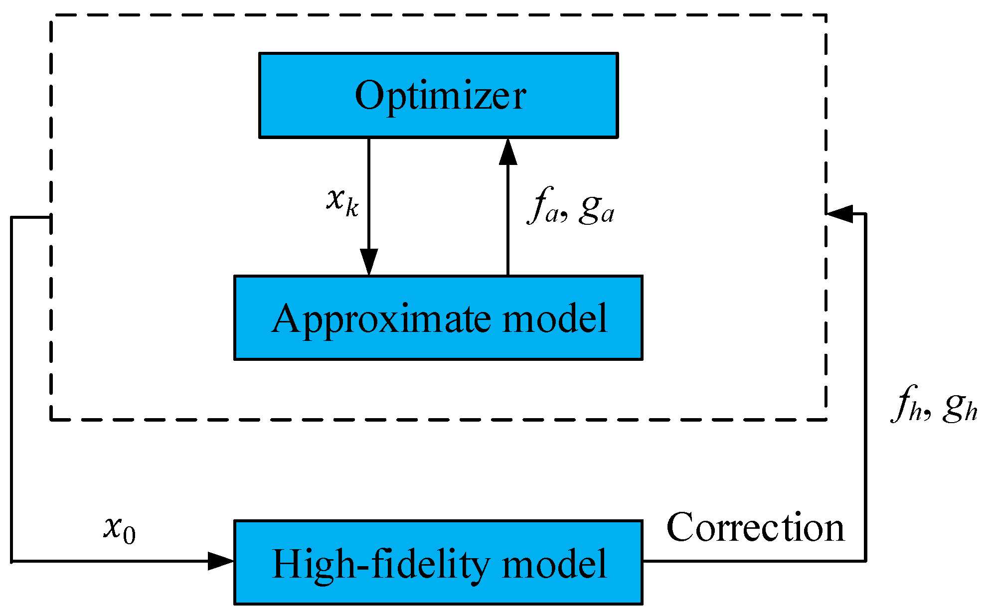
VFO schemes have been developed in various forms [13]. Scaling based frameworks for VFO were first developed by Chang et al. [14]. They used a multiplicative scaling function to update the responses of LFMs to match those of HFMs. Alexandrov and Lewis [15] presented a first-order model management optimization methodology for solving high-fidelity optimization problems with minimal expense in HFM and derivative evaluation. Gano et al. [16] proposed a hybrid approach for scaling management, in which the hybrid scaling method was combined between multiplicative and additive scaling methods by the weighting factor. Figure 1 shows such a simple description of the variable-fidelity framework [12].

In Figure 1, $x$ denotes design variable; $f_a$ and g_a denote the values of approximate model (low-fidelity) and corresponding sensitivity, respectively. $f_h$ and g_h denote values of HFM and corresponding sensitivity. The initial responses of design of experiments (DoE) are obtained by LFM at cheap computational cost. Then, it should be validated by information obtained from the HFM. Sequentially, the optimization procedure is performed by the LFM. Finally, the LFM is calibrated with the HFM and optimization is continued using the LFM until the convergence criteria are satisfied.

2.1.2. Space Mapping

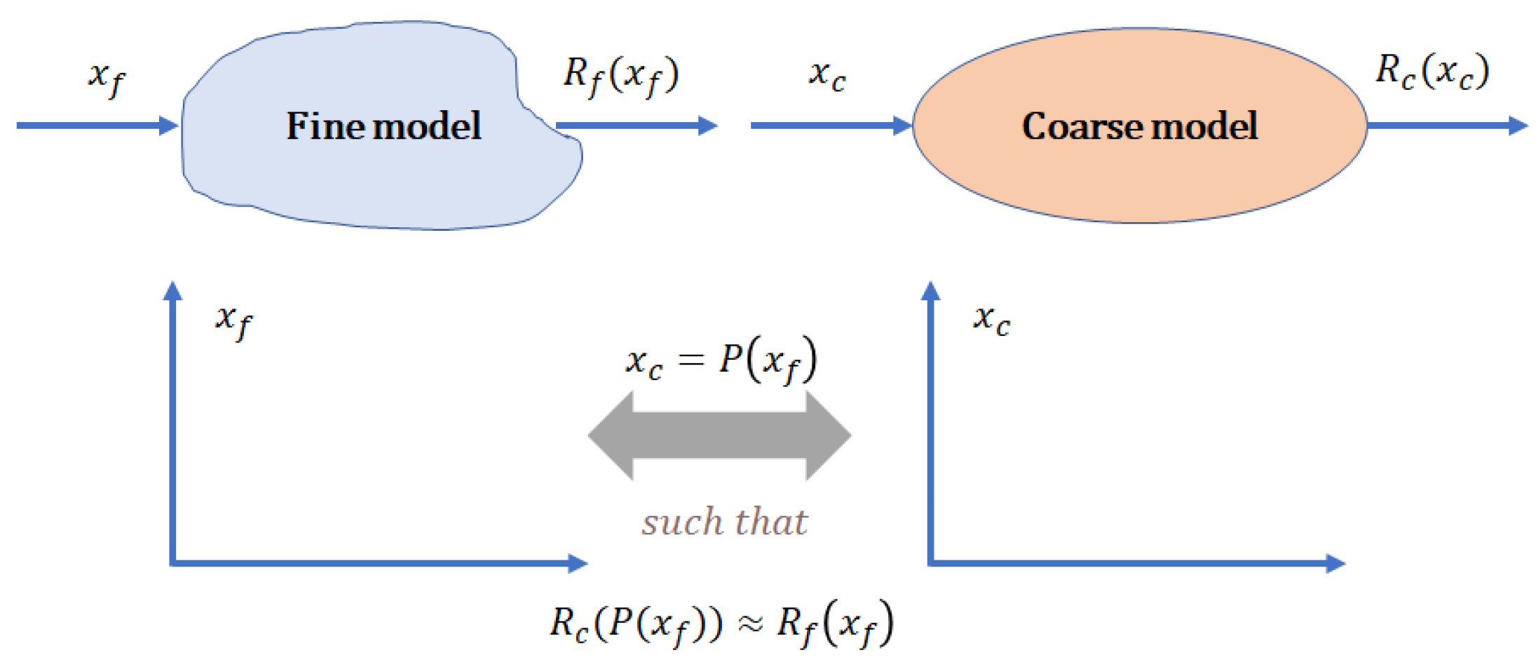
Space mapping (SM) is another important branch of VFO that also uses a fine model (HFM) with a coarse model (LFM) to reduce the computational cost of evaluation based on the HFM. The SM algorithm first proposed by Bandler et al. [17] was originally applied to circuit optimization and has been applied in related fields [18]. The essential idea of the SM is to construct the projection between coarse and fine spaces. Parameter extraction (PE) is a crucial procedure for SM. The framework of SM can be described as Figure 2 [19].

In Figure 2, $x_c$ and $x_f$ are design parameters of the coarse and fine models, respectively, and $R_c\left(x_c\right)$ and $R_f\left(x_f\right)$ denote corresponding model responses. As illustrated in Figure 2, the purpose of SM is to find an appropriate mapping p from the fine model parameter space $x_f$ to the coarse model parameter space $x_c$, as given by:

$$x_c=P\left(x_f\right)$$

(1)

such that

$$R_c(P(x_f))\approx R_f\left(x_f\right)$$

(2)

Once mapping is obtained, the coarse model can be used for fast and accurate evaluations. Compared with direct optimization methods without coarse models, the efficiency can be significantly improved with SM. With the development of the SM algorithm, several approaches have utilized SM algorithms in engineering modeling, such as by Bandler and Ismail [19] and Echeverria and Hemker [20]. However, SM has difficulty handling increasing nonlinearity in physical models, posing a challenge for complicated practical problems. As tested by Wang et al. [21], highly nonlinear problems are difficult for SM to handle due to the PE procedure. Moreover, if the response of a coarse model is widely different from that of a fine model, the convergence of SM cannot be guaranteed. To control the coarse model’s accuracy in a limited range and guarantee the convergence of SM, reanalysis-based SM (RBSM) was proposed by Wang et al. [22]. They used the reanalysis method to substitute the coarse model to analyze finite element (FE) models. However, some problems with SM remain. The SM is seldom considered for multi-objective optimization. To overcome this bottleneck, VFMEM is suggested for multi-objective optimization.

2.2. PSO

2.2.1. Standard PSO

PSO is a random, population-based evolutionary algorithm proposed by Eberhart and Kennedy [23]. PSO is inspired by the social behavior of organisms such as bird flocking and fish schooling. The search starts with a population of search points called particles. The velocity and position of the kth particle are represented as ${\overrightarrow{v}}_i=\left[v_{i1},v_{i2},\dots ,v_{in}\right]$ and ${\overrightarrow{x}}_i=\left[x_{i1},x_{i2},\dots ,x_{in}\right]$. The velocity and position of the kth particle are updated as follows:

$${\overrightarrow{v}}_i^{t+1}=\omega {\overrightarrow{v}}_i^t+c_1{r}_1\left({\overrightarrow{p}}_i^t-{\overrightarrow{x}}_i^t\right)+c_2{r}_2\left({\overrightarrow{p}}_g^t-{\overrightarrow{x}}_i^t\right)$$

(3)

$${\overrightarrow{x}}_i^{t+1}={\overrightarrow{x}}_i^t+{\overrightarrow{v}}_i^{t+1}$$

(4)

where ${\overrightarrow{v}}_i^t$ and ${\overrightarrow{x}}_i^t$ are the velocity and position of the ith particle at the tth iteration, respectively; $c_1$ and $c_2$ are the cognitive and social coefficients; $r_1$ and $r_2$ are elements from two uniform random sequences in the range of [0, 1]; ${\overrightarrow{p}}_i^t$ is the best previous position of the ith particle, ${\overrightarrow{p}}_g^t$ is the best position among the whole swarm, and $\omega$ is the inertia weight, which is used to balance the local and global search [24]. Higher inertia constitutes a global search by putting more weight on the previous experience and a lower inertia facilitates the local search.

2.2.2. Multi-Objective PSO (MOPSO)

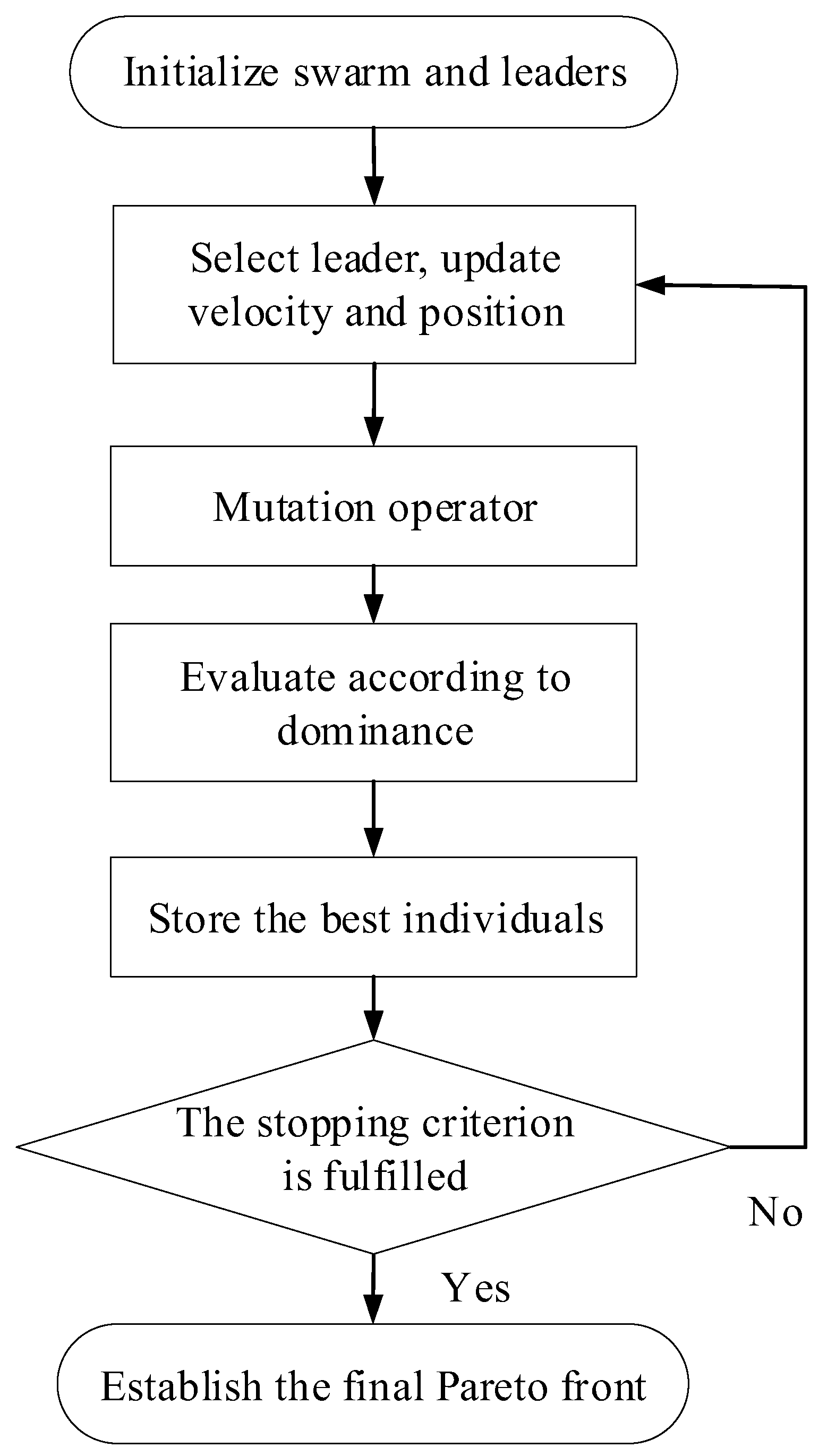
To apply the PSO strategy to solve multi-objective optimization problems, many approaches have been embedded into PSO [25,26,27,28,29]. In the PSO, multi-objective optimization algorithms use the concept of Pareto front, and the best non-dominated positions (leaders) are used to guide particles [30]. To maintain the Pareto optimal solutions identified, an additional set, called the external register, is used to store the non-dominated solutions discovered during the search. A new solution is included in the register if it is not dominated by all of its members. If some members are dominated by the new solution, it is usually removed from the registry. Most of the existing MOPSO algorithms apply some sort of mutation operator [30]. Figure 3 shows the flow chart of a MOPSO algorithm.

Although some significant improvements have been achieved in MOPSO, the MOPSO algorithm still requires many iterations to converge. For most expensive evaluation problems, the computational cost remains expensive and difficult to implement. Therefore, we hope to integrate VFO and MOPSO to improve the efficiency of multi-objective optimization in practice with guaranteed accuracy practically.

3. Variable-Fidelity Multi-Objective Evolutionary Method (VFMEM)

VFMEM is based on the integration of VFO and MOPSO algorithms. In VFMEM, the LFM is for global searching and HFM is for local searching. As mentioned before, circulation distance elimination (CDE) and parameter transfer (PT) strategies are integrated so that VFMEM can use LFMs and HFMs according to the accuracy criterion. The CDE strategy is to uniformly select part of the optimal solutions from the LFM’s Pareto set in order to reduce the number of calculations of the HFM. The PT strategy is used to transfer the parameters of the selected optimal solutions of the LFM to the HFM so that the HFM can perform the local search more easily and accurately.

3.1. CDE

Usually, some particles of the Pareto frontier (PF) are locally concentrated after optimization of the LFM. If all of them are transferred by the PT, the amount of evaluation of the HFM will be greatly increased. Therefore, the CDE strategy is used to select part of the uniformly distributed particles. It is well known that the search direction of optimization is influenced by the accuracy of the physical model. If the LFM is too coarse, the direction of optimization may be wrong. Therefore, the two models are required to be similar. It is helpful for the HFM to obtain Pareto solutions with uniform distribution at the beginning by transferring the parameters of the uniformly distributed particles.

Before the selection of solutions from the LFM’s PF, the LFM’s objectives are all normalized to a range [0, 1]

$$f_{sk}=\frac{f_k-f_{k,min}}{f_{k,max}-f_{k,min}}$$

(5)

where $f_k$ is the function value of the kth objective, $f_{k,min}$ and $f_{k,max}$ are respectively the minimum and maximum function values of the kth objective, and $f_{sk}$ denotes the scaled kth objective function values.

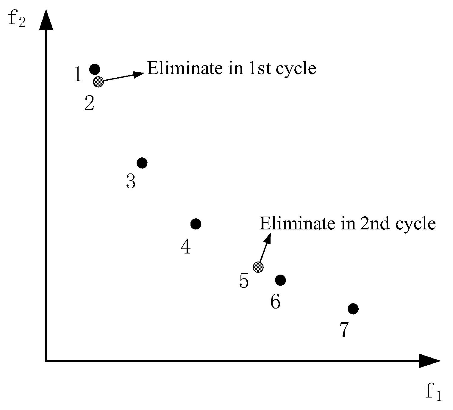
It is well known that the calculation of the Euclidean distance in design space between any two particles reflects their degrees of closeness. Figure 4 shows the procedure of selecting PF. As shown in Figure 4, the minimum Euclidean distance is between particles 1 and 2 of the obtained PF. First, the procedure should randomly eliminate one of the particles, and assume the removed particle is the second in the pair. Then, the Euclidean distance of any two particles in the rest should be calculated and sorted. In the rest of the particles, the minimum Euclidean distance is between particles 5 and 6. Similarly, one of the two particles should be randomly removed, and assume the removed particle is fifth one, and so on. The final particles are those that need to be preserved. Figure 5 shows the pseudocode of the CDE. After completion of the CDE procedure, the information of the selected optimal solutions of LFM will be transferred to HFM through the PT strategy.

3.2. PT

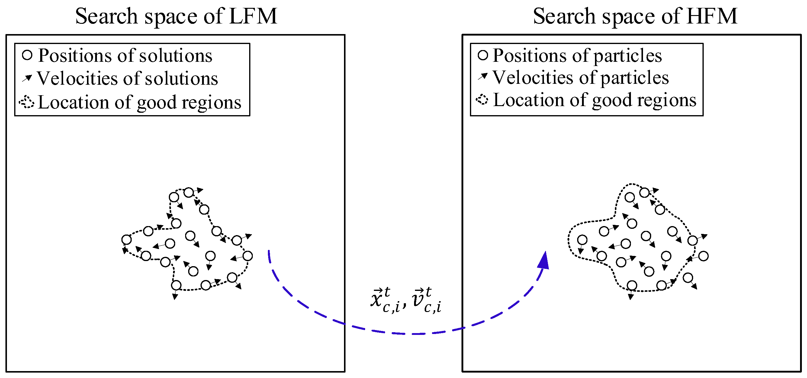
After optimization of the LFM, the particles usually search in the local regions. It is a critical issue to determine the searching direction. The search direction based on the HFM should guarantee the convergence of the entire optimization procedure. The parameters that need to be transferred are the velocities and positions of the LFM. As shown in Figure 6, the velocities ${\overrightarrow{v}}_{c,i}^t$ and positions ${\overrightarrow{x}}_{c,i}^t$ of the LFM’s solutions selected by the CDE are used as the velocities ${\overrightarrow{v}}_{f,i}^0$ and positions ${\overrightarrow{x}}_{f,i}^0$ of the HFM’s initial population.

$${\overrightarrow{v}}_{f,i}^0={\overrightarrow{v}}_{c,i}^t$$

(6)

$${\overrightarrow{x}}_{f,i}^0={\overrightarrow{x}}_{c,i}^t$$

(7)

Considering that the two models are required to be similar, some of the particles might be transferred in the good regions when the transformation is complete. This might efficiently improve the convergence ratio. However, if the two models are widely different, it might lead to the wrong direction in the design space. Therefore, it is important to guarantee the accuracy of the LFM. Generally, the trend of the LFM should be in accordance. The criteria for this issue are presented in the following sections.

3.3. VFMEM

In this section, CDE and PT strategies are integrated in MOPSO. MOPSO is used to obtain the Pareto optimal solutions of the LFM and then the HFM. Theoretically, any multi-objective optimization can be used. MOPSO is engaged to reduce the control parameters. The CDE strategy is applied to uniformly select particles from the LFM’s Pareto-optimal set, and the PT strategy is used to transfer the parameters of the selected optimal particles of the LFM to the HFM.

The process of VFMEM is presented as follows:

Step 1 The Pareto-optimal set $X_c^{*}$ is obtained by MOPSO based on the LFM.

Step 2n solutions are selected from $X_c^{*}$ by using the CDE;

Step 3 The velocities and positions of the chosen optimal particles, which are defined in Equations (6) and (7), are used as the velocities and positions of the HFM’s particle by the PT strategy. Since there should be some differences between two models, the value of weight $\omega$ should be initialized.

Step 4 Initialize the HFM, and the velocity and position of the ith particle of HFM are updated as follows:

$${\overrightarrow{v}}_{f,i}^{t+1}=\omega {\overrightarrow{v}}_{f,i}^0+c_1{r}_1\left({\overrightarrow{p}}_i^t-{\overrightarrow{x}}_{f,i}^0\right)+c_2{r}_2\left({\overrightarrow{p}}_g^t-{\overrightarrow{x}}_{f,i}^0\right)$$

(8)

$${\overrightarrow{x}}_{f,i}^{t+1}={\overrightarrow{x}}_{f,i}^0+{\overrightarrow{v}}_{f,i}^{t+1}$$

(9)

Step 5 Obtain the Pareto-optimal set of the HFM in the initialization and compare the responses of two models’ objectives. The similarity of the two models is verified by calculating their average relative error in the objectives

$$E_{ave}=\frac{{\sum }_{j=1}^k{\sum }_{i=1}^n\left|\frac{y_h^{i,j}-y_l^{i,j}}{y_h^{i,j}}\right|}{nk}$$

(10)

where n is the number of solutions selected by the CDE, k is the number of objectives, $y_h^{i,j}$ and $y_l^{i,j}$ are the objective values of the HFM and LFM, respectively. The smaller the $E_{ave}$ value, the more similar the two models. The value $E_{ave}=0$ indicates that the two models are the same. In this study, if $E_{ave}>20\%$ indicated a great difference between the two models. Then procedure reconstructs an LFM with higher accuracy and goes to step 1 (If the LFM is a FE model with coarse grid, the accuracy of the LFM can be changed by using a finer grid. If it is a data fitting model such as the classical response surface model (RSM), spline, or kriging model, the accuracy can be changed by increasing the data of the HFM’s initialization). If not, the procedure goes to step 6.

Step 6 The HFM is optimized using MOPSO. In the LFM-based optimization procedure, the value of the error between the two iterative steps named IE (iteration error) usually decreases gradually. The value of IE usually maintains a relatively stable value in the final optimization. Since the two models are similar, refer to the LFM. If the IE value of the HFM is smaller than the given value, the optimization is terminated and the HFM’s Pareto-optimal set $X_f^{*}$ is obtained.

The procedure of VFMEM is shown in Figure 7. In the suggested procedure, if two models are similar, the particles of the HFM can easily to find the locations of good regions in the search space and obtain the Pareto optimal solutions.

4. Performance Assessment with Benchmarks

4.1. Performance Indicators

In the multi-objective problem, the quality of the Pareto-optimal set involves two aspects: the closeness of PF to the true PF and the extent of the PF. In this section, four performance indicators, generational distance (GD) [31], spacing (SP) [32], iterative error (IE), and number (N) are employed to assess the performance.

(1) Generational distance

A criterion that estimates the distance from the elements in the set of non-dominated vectors found so far to those in the Pareto-optimal set. It is defined as:

$$GD=\frac{\sqrt{{\sum }_{i=1}^n{d}_i^2}}{n}$$

(11)

where n is the number of vectors in the set of non-dominated solutions found so far and $d_i$ is the Euclidean distance between each of these and the nearest member of the Pareto-optimal set. $GD=0$ indicates that all the elements generated are in the Pareto-optimal set.

(2) Spacing

A criterion that determines how well the solutions in the current PF are distributed. It is defined as:

$$SP=\sqrt{\frac{1}{n-1}{\displaystyle \sum }_{i=1}^n{\left(\overline{d}-d_i\right)}^2}$$

(12)

$$d_i=\underset{j}{\min }({\sum }_{k=1}^m\left|f_k^i\left(x\right)-f_k^j\left(x\right)\right|)$$

(13)

$$i,j=1,\dots ,n \mathrm{and} j\ne i$$

where n is the number of non-dominated vectors found so far and $\overline{d}$ is the mean of all $d_i$. A value of zero for this metric indicates that all members of the Pareto front currently available are equidistantly spaced. A smaller value represents better diversity of the current Pareto front.

(3) Iterative error

Similar to $GD$, IE estimates the distance of non-dominated vectors between two iteration steps. It is given by:

$$IE=\frac{\sqrt{{\sum }_{i=1}^n{d}_i^2}}{n}$$

(14)

where n is the number of non-dominated solutions in the current iteration, $d_i$ is the Euclidean distance between each of these and the nearest member of the non-dominated solutions in the last iteration. When the method searches in the global region, the value of $IE$ will change considerably because of the large change in the target value, but when the method searches in the local region, $IE$ will be a small value. A smaller value represents a greater possibility that the method is searching in the local region.

(4) Number

The maximal number of elements of the Pareto-optimal set is required.

4.2. Benchmarks

To verify the performance of VFMEM, two test functions ZDT3 [33] and UF8 [34] are studied. The comparison carried out in this study was only based on MOPSO and VFMEM. In our opinion, other multi-objective functions can be theoretically used in the suggested framework. Therefore, such comparisons can evaluate the performance of VFMEM.

4.2.1. Case I: ZDT3 Function

ZDT3 function has a discontinuous Pareto front that consists of five slightly convex parts, and is formulated as follows:

$$\{\begin{array}{c}{f}_1\left(x\right)=x_1\hfill \\ f_2\left(x\right)=g\left(x\right)\left[1-\sqrt{x_1/g\left(x\right)}-\frac{x_1}{g\left(x\right)}\sin \left(10\pi x_1\right)\right]\hfill \\ g\left(x\right)=1+9({\displaystyle \sum _{i=2}^n}{x}_i)/\left(n-1\right)\hfill \end{array} \left(x\in \left[0, 1\right]\right)$$

(15)

The approximation function is constructed according to ZDT3:

$$\{\begin{array}{c}{f}_1\left(x\right)=x_1\hfill \\ f_2\left(x\right)=1.1g\left(x\right)\left[1-\sqrt{1.1x_1/g\left(x\right)}-\frac{1.1x_1}{g\left(x\right)}\sin \left(9\pi x_1\right)\right]\hfill \\ g\left(x\right)=5+9({\displaystyle \sum _{i=2}^n}{x}_i)/(n-1)\hfill \end{array} \left(x\in \left[0, 1\right]\right)$$

(16)

Equation (15) is used as the HFM and Equation (16) is used for the LFM. The number of design variables was set to 30, and the maximum number of iterations was set to 200 for optimizing the LFM and 5 for optimizing the HFM. The size of the repository was 100 for both models. There were 50 particles for the LFM. The number selected through the CED was 30. Let $\omega =$0.9, $c_1=$1.0, $c_2=$ 2.0. A comparison of the results is shown in Figure 8.

In order to compare the performance of the presented method, a direct optimization of the HFM was implemented using MOPSO. The number of design variables was set to 30. The population of particles was set to 30. According to Figure 8, it can be seen that although there was a greater difference between the two models, the method obtained the Pareto optimal solutions of the HFM with fewer calculations.

Table 1. GD, SP, N, and IE of Pareto optimal solutions metrics and optimization history for ZDT3 function using VFMEM.

Iter	GD	SP	N	IE
1	0.0033	0.0721	22	0.0266
2	0.0030	0.0937	30	0.0070
3	0.0024	0.0225	43	0.0054
4	0.0019	0.0118	49	0.0047
5	8.918 × 10−4	0.0076	54	0.0030

and

Table 2. GD, SP, and N of Pareto optimal solutions metrics for ZDT3 function by direct optimization.

Iter	GD	SP	N
100	0.0248	0.0076	31

show the GD, SP, N, and IE values of the Pareto optimal solutions metrics and optimization history for the ZDT3 function.

4.2.2. Case II: UF8 Function

The UF8 function has three objectives; its true Pareto front is $f_1^2+f_2^2+f_3^3=1, 0\le f_1, f_2, f_3\le 1$, and it is formulated as follows:

$$\{\begin{array}{c}{f}_1=\cos \left(0.5x_1\pi \right)\cos \left(0.5x_2\pi \right)+\frac{2}{\left|J_1\right|} {\displaystyle \sum _{j\in J_1}}{\left(x_j-2x_2\sin \left(2\pi x_1+\frac{j\pi }{n}\right)\right)}^2\hfill \\ f_2=\cos \left(0.5x_1\pi \right)\cos \left(0.5x_2\pi \right)+\frac{2}{\left|J_2\right|} {\displaystyle \sum _{j\in J_2}}{\left(x_j-2x_2\sin \left(2\pi x_1+\frac{j\pi }{n}\right)\right)}^2\hfill \\ f_3= \sin \left(0.5x_1\pi \right) +\frac{2}{\left|J_3\right|} {\displaystyle \sum _{j\in J_3}}{\left(x_j-2x_2\sin \left(2\pi x_1+\frac{j\pi }{n}\right)\right)}^2\hfill \end{array}$$

(17)

where

$$J_1=\left\{j|3\le j\le n,\mathrm{and}j-1\mathrm{is}\mathrm{a}\mathrm{multiplication}\mathrm{of}3\right\},$$

$$J_2=\left\{j|3\le j\le n,\mathrm{and}j-2\mathrm{is}\mathrm{a}\mathrm{multiplication}\mathrm{of} 3\right\},$$

$$J_3=\left\{j|3\le j\le n,\mathrm{and}j\mathrm{is}\mathrm{a}\mathrm{multiplication}\mathrm{of} 3\right\}.$$

The approximation function of UF8 is:

$$\{\begin{array}{c}{f}_1=2\cos \left(0.5x_1\pi \right)\cos \left(0.5x_2\pi \right)+\frac{5}{\left|J_1\right|} {\displaystyle \sum _{j\in J_1}}{\left(x_j-x_2\sin \left(2\pi x_1+\frac{j\pi }{n}\right)\right)}^2+2 \hfill \\ f_2=2\cos \left(0.5x_1\pi \right)\cos \left(0.5x_2\pi \right)+\frac{5}{\left|J_2\right|} {\displaystyle \sum _{j\in J_2}}{\left(x_j-x_2\sin \left(2\pi x_1+\frac{j\pi }{n}\right)\right)}^2+2 \hfill \\ f_3= 3\sin \left(0.5x_1\pi \right) +\frac{5}{\left|J_3\right|} {\displaystyle \sum _{j\in J_3}}{\left(x_j-x_2\sin \left(2\pi x_1+\frac{j\pi }{n}\right)\right)}^2+2\hfill \end{array}$$

(18)

Equation (17) is used for the HFM and Equation (18) is used for the LFM. The number of design variables was set to 10, and the maximum number of iterations was 300 for optimizing the LFM and 10 for optimizing the HFM, respectively. The test used a repository size of 200 for both models. There were 200 particles for the LFM. The number selected through CED was 50.

Similarly, a direct optimization of HFM was also implemented using MOPSO. The population of particles was 50. Figure 9 shows a comparison of the results. As shown in Figure 9, VFMEM converged to the true Pareto front after 10 iterations. Conversely, even after 100 iterations, the effect of direct optimization was far worse than that of VFMEM. The method took advantage of the high efficiency of the LFM and high accuracy of the HFM.

Table 3. GD, SP, N, and IE of Pareto optimal solutions metrics and optimization history for UF8 function using VFMEM.

Iter	GD	SP	N	IE
1	0.0278	0.0947	47	0.0997
2	0.0314	0.0735	58	0.0126
3	0.0285	0.1745	61	0.0062
4	0.0251	0.0810	74	0.0066
5	0.0232	0.0053	80	0.0042
6	0.0230	0.3005	87	0.0051
7	0.0217	0.0888	92	0.0032
8	0.0241	0.0602	102	0.0061
9	0.0229	0.0142	106	0.0024
10	0.0225	0.0420	110	0.0005

and

Table 4. GD, SP, and N of Pareto optimal solutions metrics for UF8 function by direct optimization.

Iter	GD	SP	N
100	0.1047	0.0464	61

show the GD, SP, N, and IE values of Pareto optimal solutions criteria and optimization history for the UF8 function. The results showed that VFMEM had good performance in dealing with the multi-objective problem with two approximation models.

5. Pin Fin Heat Sink Closed-Loop Optimization

The purpose of this work was to apply the suggested VFMEM to a polygonal pin fin heat sink optimization problem. The design of the pin fin heat sink was a natural convection case with nine design variables. The purpose of the design was to minimize the mass ($m$), the base temperature ($T_b$), and temperature difference ($\mathsf{\Delta }T$) of the heat sink. Practically, an important issue is implementing an FE model in the closed-loop style optimization procedure. In this optimization, the heat sink is a parametric model and the mesh is automatically generated. The coarse grid was for the LFM and the fine grid was for the HFM. If the accuracy of the LFM did not meet the requirement, the accuracy could be improved by more grids.

(1) Optimization model

The objective function of the design is described as follows:

$$\begin{gathered} \min \overrightarrow{F}\left(\overrightarrow{x}\right)=\left[m\left(\overrightarrow{x}\right), T_b\left(\overrightarrow{x}\right), \mathsf{\Delta }T\left(\overrightarrow{x}\right)\right] \\ \overrightarrow{x}=\left\{t_b,h,L,W,r,\theta ,n_l, n_w,n\right\} \\ 3 \mathrm{mm}\le t_b\le 5 \mathrm{mm} \\ 15 \mathrm{mm}\le h\le 22 \mathrm{mm} \\ 35 \mathrm{mm}\le L\le 60 \mathrm{mm} \\ 35 \mathrm{mm}\le L\le 60 \mathrm{mm} \\ 35 \mathrm{mm}\le W\le 60 \mathrm{mm} \\ 1.5 \mathrm{mm}\le r\le 3 \mathrm{mm} \\ s.t.\hspace{1em}0°\le \theta \le 120° \\ {n}_l\in \left[1,2,\dots ,19\right] \\ {n}_w\in \left[1,2,\dots ,19\right] \\ n\in \left[3,4,\dots ,10\right] \\ 2r{n}_l<L \\ 2r{n}_w<W \end{gathered}$$

(19)

where $\overrightarrow{x}$ is design variable vector, $t_b$ the base thickness, $h$ fins height, $L$ heat sink length, $W$ heat sink width, $r$ radius of the regular polygon circumscribed circle, $\theta$ the initial phase angle of polygon, $n_l$ the number of fins in longitudinal direction, $n_w$ the number of fins in transverse direction, and $n$ the number of regular polygon edges. As shown in the optimization results reported by Lampio and Karvinen [5], an evolutionary algorithm such as PSO can usually deal with discrete variables, such as the number of fins and regular polygon edges.

(2) Parametric modeling

Figure 10 shows the in-line arrangement of a pin fin heat sink model [35]. The distance between the centers of neighbor fins is $S_w$ in the transverse direction, and the distance between the centers of neighbor fins is $S_l$ in the longitudinal direction. The descriptions for design variables are listed in

Table 5. Relationship descriptions for design variables.

Description	Formulations
side length of each pin fin is	$l=2r\times sin\left(\pi /n\right)$
area of each regular polygon	$S_a=lnr\times cos\left(\pi /n\right)$
volume of each regular polygonal pin fin	$V_1=S_{a}h$
base volume of heat sink	$V_2=LW{t}_b$
volume of heat sink	$V=V_1{n}_w{n}_l+V_2$
distance between the edges of neighbor circumscribed circles in transverse direction	$d_w=\left(W-2r{n}_w\right)/n_w$
distance between the edges of neighbor circumscribed circles in longitudinal direction	$d_l=\left(L-2r{n}_l\right)/n_l$

.

(3) Physical model

Figure 11 shows a full three dimensional model of the computational domain. The heat sink was installed in the $L_a\times W_a\times H_a$ rectangular duct. $L_a$, $W_a$, and $H_a$ were 300, 100, and 50 mm, respectively. A constant input power of 8 W was applied to the heat source with the finite dimensions $30 \mathrm{mm}\times 30 \mathrm{mm}$. For all evaluations, the initial temperature of the whole system was set to $T_0=25 ℃$. The inlet flow was assigned a mean velocity (0.2 m/s) and temperature (25 °C).

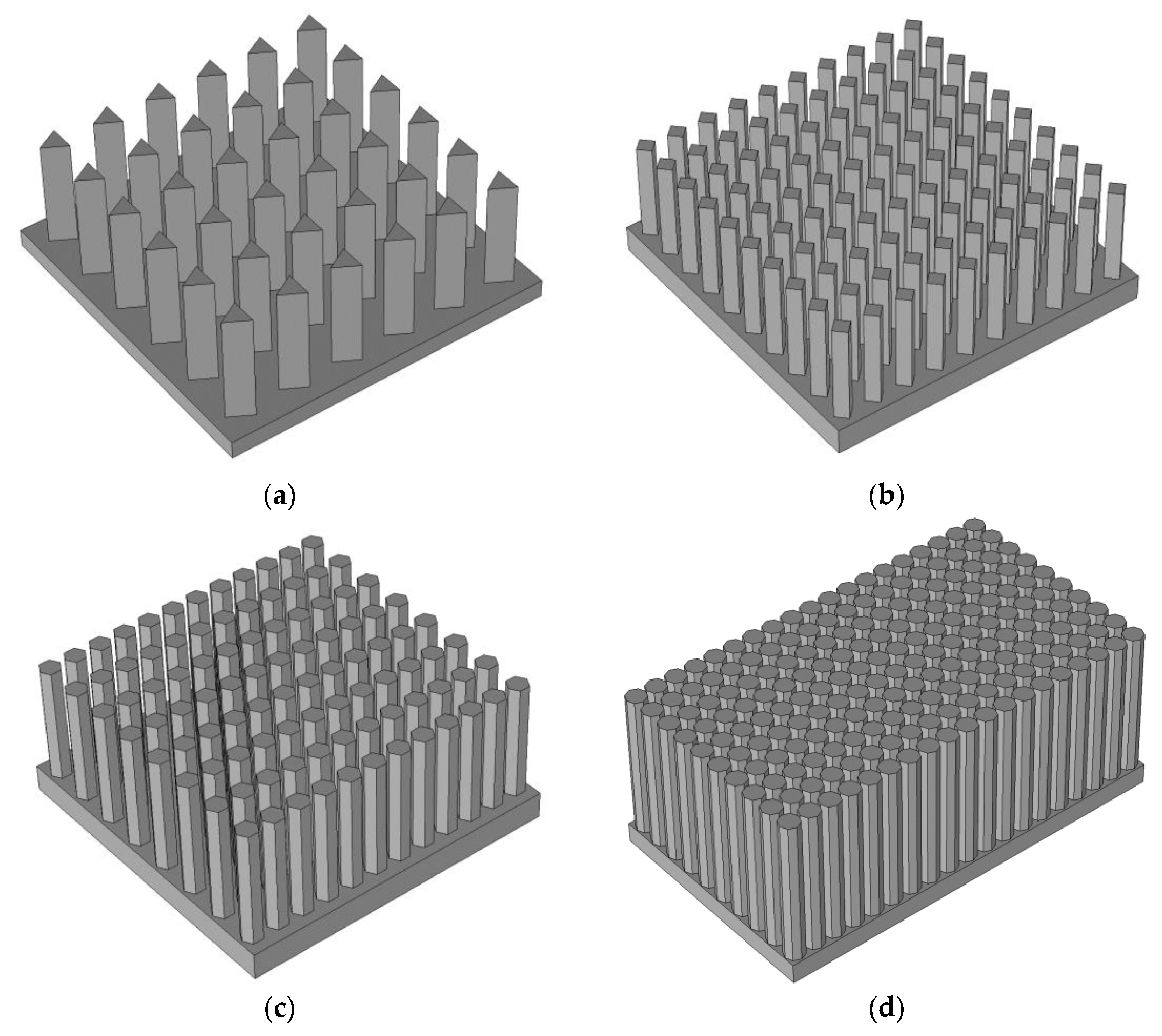
Four isometric views of physical model with different design variables of fins are shown in Figure 12.

The details of the design variables of Figure 12 are shown in

Table 6. Details of the design variables of Figure 12.

Figure ID	${\mathit{t}}_{\mathit{b}}$	$\mathit{h}$	$\mathit{L}$	$\mathit{W}$	$\mathit{r}$	$\mathit{\theta }$	${\mathit{n}}_{\mathit{l}}$	${\mathit{n}}_{\mathit{w}}$	$\mathit{n}$
a	3	18	55	55	2.5	60	6	6	3
b	4	15	50	50	1.5	0	10	10	4
c	5	22	60	60	2	0	12	8	6
d	3	22	60	35	1.5	0	19	10	8

. The heat sink was enhanced with the shown fins.

The heat sink was made of aluminum alloy material. The fluid was air in the optimization. The effects of gravity and radiative heat transfer were neglected. The flow was steady and three dimensional. The governing equations of continuity, momentum, and energy in laminar flow are shown in Equations (20)–(23), respectively.

$$\nabla \cdot \overrightarrow{V}=0$$

(20)

$$\overrightarrow{V}\cdot \nabla \overrightarrow{V}=-\frac{1}{\rho }\nabla P+\nu {\nabla }^2\overrightarrow{V}$$

(21)

$$\overrightarrow{V}\cdot \nabla T=\alpha {\nabla }^{2}T$$

(22)

The energy equation for the solid parts is given by:

$${\nabla }^{2}T=0$$

(23)

where $\overrightarrow{V}$ is the velocity vector showing the flow field, $\rho$ is the density of the fluid, $\nabla P$ is the pressure gradient for convection, ν is the kinematic viscosity, $\alpha$ is the thermal diffusivity, and $T$ is the fluid temperature.

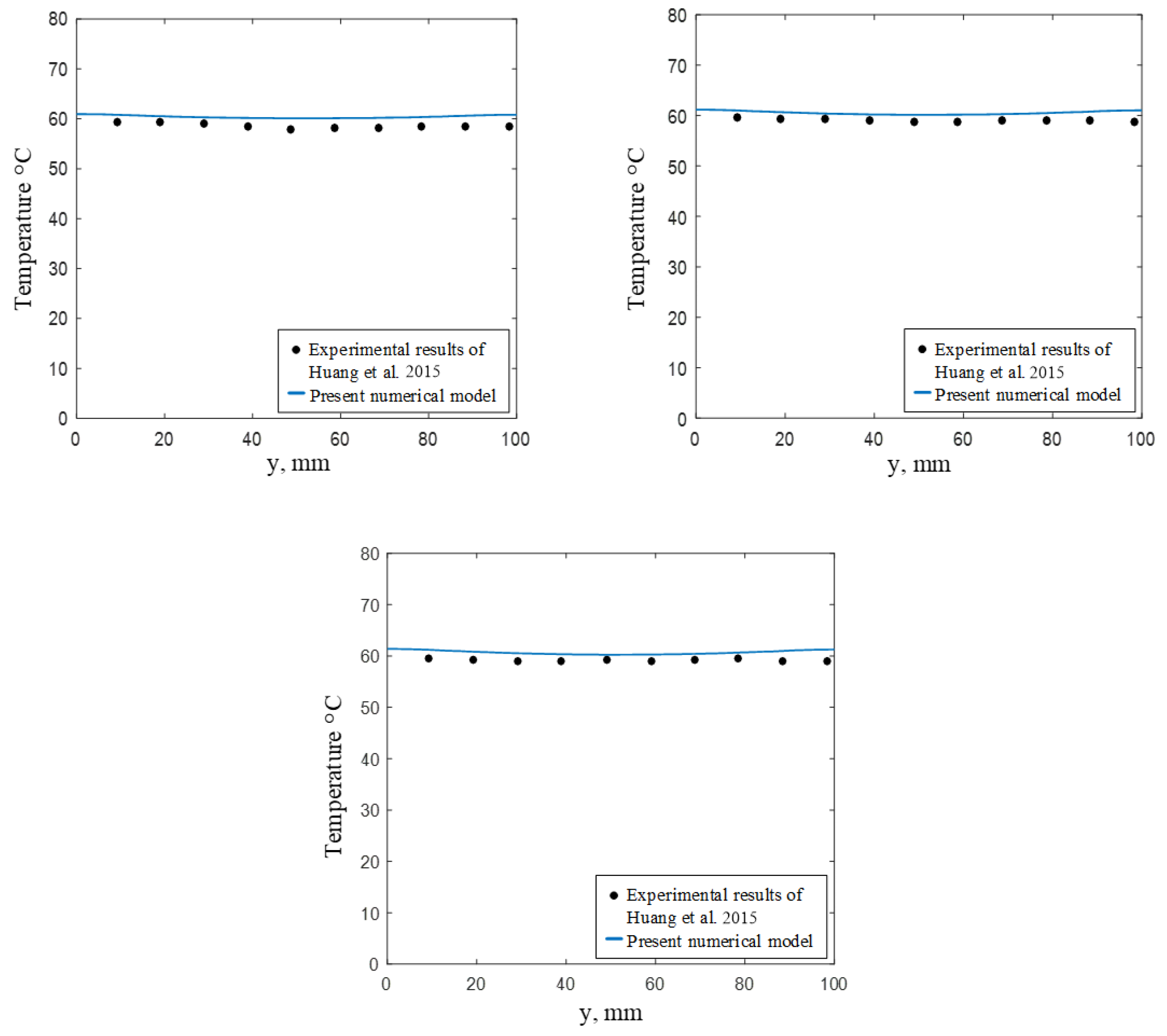
Figure 13a–c shows a comparison between the results of the present numerical model and the experimental data of Huang et al. [36] for different temperature distributions. According to Figure 13, the error between the simulation results of the present model and the experimental results of Huang et al. [36] was acceptable since the average error was approximately 3%. Therefore, the present numerical model was reliable and could be used for the study.

(4) Optimization and results

Generally, the size of the grid affects the accuracy of the model. A fine grid has high accuracy but is computationally expensive, and a coarse grid is computationally cheaper but less accurate. The details of the initial heat sink during the simulation are listed in

Table 7. Geometric description of the initial heat sink.

Iter	${\mathit{t}}_{\mathit{b}}$	$\mathit{h}$	$\mathit{L}$	$\mathit{W}$	$\mathit{r}$	$\mathit{\theta }$	${\mathit{n}}_{\mathit{l}}$	${\mathit{n}}_{\mathit{w}}$	$\mathit{n}$
Values	4 mm	20 mm	60 mm	60 mm	2 mm	45°	9	9	4

.

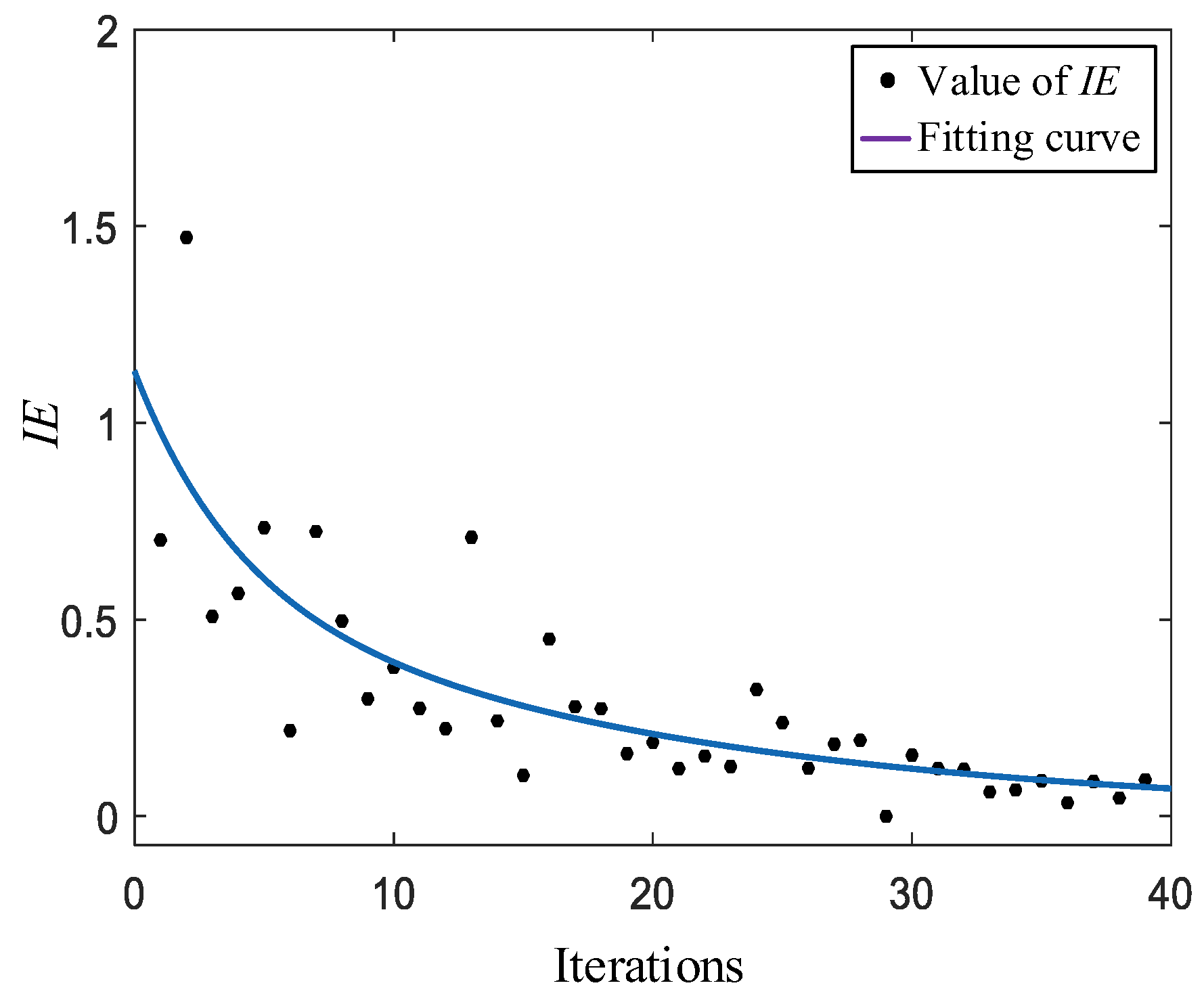
For the initial heat sink FE model, the number of elements was 47,286 for the LFM and 544,521 for the HFM. The maximum number of iterations was set to 40 for optimization of the LFM. The suggested method used a population of 40 particles for the LFM, a mutation rate of 0.1, and a repository size of 200 for both t models. The number selected by the CDE was 40. Let $\omega =$ 0.9, $c_1=$ 1.0, $c_1=$ 2.0. Figure 14 shows the change in IE with the number of iterations in the optimization of the LFM. According to Figure 14, the given stopping criterion was set to $\epsilon$ = 0.2.

As shown in Figure 14, in the initial search stage of the algorithm, the value of IE changed considerably, meaning the particles were searching in the global region. With an increasing number of iterations, the procedure entered the local search stage, and the value IE became small and did not change much.

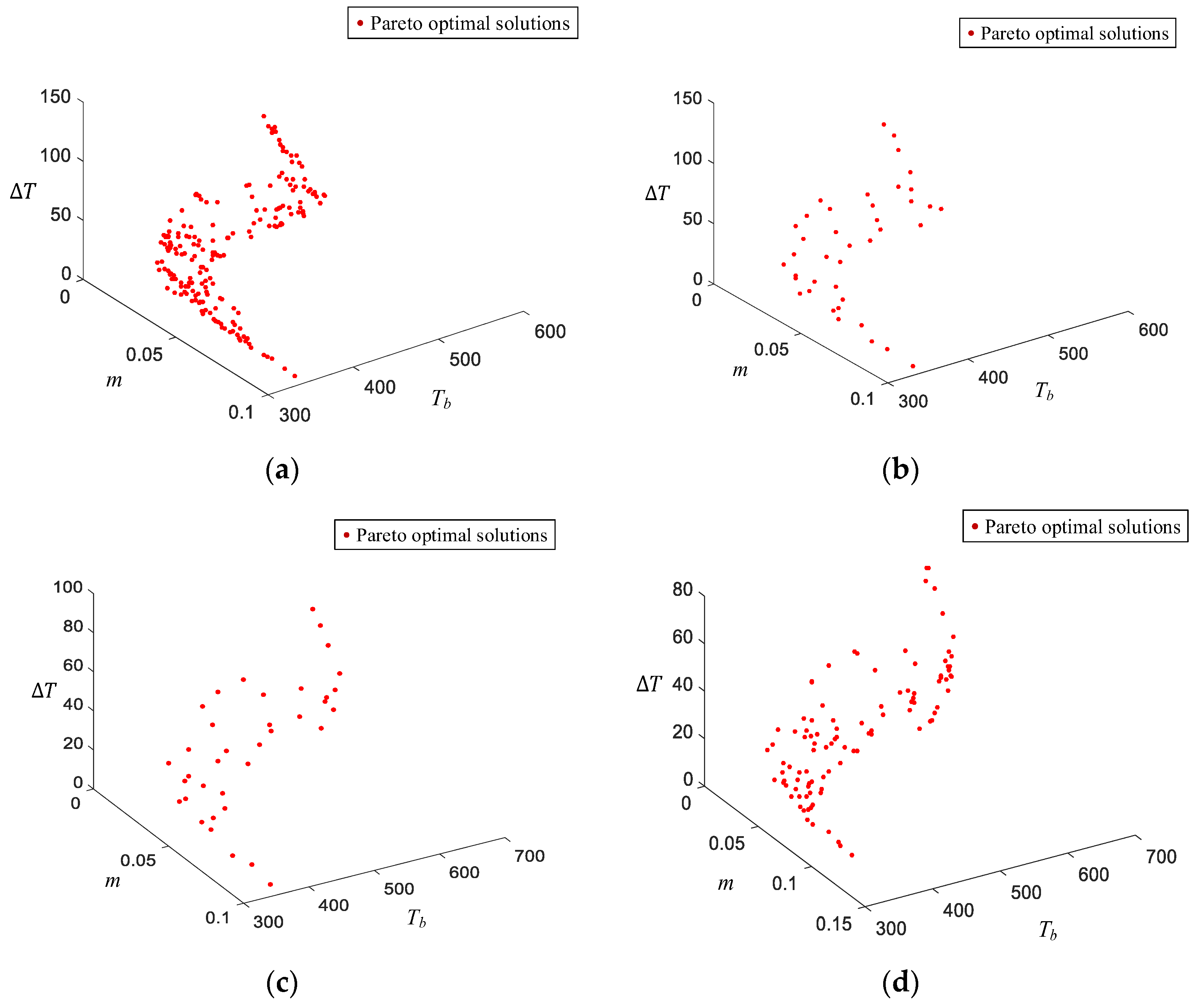
At the beginning of the optimization, compared with the HFM, the relative error $E_{ave}$ of the LHF was 13.58%, suggesting that the two models could be used for optimization. Figure 15 shows the optimization results. In this procedure, the total computational time of the LFM was approximately 40.5 h. A total of 200 Pareto solutions were obtained, as shown in Figure 15a. Figure 15b shows the solutions selected by the CDE. Figure 15c shows the distribution of the Pareto-optimal set of the initial HFM. Comparing Figure 15b,c, it can be seen that the two models were similar. The total computational time of the HFM was approximately 62 h. A total of 102 Pareto solutions were obtained, as shown in Figure 15c. As shown in

Table 8. SP, N, and IE of Pareto optimal solutions metrics and optimization history for heat sink using VFMEM.

Iter	SP	N	IE
1	1.4484	65	0.6684
2	1.6058	83	0.3530
3	1.3922	102	0.1910

, the HFM easily converged after 3 iterations using VFMEM. The updated speed of the Pareto solutions was much faster than that of the LFM during optimization, and the value of IE was relatively small. This means that the optimization might have entered into the local region. Compared with direct optimization, the computational time could theoretically be reduced by 70–80% using the suggested method.

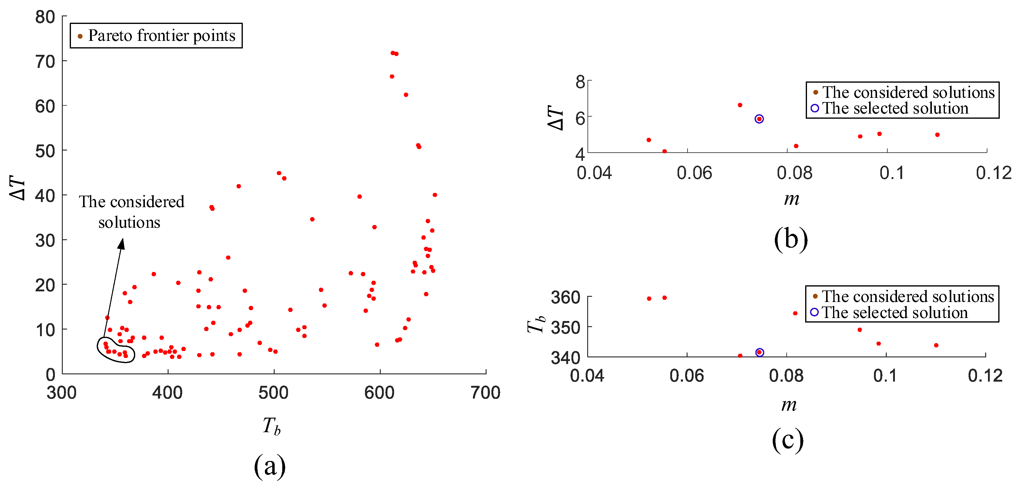
In this optimization, the base temperature and temperature difference were considered more than the mass. There were 102 solutions that could be selected. At first, we considered solutions in which the base temperature and temperature difference were both small. Then, we selected the final design according to the distribution of the considered solutions in the axis of the mass. The solution we selected is shown in Figure 16, and the corresponding design variables are listed in

Table 9. Geometric description of the final heat sink.

Iter	${\mathit{t}}_{\mathit{b}}$	$\mathit{h}$	$\mathit{L}$	$\mathit{W}$	$\mathit{r}$	$\mathit{\theta }$	${\mathit{n}}_{\mathit{l}}$	${\mathit{n}}_{\mathit{w}}$	$\mathit{n}$
Values	4.9 mm	22 mm	60 mm	60 mm	1.87 mm	76.55°	7	6	10

. The temperature distribution of the simulation of the initial and final heat sinks is shown in Figure 17.

The mass of the initial heat sink was 74.7 g and that of the final heat sink was 70.6 g. After optimization, the mass $\left(m\right)$, base temperature ($T_b$) and temperature difference ($\mathsf{\Delta }T$) of the designed optimum heat sink decreased $5.5\%$, $18.5\%$, and $62.0\%$, respectively, compared to the initial design.

6. Conclusions

In this paper, VFMEM was proposed to solve multi-objective optimization and applied to design a polygonal PFHS. The framework of VFMEM was based on MOPSO. Compared with other evolutionary algorithms, the VFO strategy was used. Due to the introduction of LFM and HFM, the number of expensive evaluations was significantly reduced. Compared with other VFO methods, the CDE strategy was suggested and employed to uniformly select points from the Pareto-optimal set. The PT strategy was suggested to transfer the parameters of the selected optimal solutions of the LFM to the HFM so that the HFM could perform a local search at the beginning. Briefly, the LFM was employed to find the global optimal region and the HFM was introduced to find the accurate global optimal solution based on the initial global optimal region. Therefore, the convergence of VFMEM was guaranteed.

To evaluate the performance of VFMEM, some typical nonlinear problems were successfully tested. The results proved that VFMEM can generally converge to the Pareto frontier with a small number of HFM evaluations and can deal with a high dimension, nonlinear, multi-objective problem. Moreover, a heat sink design was successfully solved using the proposed method. The performance of the heat sink was obviously improved using the proposed method. Compared with direct optimization using multi-objective evolutionary algorithms, the optimization cost can be reduced by 70–80% using the suggested method.

7. Further Research

Although VFMEM significantly improved the efficiency of MOSPO, some critical issues need to be further considered. In VFMEM, the similarity of the LFM and HFM should be ensured. If this criterion is not satisfied, convergence might not be achieved. Therefore, the purpose of our next work is how to explore optimization convergence when the similarity of LFM and HFM is not satisfied.

In terms of this issue, we think two important issues should be discussed in future research. The first is how to construct reliable mapping between the LFM and HFM even if the similarity between different fidelity models is weak. In the last 20 years, parameter extraction was mainly used for mapping. The improvement of deep neural networks (DNN), such as the physical informed neural network (PINN) [37,38,39], has provided an alternative method to construct more reliable mapping. Another important issue is improving the performance of heuristic optimization methods. Several kinds of heuristic optimization methods have been proposed [40,41,42,43,44,45], but selecting suitable methods for specific problem remains challenging. Therefore, the focus of our next study is to find an adaptive mechanism to further improve efficiency.

References

1. Husain, A.; Kim, K.-Y. Optimization of a microchannel heat sink with temperature dependent fluid properties. Appl. Therm. Eng. 2008, 28, 1101–1107. [Google Scholar] [CrossRef]
2. Srisomporn, S.; Bureerat, S. Geometrical Design of Plate-Fin Heat Sinks Using Hybridization of MOEA and RSM. IEEE Trans. Compon. Packag. Technol. 2008, 31, 351–360. [Google Scholar] [CrossRef]
3. Bureerat, S.; Srisomporn, S. Optimum plate-fin heat sinks by using a multi-objective evolutionary algorithm. Eng. Optim. 2010, 42, 305–323. [Google Scholar] [CrossRef]
4. Kanyakam, S.; Bureerat, S. Multiobjective Optimization of a Pin-Fin Heat Sink Using Evolutionary Algorithms. J. Electron. Packag. 2012, 134, 021008. [Google Scholar] [CrossRef]
5. Lampio, K.; Karvinen, R. Optimization of convectively cooled heat sinks. Microelectron. Reliab. 2017, 79, 473–479. [Google Scholar] [CrossRef]
6. Huang, H.; Wang, H.; Gu, J.; Wu, Y. High-dimensional model representation-based global sensitivity analysis and the design of a novel thermal management system for lithium-ion batteries. Energy Convers. Manag. 2019, 190, 54–72. [Google Scholar] [CrossRef]
7. Pourfattah, F.; Sabzpooshani, M. On the thermal management of a power electronics system: Optimization of the cooling system using genetic algorithm and response surface method. Energy 2021, 232, 120951. [Google Scholar] [CrossRef]
8. Ramphueiphad, S.; Bureerat, S. Synthesis of multiple cross-section pin fin heat sinks using multiobjective evolutionary algorithms. Int. J. Heat Mass Transf. 2018, 118, 462–470. [Google Scholar] [CrossRef]
9. Vanapalli, S.; Ter Brake, H.J.M.; Jansen, H.V.; Burger, J.F.; Holland, H.J.; Veenstra, T.T.; Elwenspoek, M.C. Pressure drop of laminar gas flows in a microchannel containing various pillar matrices. J. Micromech. Microeng. 2007, 17, 1381–1386. [Google Scholar] [CrossRef]
10. Matsumoto, N.; Tomimura, T.; Koito, Y. Heat Transfer Characteristics of Square Micro Pin Fins under Natural Convection. J. Electron. Cool. Therm. Control 2014, 4, 59–69. [Google Scholar] [CrossRef]
11. Zhao, J.; Huang, S.; Gong, L.; Huang, Z. Numerical study and optimizing on micro square pin-fin heat sink for electronic cooling. Appl. Therm. Eng. 2016, 93, 1347–1359. [Google Scholar] [CrossRef]
12. Thokala, P. Variable Complexity Optimization. Ph.D. Thesis, University of Toronto, Toronto, ON, Canada, 2005. [Google Scholar]
13. Zheng, J.; Qiu, H.; Feng, H. The variable fidelity optimization for simulation-based design: A review. In Proceedings of the 2012 IEEE 16th International Conference on Computer Supported Cooperative Work in Design (CSCWD), Wuhan, China, 23–25 May 2012; IEEE: New York, NY, USA, 2012; pp. 289–294. [Google Scholar]
14. Chang, K.J.; Haftka, R.T.; Giles, G.L.; Kao, P.-J. Sensitivity-based scaling for approximating structural response. J. Aircr. 1993, 30, 283–288. [Google Scholar] [CrossRef]
15. Alexandrov, N.M.; Lewis, R.M. An Overview of First-Order Model Management for Engineering Optimization. Optim. Eng. 2001, 2, 413–430. [Google Scholar] [CrossRef]
16. Gano, S.E.; Renaud, J.E.; Sanders, B. Hybrid Variable Fidelity Optimization by Using a Kriging-Based Scaling Function. AIAA J. 2005, 43, 2422–2433. [Google Scholar] [CrossRef]
17. Bandler, J.W.; Biernacki, R.M.; Chen, S.H.; Grobelny, P.A.; Hemmers, R.H. Space mapping technique for electromagnetic optimization. IEEE Trans. Microw. Theory Tech. 1994, 42, 2536–2544. [Google Scholar] [CrossRef]
18. Feng, F.; Zhang, J.; Zhang, W.; Zhao, Z.; Jin, J.; Zhang, Q.-J. Coarse- and Fine-Mesh Space Mapping for EM Optimization Incorporating Mesh Deformation. IEEE Microw. Wirel. Components Lett. 2019, 29, 510–512. [Google Scholar] [CrossRef]
19. Bandler, J.W.; Ismail, M.A.; Rayas-Sánchez, J.E.; Zhang, Q.J. Neuromodeling of microwave circuits exploiting space-mapping technology. IEEE Trans. Microw. Theory Tech. 1999, 47, 2417–2427. [Google Scholar] [CrossRef]
20. Echeverria, D.; Hemker, P.W. On the Manifold-Mapping Optimization Technique. Modelling, Analysis and Simulation [MAS]; CWI: Hong Kong, China, 2006; R 0612. [Google Scholar]
21. Hu, W.; Enying, L.; Li, G.Y.; Zhong, Z.H. Optimization of sheet metal forming processes by the use of space mapping based metamodeling method. Int. J. Adv. Manuf. Technol. 2007, 39, 642–655. [Google Scholar] [CrossRef]
22. Wang, H.; Fan, T.; Li, G. Reanalysis-based space mapping method, an alternative optimization way for expensive simulation-based problems. Struct. Multidiscip. Optim. 2016, 55, 2143–2157. [Google Scholar] [CrossRef]
23. Eberhart, R.; Kennedy, J. A new optimizer using particle swarm theory. In MHS’95, Proceedings of the Sixth International Symposium on Micro Machine and Human Science, Nagoya, Japan, 4–6 October 1995; IEEE: New York, NY, USA, 1995; pp. 39–43. [Google Scholar]
24. Shi, Y.; Eberhart, R. A modified particle swarm optimizer. In Proceedings of the 1998 IEEE International Conference on Evolutionary Computation Proceedings. IEEE World Congress on Computational Intelligence (Cat. No. 98TH8360), Anchorage, AK, USA, 4–9 May 1998. [Google Scholar]
25. Yang, M.; Wang, H.; Shuai, W.; Deng, X. Thermal optimization of a kirigami-patterned wearable lithium-ion battery based on a novel design of composite phase change materia. Appl. Therm. Eng. 2019, 161, 114141. [Google Scholar] [CrossRef]
26. Ehyaei, M.A.; Ahmadi, A.; Assad, M.E.H.; Salameh, T. Optimization of parabolic through collector (PTC) with multi objective swarm optimization (MOPSO) and energy, exergy and economic analyses. J. Clean. Prod. 2019, 234, 285–296. [Google Scholar] [CrossRef]
27. Jiang, K.; Wang, H.; Zhu, L.; Cheng, C. CPOT: A suitable tool for crack propagation path optimization based on image recognition. Eng. Fract. Mech. 2020, 223, 106765. [Google Scholar] [CrossRef]
28. Luo, X.; Li, E.; Wang, H. A surrogate assisted thermal optimization framework for design of pin-fin heat sink for the platform inertial navigation system. Eng. Optim. 2021, 53, 145–164. [Google Scholar] [CrossRef]
29. Qi, Z.; Wang, H.; He, G.; Li, B.; Li, G. Optimization of a composite pyramidal lattice structure for the auxiliary converter cabinet. Eng. Optim. 2021, 1617–1645. [Google Scholar] [CrossRef]
30. Coello, C.A.C.; Reyes-Sierra, M. Multi-Objective Particle Swarm Optimizers: A Survey of the State-of-the-Art. Int. J. Comput. Intell. Res. 2006, 2, 287–308. [Google Scholar] [CrossRef]
31. Van Veldhuizen, D.A.; Lamont, G.B. Multiobjective evolutionary algorithm research: A history and analysis. In Technical Report TR-98-03; Department of Electrical and Computer Engineering, Graduate School of Engineering, Air Force Institute of Technology, Wright-Patterson AFB: Dayton, OH, USA, 1998. [Google Scholar]
32. Schott, J.R. Fault Tolerant Design Using Single and Multicriteria Genetic Algorithm Optimization (No. AFIT/CI/CIA-95-039); Air Force Inst of Tech Wright-Patterson AFB: Dayton, OH, USA, 1995. [Google Scholar]
33. Zitzler, E.; Deb, K.; Thiele, L. Comparison of Multiobjective Evolutionary Algorithms: Empirical Results. Evol. Comput. 2000, 8, 173–195. [Google Scholar] [CrossRef] [Green Version]
34. Zhang, Q.; Zhou, A.; Zhao, S.; Suganthan, P.N.; Liu, W.; Tiwari, S. Multiobjective Optimization Test Instances for the CEC 2009 Special Session and Competition; Technical Report. 2008. Available online: https://www.al-roomi.org/multimedia/CEC_Database/CEC2009/MultiObjectiveEA/CEC2009_MultiObjectiveEA_TechnicalReport.pdf (accessed on 1 November 2022).
35. Yang, A.; Chen, L.; Xie, Z.; Feng, H.; Sun, F. Constructal heat transfer rate maximization for cylindrical pin-fin heat sinks. Appl. Therm. Eng. 2016, 108, 427–435. [Google Scholar] [CrossRef]
36. Huang, C.-H.; Liu, Y.-C.; Ay, H. The design of optimum perforation diameters for pin fin array for heat transfer enhancement. Int. J. Heat Mass Transf. 2015, 84, 752–765. [Google Scholar] [CrossRef]
37. Yuan, L.; Ni, Y.-Q.; Deng, X.-Y.; Hao, S. A-PINN: Auxiliary physics informed neural networks for forward and inverse problems of nonlinear integro-differential equations. J. Comput. Phys. 2022, 462, 111260. [Google Scholar] [CrossRef]
38. Psaros, A.F.; Kawaguchi, K.; Karniadakis, G.E. Meta-learning PINN loss functions. J. Comput. Phys. 2022, 458, 111121. [Google Scholar] [CrossRef]
39. Wen, Z.; Li, Y.; Wang, H.; Peng, Y. Data-driven spatiotemporal modeling for structural dynamics on irregular domains by stochastic dependency neural estimation. Comput. Methods Appl. Mech. Eng. 2023, 404, 115831. [Google Scholar] [CrossRef]
40. Dulebenets, M.A. A novel memetic algorithm with a deterministic parameter control for efficient berth scheduling at marine container terminals. Marit. Bus. Rev. 2017, 2, 302–330. [Google Scholar] [CrossRef] [Green Version]
41. Kavoosi, M.; Dulebenets, M.A.; Abioye, O.F.; Pasha, J.; Wang, H.; Chi, H. An augmented self-adaptive parameter control in evolutionary computation: A case study for the berth scheduling problem. Adv. Eng. Inform. 2019, 42, 100972. [Google Scholar] [CrossRef]
42. Zhao, H.; Zhang, C. An online-learning-based evolutionary many-objective algorithm. Inf. Sci. 2019, 509, 1–21. [Google Scholar] [CrossRef]
43. Dulebenets, M.A. An Adaptive Polyploid Memetic Algorithm for scheduling trucks at a cross-docking terminal. Inf. Sci. 2021, 565, 390–421. [Google Scholar] [CrossRef]
44. Pasha, J.; Nwodu, A.L.; Fathollahi-Fard, A.M.; Tian, G.; Li, Z.; Wang, H.; Dulebenets, M.A. Exact and metaheuristic algorithms for the vehicle routing problem with a factory-in-a-box in multi-objective settings. Adv. Eng. Inform. 2022, 52, 101623. [Google Scholar] [CrossRef]
45. Rabbani, M.; Oladzad-Abbasabady, N.; Akbarian-Saravi, N. Ambulance routing in disaster response considering variable patient condition: NSGA-II and MOPSO algorithms. J. Ind. Manag. Optim. 2022, 18, 1035. [Google Scholar] [CrossRef]
Figure 1. Description of VFO framework [12].
Sustainability 15 01104 g001
Figure 2. Illustration of the framework of SM [19].
Sustainability 15 01104 g002
Figure 3. Flowchart of MOPSO algorithm.
Sustainability 15 01104 g003
Figure 4. Calculation of distance elimination.
Sustainability 15 01104 g004
Figure 5. The pseudocode of CDE.
Sustainability 15 01104 g005
Figure 6. Procedure of parameter transfer.
Sustainability 15 01104 g006
Figure 7. The framework of VFMEM.
Sustainability 15 01104 g007
Figure 8. The optimization results of ZDT3. (a) The result of optimizing LFM. (b) Solutions selected using CDE. (c) The result of optimizing HFM using VFMEM after 5 iterations. (d) The result of optimizing HFM directly after 100 iterations (MOPSO).
Sustainability 15 01104 g008
Figure 9. The optimization results of UF8. (a) The result of optimizing LFM. (b) Solutions selected using CDE. (c) The result of optimizing HFM using VFMEM after 10 iterations. (d) The result of optimizing HFM directly after 100 iterations.
Sustainability 15 01104 g009
Figure 10. The in-line arrangement a pin fin heat sink model [35]. (a) Top view. (b) Front view. (c) Illustration of fin geometries.
Sustainability 15 01104 g010
Figure 11. Rectangular duct with the heat sink.
Sustainability 15 01104 g011
Figure 12. Isometric views of different pin fin heat sink configurations. (a) Heat sink with triangle fin. (b) Heat sink with quadrilateral fin. (c) Heat sink with hexagon fin. (d) Heat sink with octagon fin.
Sustainability 15 01104 g012
Figure 13. Comparison between the results of the present model and the experimental results of Huang et al. [36] for different temperature distributions.
Sustainability 15 01104 g013
Figure 14. The change in IE with the number of iterations in the optimization of LFM.
Sustainability 15 01104 g014
Figure 15. The optimization result of the heat sink. (a) The Pareto-optimal set of LFM. (b) Solutions selected using CDE. (c) The Pareto-optimal set of HFM in initialization. (d) The Pareto-optimal set of HFM using VFMEM after 3 iterations.
Sustainability 15 01104 g015
Figure 16. Selected PF solutions of different two-combination. (a) The PF solutions according to Δ T and T b . (b) The PF solutions according to Δ T and m . (c) The PF solutions according to T b and m .
Sustainability 15 01104 g016
Figure 17. Temperature distributions of the initial and final heat sinks. (a) Isometric view of the initial and final heat sinks. (b) Top view of the initial and final heat sinks. (c) Front view of the initial and final heat sinks.
Sustainability 15 01104 g017aSustainability 15 01104 g017b