Article

A Short-Term Wind Power Forecasting Model Based on 3D Convolutional Neural Network–Gated Recurrent Unit

School of Geoscience and Technology, Zhengzhou University, Zhengzhou 450001, China
*
Author to whom correspondence should be addressed.
Sustainability 2023, 15(19), 14171; https://doi.org/10.3390/su151914171
Submission received: 11 August 2023 / Revised: 21 September 2023 / Accepted: 21 September 2023 / Published: 25 September 2023
(This article belongs to the Special Issue Renewable Energy Systems and Sustainable Power Systems)

Abstract

:
Enhancing the accuracy of short-term wind power forecasting can be effectively achieved by considering the spatial–temporal correlation among neighboring wind turbines. In this study, we propose a short-term wind power forecasting model based on 3D CNN-GRU. First, the wind power data and meteorological data of 24 surrounding turbines around the target turbine are reconstructed into a three-dimensional matrix and inputted into the 3D CNN and GRU encoders to extract their spatial–temporal features. Then, the power predictions for different forecasting horizons are outputted through the GRU decoder and fully connected layers. Finally, experimental results on the SDWPT datasets show that our proposed model significantly improves the prediction accuracy compared to BPNN, GRU, and 1D CNN-GRU models. The results show that the 3D CNN-GRU model performs optimally. For a forecasting horizon of 10 min, the average reductions in RMSE and MAE on the validation set are about 10% and 11%, respectively, with an average improvement of about 1% in R. For a forecasting horizon of 120 min, the average reductions in RMSE and MAE on the validation set are about 6% and 8%, respectively, with an average improvement of about 14% in R.

1. Introduction

With the increasing global demand for clean and renewable energy, wind power has emerged as the most rapidly growing and widely applied form of energy [1]. According to the latest statistical report released by the Global Wind Energy Council (GWEC) [2], the global wind power capacity witnessed a remarkable surge, with an additional 78 GW added to the grid, in 2022. This exceptional growth rate positions it as the third-highest annual capacity increase ever recorded in the history of the wind power industry. Compared to conventional fossil fuel energy sources, wind power generation offers environmental benefits and energy sustainability [3], which aligns with the goals of reaching peak carbon emissions and achieving carbon neutrality. However, the intermittence, volatility, and high randomness of wind power generation will have a great impact on the grid-connected system [4,5]. Therefore, it is crucial to improve the accuracy and reliability of wind power forecasting to ensure the stable and continuous operation of wind power systems, as well as for economic dispatch and power system operation [6,7].
Wind power is influenced by various factors, including atmospheric conditions, turbine efficiency, maintenance, etc. Generally, wind speed plays a crucial role in the efficiency of converting wind energy into electricity [8], as higher wind speeds correspond to increased wind power generation efficiency. Changes in temperature can alter air density, subsequently affecting turbine performance. Additionally, both turbine efficiency and proper equipment maintenance are significant influencing factors. A comprehensive analysis of the impact of these factors on wind power output is beneficial for forecasting wind power.
Existing wind power forecasting methods can be broadly categorized into three types: physical methods, statistical methods, and machine learning methods [9,10]. Physical methods are based on fluid dynamics principles and the characteristics of wind turbines to model and predict wind power [11], but they have high computational complexity and time consumption, making them suitable for medium-term and long-term forecasts. Statistical methods establish mathematical relationships that capture the historical and future values [12], such as autoregressive integrated moving average (ARIMA) [13], etc. However, these methods may struggle to capture complex nonlinear features and face difficulties in parameter selection. In contrast, machine learning methods have excellent data-processing capabilities and effective extraction of nonlinear features, such as support vector machine (SVM) [14,15], extreme learning machine (ELM) [16,17], and nonlinear autoregressive exogenous (NARX) network [18]. This advancement holds tremendous potential in enhancing the accuracy and reliability of wind power forecasting, showcasing significant advantages. Moreover, with the advancement of machine learning algorithms, the accumulation of data, and the enhancement of computing power, the research on wind power forecasting models is increasingly developing towards better-performing deep neural networks [19,20], including bidirectional long short-term memory (BiLSTM) [21] and deep belief network (DBN) [22,23]. Furthermore, wind power forecasting is subject to various factors such as wind speed, temperature, and more. Due to the complex relationships among these factors, a single prediction model may not capture them comprehensively. Combining multiple models or algorithms into an ensemble model has gained popularity. Ensemble models can effectively balance the different biases and variances among models. Moreover, they can reduce noise and uncertainty by integrating predictions from multiple models, thereby improving prediction accuracy. In reference [24], a model was proposed that combines the power of convolutional neural networks (CNNs) and long short-term memory (LSTM) with the optimization capabilities of coati optimization algorithm (COA) for PV/wind power prediction in smart grid applications. In reference [25], a novel hybrid model was proposed for short-term offshore wind power forecasting, which integrates discrete wavelet transform (DWT), seasonal autoregressive integrated moving average (SARIMA), and LSTM based on deep learning.
The gated recurrent unit (GRU) has displayed impressive capabilities in effectively handling a wide array of temporal data, such as weather forecasting, wind speed forecasting, and wind power forecasting [26,27]. With its unique architecture, the GRU excels at capturing long-term dependencies and patterns within time series. In reference [28], the GRU model was employed to forecast wind power sub-sequences after applying decomposition techniques. In reference [29], the authors demonstrated that the GRU exhibits superior predictive accuracy and offers faster training and lower sensitivity to noise.
In the research on wind power forecasting, CNNs [30,31] have been widely applied for time-series feature extraction. In reference [32], high-level features of wind speed time-series data were extracted using 1D CNN, and through experimental comparisons, it was demonstrated that 1D CNN contributes significantly to improving the predictive capability of the model. In reference [33], a dual-channel CNN was employed to extract waveform features, on a matrix composed of wind speed sub-sequences, thereby demonstrating the feature extraction capability of the CNN. However, there still exist several crucial issues that warrant further investigation. Limited by the inherent structure of the networks, the wind power forecasting model based on a 1D CNN or 2D CNN is unable to consider the spatial correlation of data when dealing with sequential data. In other words, they cannot handle spatial–temporal sequences, leading to the neglect of spatial features in the data. This limitation hampers the accuracy and reliability of wind power forecasts. Therefore, it is necessary to develop other forecasting approaches that can overcome these shortcomings and fully leverage the spatial information present in the data. Thus, 3D CNNs have been proposed for extracting spatial–temporal features from video data [34]. In reference [35], an RNN and 3D CNN were employed for mobile traffic prediction, demonstrating the model’s effectiveness in capturing spatial and temporal features to improve prediction accuracy.
Additionally, neighboring wind turbines exhibit similar variations in power curves with certain time delays [36]. Considering time delays in wind power forecasting is essential. In order to address the issue of time delays, it is possible to leverage existing spatial–temporal correlations and incorporate future information into the forecasting model. This entails not only relying on current observed data but also considering the historical data and spatial relationships, to better capture the fluctuation patterns in wind power generation. By integrating spatial–temporal correlations into the forecasting model, more accurate predictions of future power variations can be achieved, thereby improving the precision of the forecasts. However, previous wind power forecasting models typically only considered the relevant wind power and meteorological information from a single site, focusing solely on the temporal correlation of wind power [37], while ignoring the effective utilization of nearby turbines’ wind power and meteorological data.
Therefore, the goal of this study is to establish a hybrid model based on a 3D CNN and GRU for short-term wind power forecasting. Specifically, this article charts the following: Firstly, a data cleaning strategy is established, and meteorological factors with strong correlation are selected using the Pearson correlation coefficient method and random forest model. Next, a three-dimensional matrix is constructed using historical power data from multiple turbines around the target turbine as the input for the 3D CNN and GRU. Finally, the model outputs the predicted wind power values for different forecasting horizons.
The organization of this paper is structured as follows: Section 2 describes the methods employed and presents the structure of the proposed model. Section 3 contains information about the dataset used, the prediction process, and the selected model evaluation metrics. Section 4 analyzes and discusses the results. Finally, Section 5 concludes this study.

2. Methods

2.1. Three-Dimensional Convolutional Neural Network

Convolutional neural networks can be divided into 1D CNNs [38], 2D CNNs [39], and 3D CNNs. The CNN performs feature extraction on input data through operations such as convolution, activation functions, and pooling [40,41]. Compared to the 1D CNN and 2D CNN, the convolution kernel of the 3D CNN not only slides in the spatial dimension but also in the temporal dimension (Figure 1). This allows the 3D CNN to better preserve time information while extracting spatial features, thereby considering both the local and global characteristics of the features [42,43]. The utilization of the 3D CNN enables a more effective capturing of the correlations between wind speed and other features across various locations and time points [44]. The calculation formula is as follows:
v i j x y z = f p = 0 P i 1 q = 0 Q i 1 r = 0 R i 1 ω i j m p q r v ( i 1 ) m ( x + p ) ( y + q ) ( z + r ) + b i j
where v i j x y z is the value at position (x, y, z) of the j-th feature map of the i-th layer; f is the activation function; m indexes over the set of feature maps in the (i − 1)-th layer connected to the current feature map, and is the (p, q, r)-th value of the kernel connected to the m-th feature map in the previous laver; P i , Q i , a n d   R i are the length, width, and height of the convolution kernel, respectively; and b i j is the bias term of the current feature map.

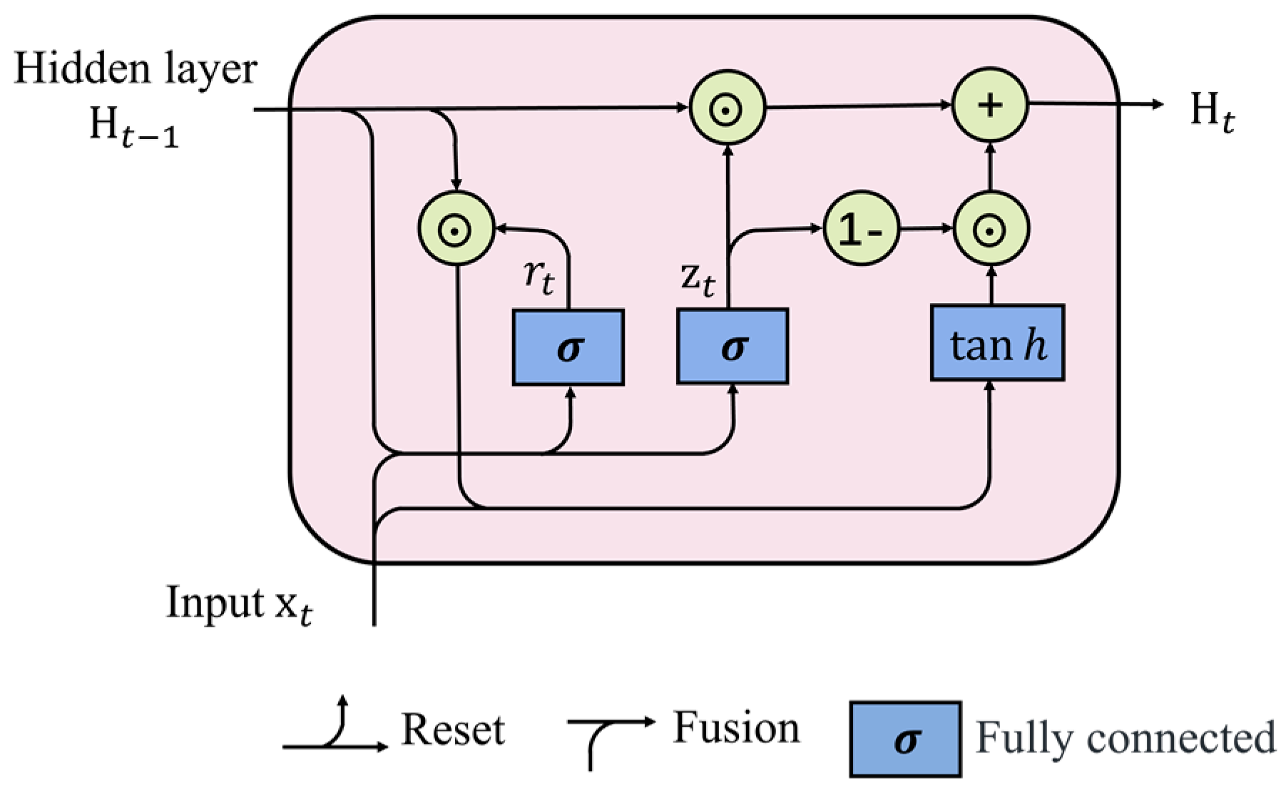
2.2. Gated Recurrent Unit

The GRU architecture is an improved type of recurrent neural network (RNN) designed to address the issues of gradient vanishing and exploding that arise with increasing network layers and iterations in traditional RNNs [45]. As a variant of LSTM [46,47], the GRU reduces the number of gates and possesses a more simplified structure [48]. It utilizes the update gate and the reset gate to determine whether to retain or discard the hidden state information from the previous time step [49], using a Sigmoid function to output values between 0 and 1 that determine the degree of information retention. By selectively updating and forgetting information, the GRU is capable of capturing long-term dependencies in the data more effectively. The unit structure of the GRU is shown in Figure 2. Assuming that x t is the input and h t is the output of the hidden layer, the GRU calculates h t with the following formula:
z t = σ W z x t + U z h t 1
r t = σ W r x t + U r h t 1
h t ~ = tan h r t ° U h t 1 + W x t
h t = 1 z t ° h t ~ + z t ° h t 1
where z t and r t are the update gate and the reset gate, respectively; h t ~ is the sum of the input x t and the output h t 1 of the previous hidden layer; σ is a sigmoid function; t a n h is a hyperbolic tangent function; U z , W z , U r , W r , U , and W are training parameter matrices; and z t ° h t 1 is the composite relation of z t and h t 1 .

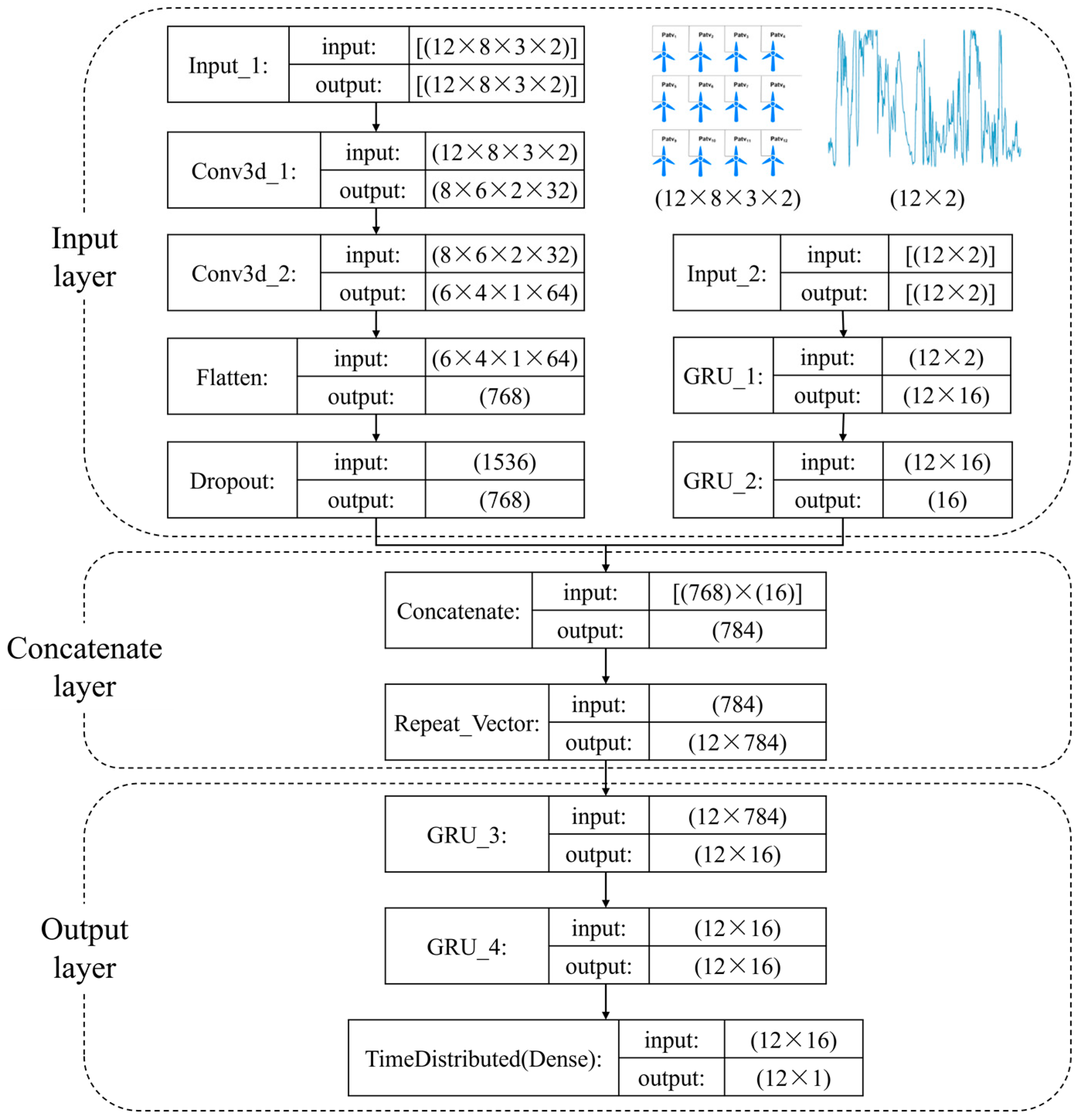
2.3. The 3D CNN-GRU Model

The structure and parameters of the 3D CNN-GRU network model constructed in this study are shown in Figure 3. The input layer receives historical power and meteorological data, which are inputted into the 3D CNN and GRU encoders to extract the spatial–temporal features of power and wind speed. The concatenate layer concatenates the respective extraction results in series in the concatenate layer. The output layer predicts the power values through the GRU decoder and full connection layer. Specifically, the encoder 3D CNN module consists of two convolutional layers, which are sized at 5 × 3 × 2 and 3 × 3 × 2, respectively, with 32 convolution kernels each; the time step size is 1. The GRU module comprises two GRU layers with 16 hidden units. The final prediction of power is outputted as 12 × 1 through the “Time-Distributed” layer in Keras, corresponding to different forecasting horizons.

3. Experiment and Analysis

3.1. Datasets and Experimental Environment

The experiment utilized the SDWPT [50] wind power forecasting datasets obtained from the Supervisory Control and Data Acquisition (SCADA) system of a wind farm. These datasets comprise key external features and basic internal feature parameters of 134 wind turbines, with a sampling interval of 10 min. The meanings of some selected parameters are shown in Table 1. In this study, data from 25 turbines were selected for power prediction research, and their relative spatial positions are shown in Figure 4. Following data preprocessing, a total of 7331 samples were obtained, with the first 5865 samples used as the training set and the last 1466 samples used as the validation set.
The prediction task in this study was executed in the Python3.8 environment, with the experimental hardware configuration consisting of an Intel Core i5-10300H CPU, 16 GB RAM, and GeForce GTX 1650.

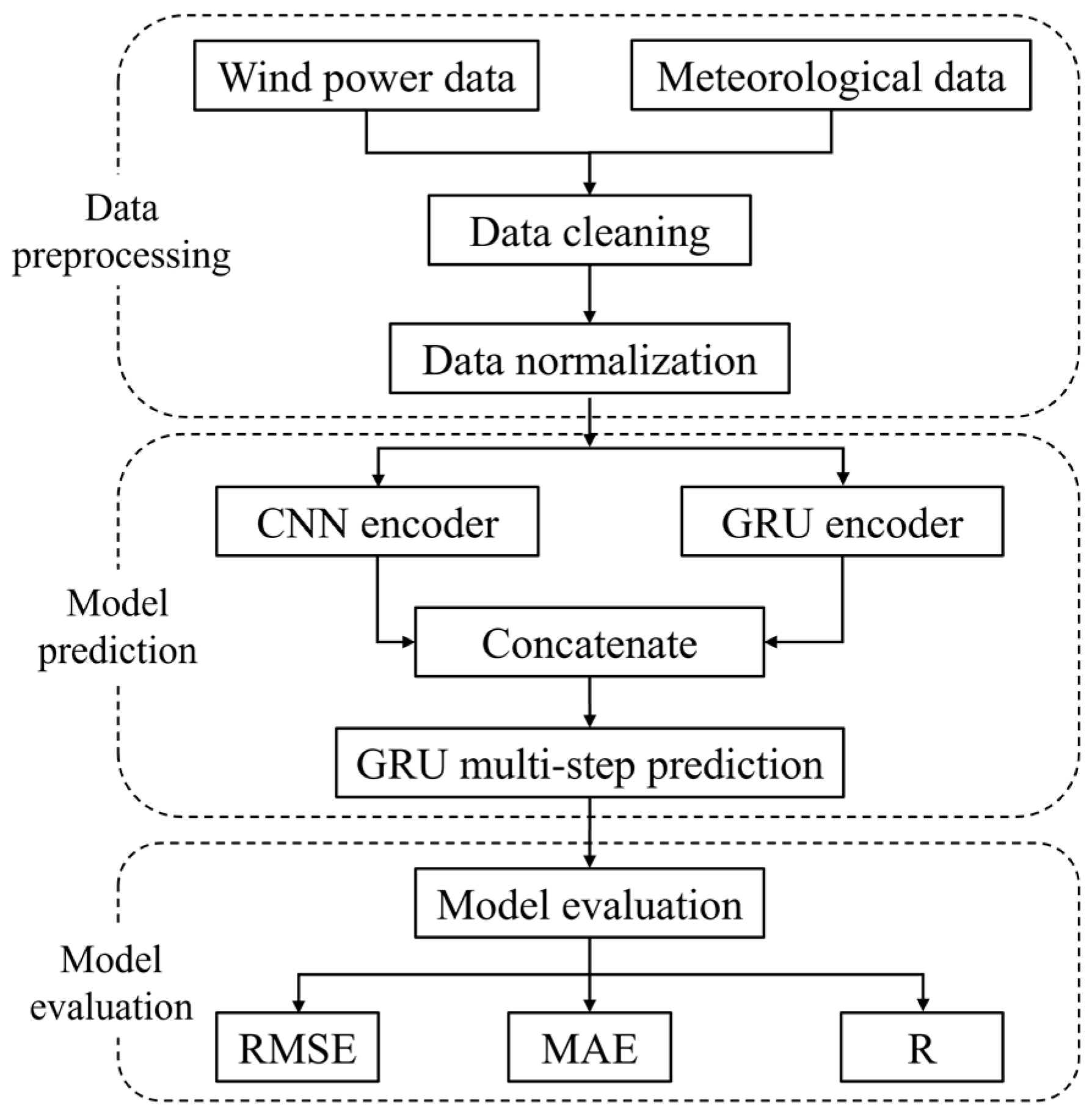
3.2. Flow of Experiment

The process of predicting using the 3D CNN-GRU model constructed is shown in Figure 5. The process mainly consists of three modules: data preprocessing, model prediction, and model evaluation. The data preprocessing module performs data cleaning and normalization on the raw wind power data and meteorological data, reconstructing data suitable for model prediction. The model prediction module employs the constructed 3D CNN-GRU model for wind power forecasting. The model evaluation module selects model evaluation metrics for comparative analysis of the models.

3.3. Data Preprocessing

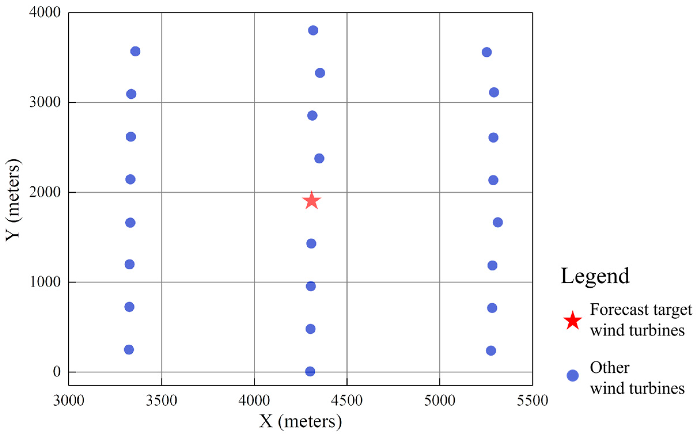
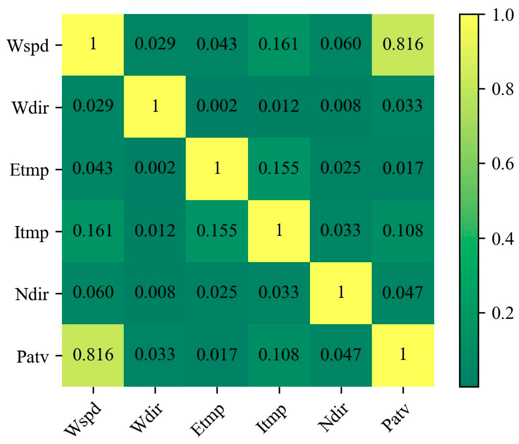
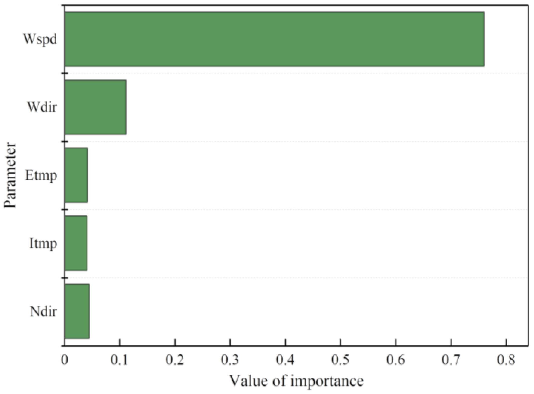
3.3.1. Feature Parameter Selection

Selecting appropriate feature parameters as model inputs can improve the accuracy of the prediction model, as well as enhance its interpretability [51]. This study used the Pearson correlation coefficient (PCC) and feature importance values to facilitate the selection of feature parameters that possess the highest information content and predictive capability. The selected meteorological parameters included Wspd, Wdir, Etmp, Itmp, and Ndir. Firstly, based on the calculation of PCC values, the correlation between parameters was visualized. The results are shown in Figure 6. Among them, the PCC value between wind speed and wind power is 0.816, indicating a significantly higher correlation compared to other parameters. Generally, a PCC value greater than 0.8 can be defined as a strong correlation.
Furthermore, to analyze the complex nonlinear relationship between different parameters and wind power, feature importance values were calculated using a random forest model. The random forest model effectively captures the nonlinear relationships among parameters by employing a combinatorial strategy of decision trees. As shown in Figure 7, it is evident that wind speed has the highest importance value among the five selected parameters. Therefore, wind speed and wind power were chosen as the feature inputs.

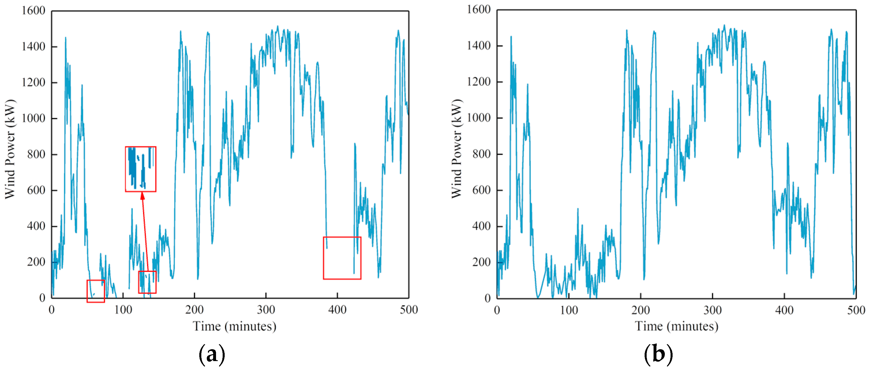
3.3.2. Data Reconstruction

Due to various physical factors, signal interference, and errors during wind turbine operation, data may contain outliers and missing values. To improve data quality and reliability, preprocessing operations are required before data reconstruction. Firstly, to address the issue of data noise, a threshold was set to filter out usable data. Then, the data were segmented according to time steps, with a maximum allowable number of missing values set at 24. Each time step was checked for the presence of consecutive missing values. Finally, the filtered unusable data were removed, and the missing values were interpolated using a moving average interpolation method. The effect of data preprocessing on partial power series data is shown in Figure 8.
The processed time series data were then reconstructed into a three-dimensional matrix, where the first dimension represents time, the second dimension represents the turbine’s location information, and the third dimension represents local features (wind speed and power vectors).
Furthermore, in order to address the differences in dimension and value range among diverse features, and to ensure the trainability and optimization of the model, the data were subjected to min-max normalization. This technique not only eliminates the variations in scale but also brings the data to a standardized range suitable for effective training and optimization of the model.

3.4. Performance Indices

To evaluate the predictive ability, accuracy, and reliability of the model, three metrics, namely root-mean-square error (RMSE), mean absolute error (MAE), and correlation coefficient (R), were selected to comprehensively analyze the differences and correlations between the predicted results and the actual values. RMSE was used to measure the average deviation between the predicted values and the real values, reflecting the overall fluctuation of the prediction results. MAE was used to measure the average absolute error between the predicted values and the real values, revealing the overall bias of the prediction results. Both metrics indicate higher accuracy with smaller values. R was used to measure the linear correlation between the predicted values and the real values, ranging from −1 to 1. A value closer to 1 indicates a stronger correlation between the predicted and actual values, indicating a better predictive performance of the model. Conversely, a weaker correlation suggests a poorer predictive performance. These metrics are defined as follows:
R M S E = 1 n i = 1 n y i y i 2
M A E = 1 n i = 1 n y i y i
R = i = 1 n y i y i ¯ y i y i ¯ i = 1 n y i y i ¯ 2 i = 1 n y i y i ¯ 2
where n , y i , and y i are the sample size, the real value of power, and the predicted value of power, respectively, and y i ¯ and y i ¯ are the averages of the real value of power and the predicted value of power, respectively.

4. Results and Analysis

4.1. Analysis of Prediction Results

In this study, backpropagation neural network (BPNN), GRU, and 1D CNN-GRU models were selected as comparative models to validate the effectiveness of the 3D CNN-GRU model. BPNN is a commonly used classical model that utilizes a backpropagation algorithm during training to minimize errors; it utilizes a single hidden layer in its architecture. GRU is a single-gated recurrent unit model. The 1D CNN-GRU model combines a one-dimensional convolutional neural network with gated recurrent units. To ensure the fairness of the experimental comparison, each model shared the same set of hyperparameters, as shown in Table 2. The selected four models were experimentally applied to the wind power datasets, with forecasting horizons set at 10 min, 40 min, 80 min, and 120 min. Various evaluation metrics were computed for quantitative analysis. The comparative results of the model performance are shown in Table 3.
Figure 9 shows a validation performance comparison of the four models, indicating that the proposed model outperforms the other three comparative models with a significant decrease in both RMSE and MAE and an improvement in R. This demonstrates that the predictions obtained from the 3D CNN-GRU model exhibit overall smaller fluctuations and biases, showcasing superior predictive performance.
Quantitative analysis was conducted on the results of the validation set, revealing the superior performance of the 3D CNN-GRU model. Specifically, in comparison to the BPNN, GRU, and 1D CNN-GRU models, the RMSE decreased, respectively, by approximately: 14.56%, 9.41%, and 7.85% for a forecasting period of 10 min; 9.96%, 8.23%, and 6.06% for a forecasting period of 40 min; 8.39%, 7.45%, and 5.03% for a forecasting period of 80 min; and 6.97%, 6.00%, and 4.38% for a forecasting period of 120 min. Similarly, in comparison to the BPNN, GRU, and 1D CNN-GRU models, the MAE decreased, respectively, by approximately: 14.63%, 11.41%, and 7.58% for a forecasting period of 10 min; 12.24%, 10.02%, and 7.71% for a forecasting period of 40 min; 12.32%, 9.25%, and 6.54% for a forecasting period of 80 min; and 11.39%, 7.83%, and 5.49% for a forecasting period of 120 min. Additionally, in terms of R, there was an average increase of approximately: 1% for a forecasting period of 10 min; 3% for a forecasting period of 40 min; 6% for a forecasting period of 80 min; and finally, 14% for a forecasting period of 120 min.
To further analyze the reasons behind the improved wind power, forecasting accuracy through the combination of 3D CNN and GRU was evaluated. Among the four models investigated in the experiment, the BPNN model exhibited the lowest performance, effectively highlighting the efficacy of deep learning models. Comparative analysis of 1D CNN-GRU, 3D CNN-GRU, and GRU models revealed that the inclusion of any type of CNN in the standalone GRU model improves predictive accuracy. In the comparative analysis of 1D CNN-GRU and 3D CNN-GRU models, the 3D CNN outperformed the 1D CNN in extracting spatial–temporal features, while the 1D CNN could only capture local features from time series data. Taking into account the spatial–temporal correlation between neighboring turbines, incorporating spatial information on predictive factors can improve the accuracy of predictions.
Additionally, as the forecasting horizon extended, there was a slight decrease in the rate of reduction in RMSE when comparing a forecasting horizon of 120 min to 10 min. This can be attributed to the heightened sensitivity of RMSE to large errors. When there is a significant deviation between the predicted and real values, the RMSE value increases significantly, thereby reducing the improvement rate. Moreover, in multi-step forecasting, the accumulation of initial errors and uncertainties over an extended time range is one of the reasons for the decline in the RMSE improvement rate. Additionally, in terms of the correlation coefficient R, the decline rate of the 3D CNN-GRU model’s performance is significantly lower than that of other models as the forecasting horizon increases. When extending from 10 min to 120 min, the validation set R of the BPNN, GRU, and 1D CNN-GRU reduced by 25.24%, 22.76%, and 25.50%, respectively, while the validation set R of the 3D CNN-GRU only decreased by 14.82%.

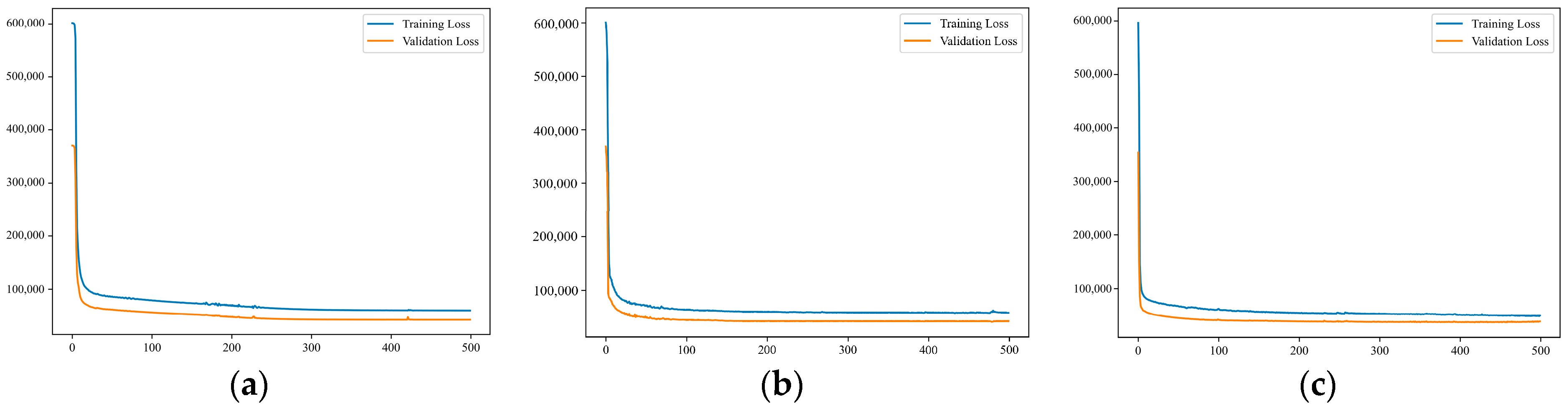
4.2. Evaluation of Model Performance

Mean-squared error (MSE) was chosen as the loss function to comprehensively evaluate the training process and optimization effect of the predictive models. The loss functions for the GRU, 1D CNN-GRU, and 3D CNN-GRU are shown in Figure 10. It is evident that the 3D CNN-GRU model demonstrates faster convergence and lower values of the loss function for both the training and validation sets. This indicates its ability to swiftly learn the patterns and characteristics of the data, effectively capturing the underlying patterns and features present in the training data.

5. Conclusions

This study presents a short-term wind power forecasting model based on a 3D CNN, and GRU, which were applied to the SDWPT wind power forecasting datasets for experimental analysis. By incorporating the spatial–temporal correlation among neighboring turbines, the wind power and meteorological data from 24 surrounding turbines of the target turbine were reconstructed into a three-dimensional matrix as input. By utilizing the 3D CNN and GRU encoders, spatial–temporal features were extracted. Then, the GRU decoder was utilized to predict power values for different forecasting horizons. The main findings are as follows:
(1)
Effectively utilizing the spatial–temporal correlation among neighboring turbines can improve the accuracy of wind power forecasting. Comparative analysis between the 1D CNN-GRU and 3D CNN-GRU models revealed that the 3D CNN demonstrates a more comprehensive ability to extract spatial–temporal features from input data, surpassing the limitations of the 1D CNN.
(2)
The proposed 3D CNN-GRU demonstrated superior predictive performance in this study. Comparative analysis with the BPNN, GRU, and 1D CNN-GRU models demonstrated that the proposed model achieved better predictive performance. For a forecasting horizon of 10 min, the average reductions in RMSE and MAE on the validation set were about 10% and 11%, respectively, with an average improvement in R of about 1%. For a forecasting horizon of 120 min, the average reductions in RMSE and MAE on the validation set were about 6% and 8%, respectively, with an average improvement in R of about 14%.
The problem of error accumulation in multi-step predictions was not further addressed in this study. In future research, it is recommended that the adoption of ensemble learning techniques should be considered, such as stacked ensemble. Additionally, to obtain a more comprehensive view of how the variables are related to wind/turbine data, employing diverse methods is recommended.

Author Contributions

All authors made valuable contributions to this paper. Conceptualization, X.H. and Y.Z.; resources, X.H., Y.Z. and S.L.; formal analysis, Y.Z. and J.L.; methodology, X.H. and S.L.; data curation, X.H., X.Z. and S.L.; software, X.H.; validation, X.H., Y.Z., S.L. and X.Z.; visualization, X.H. and S.L.; writing—original draft preparation, X.H., Y.Z. and J.L.; writing—review and editing, X.H., Y.Z. and J.L. All authors have read and agreed to the published version of the manuscript.

Funding

This research was funded by the National Social Science Foundation of China under a Major Project, and solicited by the National Office of Philosophy and Social Science, under the title of Interdisciplinary Research on the Theory and Methodology of Geo-environmental Analysis in the Era of Big Data (No. 20&ZD138).

Institutional Review Board Statement

Not applicable.

Informed Consent Statement

Not applicable.

Data Availability Statement

Data are available in a publicly accessible repository.

Conflicts of Interest

The authors declare no conflict of interest.

References

  1. Ma, Z.; Mei, G. A hybrid attention-based deep learning approach for wind power prediction. Appl. Energy 2022, 323, 119608. [Google Scholar] [CrossRef]
  2. Yin, S.; Liu, H. Wind power prediction based on outlier correction, ensemble reinforcement learning, and residual correction. Energy 2022, 250, 123857. [Google Scholar] [CrossRef]
  3. Xiong, B.; Meng, X.; Xiong, G. Multi-branch wind power prediction based on optimized variational mode decomposition. Energy Rep. 2022, 8, 11181–11191. [Google Scholar] [CrossRef]
  4. Liu, M.; Ding, L.; Bai, Y. Application of hybrid model based on empirical mode decomposition, novel recurrent neural networks and the ARIMA to wind speed prediction. Energy Convers. Manag. 2021, 233, 113917. [Google Scholar] [CrossRef]
  5. Ahn, E.; Hur, J. A short-term forecasting of wind power outputs using the enhanced wavelet transform and arimax techniques. Renew. Energy 2023, 212, 394–402. [Google Scholar] [CrossRef]
  6. Ding, Y.; Chen, Z.; Zhang, H. A short-term wind power prediction model based on CEEMD and WOA-KELM. Renew. Energy 2022, 189, 188–198. [Google Scholar] [CrossRef]
  7. Xing, Z.; Qu, B.; Liu, Y. Comparative study of reformed neural network based short-term wind power forecasting models. IET Renew. Power Gener. 2022, 16, 885–899. [Google Scholar] [CrossRef]
  8. Lopez-Villalobos, C.A.; Martínez-Alvarado, O.; Rodriguez-Hernandez, O. Analysis of the influence of the wind speed profile on wind power production. Energy Rep. 2022, 8, 8079–8092. [Google Scholar] [CrossRef]
  9. Li, J.; Zhang, S.; Yang, Z. A wind power forecasting method based on optimized decomposition prediction and error correction. Electr. Power Syst. Res. 2022, 208, 107886. [Google Scholar] [CrossRef]
  10. Ji, T.; Wang, J.; Li, M. Short-term wind power forecast based on chaotic analysis and multivariate phase space reconstruction. Energy Convers. Manag. 2022, 254, 115196. [Google Scholar] [CrossRef]
  11. Wang, Y.; Zou, R.; Liu, F. A review of wind speed and wind power forecasting with deep neural networks. Appl. Energy 2021, 304, 117766. [Google Scholar] [CrossRef]
  12. Peng, X.; Wang, H.; Lang, J.; Li, W.; Xu, Q.; Zhang, Z. EALSTM-QR: Interval wind-power prediction model based on numerical weather prediction and deep learning. Energy 2021, 220, 119692. [Google Scholar] [CrossRef]
  13. Yuan, X.; Tan, Q.; Lei, X. Wind power prediction using hybrid autoregressive fractionally integrated moving average and least square support vector machine. Energy 2017, 129, 122–137. [Google Scholar] [CrossRef]
  14. Liu, M.; Cao, Z.; Zhang, J. Short-term wind speed forecasting based on the Jaya-SVM model. Int. J. Electr. Power Energy Syst. 2020, 121, 106056. [Google Scholar] [CrossRef]
  15. Li, Z.; Luo, X.; Liu, M. Wind power prediction based on EEMD-Tent-SSA-LS-SVM. Energy Rep. 2022, 8, 3234–3243. [Google Scholar] [CrossRef]
  16. Shan, J.; Wang, H.; Pei, G. Research on short-term power prediction of wind power generation based on WT-CABC-KELM. Energy Rep. 2022, 8, 800–809. [Google Scholar] [CrossRef]
  17. Hua, L.; Zhang, C.; Peng, T. Integrated framework of extreme learning machine (ELM) based on improved atom search optimization for short-term wind speed prediction. Energy Convers. Manag. 2022, 252, 115102. [Google Scholar] [CrossRef]
  18. López, G.; Arboleya, P. Short-term wind speed forecasting over complex terrain using linear regression models and multivariable LSTM and NARX networks in the Andes Mountains, Ecuador. Renew. Energy 2022, 183, 351–368. [Google Scholar] [CrossRef]
  19. González Sopeña, J.M.; Pakrashi, V.; Ghosh, B. A benchmarking framework for performance evaluation of statistical wind power forecasting models. Sustain. Energy Technol. Assess. 2023, 57, 103246. [Google Scholar] [CrossRef]
  20. Xing, Z.; He, Y. Multi-modal multi-step wind power forecasting based on stacking deep learning model. Renew. Energy 2023, 215, 118991. [Google Scholar] [CrossRef]
  21. Jaseena, K.U.; Kovoor, B.C. Decomposition-based hybrid wind speed forecasting model using deep bidirectional LSTM networks. Energy Convers. Manag. 2021, 234, 113944. [Google Scholar] [CrossRef]
  22. He, J.; Yu, C.; Li, Y.; Xiang, H. Ultra-short term wind prediction with wavelet transform, deep belief network and ensemble learning. Energy Convers. Manag. 2020, 205, 112418. [Google Scholar] [CrossRef]
  23. Hu, S.; Xiang, Y.; Huo, D. An improved deep belief network based hybrid forecasting method for wind power. Energy 2021, 224, 120185. [Google Scholar] [CrossRef]
  24. Abou Houran, M.; Salman Bukhari, S.M.; Zafar, M.H. COA-CNN-LSTM: Coati optimization algorithm-based hybrid deep learning model for PV/wind power forecasting in smart grid applications. Appl. Energy 2023, 349, 121638. [Google Scholar] [CrossRef]
  25. Zhang, W.; Lin, Z.; Liu, X. Short-term offshore wind power forecasting—A hybrid model based on Discrete Wavelet Transform (DWT), Seasonal Autoregressive Integrated Moving Average (SARIMA), and deep-learning-based Long Short-Term Memory (LSTM). Renew. Energy 2022, 185, 611–628. [Google Scholar] [CrossRef]
  26. Yu, M.; Niu, D.; Gao, T. A novel framework for ultra-short-term interval wind power prediction based on RF-WOA-VMD and BiGRU optimized by the attention mechanism. Energy 2023, 269, 126738. [Google Scholar] [CrossRef]
  27. Ahmad, T.; Zhang, D. A data-driven deep sequence-to-sequence long-short memory method along with a gated recurrent neural network for wind power forecasting. Energy 2022, 239, 122109. [Google Scholar] [CrossRef]
  28. Wu, H.; Guo, C.; Su, C. Combined Prediction Method for Short-Term Wind Power Based on EEMD-GRU-MC. South. Power Syst. Technol. 2023, 17, 66–73. [Google Scholar] [CrossRef]
  29. Kisvari, A.; Lin, Z.; Liu, X. Wind power forecasting—A data-driven method along with gated recurrent neural network. Renew. Energy 2021, 163, 1895–1909. [Google Scholar] [CrossRef]
  30. Ren, J.; Yu, Z.; Gao, G. A CNN-LSTM-LightGBM based short-term wind power prediction method based on attention mechanism. Energy Rep. 2022, 8, 437–443. [Google Scholar] [CrossRef]
  31. Yildiz, C.; Acikgoz, H.; Korkmaz, D. An improved residual-based convolutional neural network for very short-term wind power forecasting. Energy Convers. Manag. 2021, 228, 113731. [Google Scholar] [CrossRef]
  32. Lawal, A.; Rehman, S.; Alhems, L.M. Wind Speed Prediction Using Hybrid 1D CNN and BLSTM Network. IEEE Access 2021, 9, 156672–156679. [Google Scholar] [CrossRef]
  33. Bi, G.; Zhao, X.; Li, L. Dual-model Decomposition CNN-LSTM Integrated Short-term Wind Speed Forecasting Model. Acta Energiae Solaris Sin. 2023, 44, 191–197. [Google Scholar] [CrossRef]
  34. Tran, D.; Bourdev, L.; Fergus, R. Learning spatiotemporal features with 3d convolutional networks. In Proceedings of the IEEE International Conference on Computer Vision, Santiago, Chile, 7–13 December 2015; pp. 4489–4497. [Google Scholar]
  35. Huang, C.; Chiang, C.; Li, Q. A study of deep learning networks on mobile traffic forecasting. In Proceedings of the 2017 IEEE 28th Annual International Symposium on Personal, Indoor, and Mobile Radio Communications (PIMRC), Montreal, QC, Canada, 8–13 October 2017; IEEE: Piscataway, NJ, USA, 2017; pp. 1–6. [Google Scholar]
  36. Lydia, M.; Kumar, S.S.; Selvakumar, A.I. A comprehensive review on wind turbine power curve modeling techniques. Renew. Sustain. Energy Rev. 2014, 30, 452–460. [Google Scholar] [CrossRef]
  37. Yu, G.; Liu, C.; Tang, B. Short term wind power prediction for regional wind farms based on spatial-temporal characteristic distribution. Renew. Energy 2022, 199, 599–612. [Google Scholar] [CrossRef]
  38. Cho, K.; Van Merrienboer, B.; Gulcehre, C. Learning Phrase Representations using RNN Encoder-Decoder for Statistical Machine Translation. arXiv 2014, arXiv:1406.1078. [Google Scholar] [CrossRef]
  39. Xie, Y.; Sun, W.; Ren, M. Stacking ensemble learning models for daily runoff prediction using 1D and 2D CNNs. Expert Syst. Appl. 2023, 217, 119469. [Google Scholar] [CrossRef]
  40. Duan, J.; Chang, M.; Chen, X. A combined short-term wind speed forecasting model based on CNN–RNN and linear regression optimization considering error. Renew. Energy 2022, 200, 788–808. [Google Scholar] [CrossRef]
  41. Shen, Z.; Fan, X.; Zhang, L. Wind speed prediction of unmanned sailboat based on CNN and LSTM hybrid neural network. Ocean Eng. 2022, 254, 111352. [Google Scholar] [CrossRef]
  42. Wang, X.; Du, Y.; Chen, D. Constructing better prototype generators with 3D CNNs for few-shot text classification. Expert Syst. Appl. 2023, 225, 120124. [Google Scholar] [CrossRef]
  43. Fu, H.; Shao, Z.; Fu, P. Combining ATC and 3D-CNN for reconstructing spatially and temporally continuous land surface temperature. Appl. Earth Obs. Geoinf. 2022, 108, 102733. [Google Scholar] [CrossRef]
  44. Zhu, X.; Liu, R.; Chen, Y. Wind speed behaviors feather analysis and its utilization on wind speed prediction using 3D-CNN. Energy 2021, 236, 121523. [Google Scholar] [CrossRef]
  45. Han, L.; Jing, H.; Zhang, R. Wind power forecast based on improved Long Short Term Memory network. Energy 2019, 189, 116300. [Google Scholar] [CrossRef]
  46. Hochreiter, S.; Schmidhuber, J. Long Short-Term Memory. Neural Comput. 1997, 9, 1735–1780. [Google Scholar] [CrossRef]
  47. Shahid, F.; Zameer, A.; Muneeb, M. A novel genetic LSTM model for wind power forecast. Energy 2021, 223, 120069. [Google Scholar] [CrossRef]
  48. Xiao, Y.; Zou, C.; Chi, H. Boosted GRU model for short-term forecasting of wind power with feature-weighted principal component analysis. Energy 2023, 267, 126503. [Google Scholar] [CrossRef]
  49. Chen, B.; Xie, D.; Huang, R. Research on IGBT aging prediction method based on adaptive VMD decomposition and GRU-AT model. Energy Rep. 2023, 9, 1432–1446. [Google Scholar] [CrossRef]
  50. Zhou, J.; Lu, X. SDWPF: A Dataset for Spatial Dynamic Wind Power Forecasting Challenge at KDD Cup 2022. In Proceedings of the 28th ACM SIGKDD Conference on Knowledge Discovery and Data Mining (Baidu KDD Cup 2022), Washington, DC, USA, 14–18 August 2022; ACM: New York, NY, USA, 2022. [Google Scholar]
  51. Zhang, Y.; Li, R. Short term wind energy prediction model based on data decomposition and optimized LSSVM. Sustain. Energy Technol. Assess. 2022, 52, 102025. [Google Scholar] [CrossRef]
Figure 1. Three-dimensional convolution kernel sliding process in time dimension.
Sustainability 15 14171 g001
Figure 2. The unit structure of the GRU.
Sustainability 15 14171 g002
Figure 3. The structure and parameters of the 3D CNN-GRU network model.
Sustainability 15 14171 g003
Figure 4. The relative spatial positions of turbines.
Sustainability 15 14171 g004
Figure 5. Prediction flow chart based on 3D CNN-GRU model.
Sustainability 15 14171 g005
Figure 6. Matrix plot of Pearson correlation coefficient.
Sustainability 15 14171 g006
Figure 7. Parameter importance diagram.
Sustainability 15 14171 g007
Figure 8. Data preprocessing on partial power series: (a) before processing, the red boxes represent outliers and missing values; (b) after processing.
Sustainability 15 14171 g008
Figure 9. Validation performance comparison of models: (a) RMSE; (b) MAE.
Sustainability 15 14171 g009
Figure 10. Loss functions of the models: (a) GRU; (b) 1D CNN-GRU; (c) 3D CNN-GRU.
Sustainability 15 14171 g010
Table 1. Partial parameters and meanings.
ParameterMeaning
Patv(kW)Active power of the turbine
Wspd (m/s)Wind speed recorded by the anemometer
Wdir (°)Angle between the wind direction and the position of turbine nacelle
Etmp (°C)Temperature of the surrounding environment
Itmp (°C)Temperature inside the turbine nacelle
Ndir (°)Nacelle direction, i.e., the yaw angle of the nacelle
Table 2. Hyperparameter settings of the model.
HyperparameterValue/Type
Training set5865 (80%)
Validation set1466 (20%)
Learning rate0.001
Loss functionMSE
OptimizerAdam
Table 3. Performances of the four models.
Forecasting Horizon
(Minutes)
ModelTrainingValidation
RMSEMAERRMSEMAER
10BPNN146.944108.7350.939119.68385.0000.943
GRU140.686100.2070.942112.87681.9070.949
1D CNN-GRU135.10297.0010.950111.85678.9370.953
3D CNN-GRU124.31489.8060.958102.26072.5640.958
40BPNN223.622167.7180.850186.243136.6950.852
GRU218.304162.2690.853182.727133.3280.856
1D CNN-GRU211.920156.3200.871178.278127.2820.869
3D CNN-GRU193.004141.8430.898167.692119.9630.885
80BPNN272.859207.1820.779231.514172.8320.775
GRU269.815203.5370.783229.153166.9920.780
1D CNN-GRU261.962196.0330.798224.691162.3060.785
3D CNN-GRU228.893172.0500.855212.079151.5450.827
120BPNN309.944237.1070.726265.385200.5560.705
GRU306.594232.3790.730262.648192.8020.733
1D CNN-GRU295.010223.7770.739256.278188.8530.710
3D CNN-GRU267.036202.5600.808246.886177.7080.816
Disclaimer/Publisher’s Note: The statements, opinions and data contained in all publications are solely those of the individual author(s) and contributor(s) and not of MDPI and/or the editor(s). MDPI and/or the editor(s) disclaim responsibility for any injury to people or property resulting from any ideas, methods, instructions or products referred to in the content.

