Grid-Following Inverter-Based Resource: Numerical State–Space Modeling

Abstract

In the pursuit of a sustainable electric power system, the integration of renewable energy sources and distributed energy resources is gradually replacing traditional power generation. These new resources are integrated into the grid via inverters, which, despite their efficient performance, present dynamic challenges to the power grid when implemented on a large scale. To maintain grid stability and ensure effective regulation during abnormal operations, various modeling techniques are necessary; while the dynamics of inverter-based resources (IBRs) are traditionally modeled by transfer functions, this paper sheds light on differential-algebraic equations (DAEs) modeling and numerical integration methods. The inherent limitations of transfer function modeling stem from its restricted applicability, as it is exclusively suitable for linear and time-invariant systems. In contrast, the nonlinear DAEs of the IBR system can be converted into a state–space form, which offers a versatile framework for modeling, evaluating, and designing a diverse array of systems. In addition to being compatible with time-varying systems and multiple-input multiple-output systems, the state–space technique may incorporate saturation and dead zone characteristics into the dynamic model. Our research focuses on IBR modeling in a grid-following scheme, which is current-controlled and synchronized to the grid by a phase-locked loop (PLL). The presented state–space model consists of the inverter, grid, control, and designed PLL. Beyond the discussion of its application to IBRs, the presented method holds the potential to solve a wide range of DAEs. The proposed model is compared with a benchmarked system.

1. Introduction

Growing concerns about environmental pollution, the depletion of fossil fuels, and global warming all serve as powerful motivators for a rapid transition away from conventional energy supplies toward renewable energy resources, which play a crucial role in promoting sustainability [1]. As the passive distribution system is being activated, the migration process necessitates reconstructing the existing grid infrastructure. In the traditional grid, the power flow is central and unidirectional. Scatteredly installed distributed generators (DG) in the grid change these two grid characteristics. In recent years, the idea of a microgrid has become increasingly prevalent in power systems. The U.S. Department of Energy defines the microgrid as a collection of interconnected loads and distributed energy resources operating within properly specified electrical limits as a single controllable entity with respect to the grid and capable to operate in both grid-connected and island modes [2]. Dispersed generation throughout the grid reduces losses and improves reliability.

While active distribution systems provide numerous solutions, they also bring some difficulties that researchers and the industry must overcome. The significant challenge is in comprehending the system dynamics through system modeling. The focus of this research is on inverter-based resources (IBRs), which are extensively employed in active distribution systems. An AC microgrid’s power inverter connections can be categorized as either grid-following or grid-forming, depending on which role the inverters are designed to perform [3,4].

Grid-following power inverters are mostly constructed to supply power to a grid that is already energized. They can be modeled as a high-impedance, parallel current source connected to the grid. In this application, it is important to note that this current source should be precisely synchronized with the ac voltage at the connection point so that the active and reactive power exchanged with the grid can be controlled accurately. Due to this, the grid-following technique is incapable of operating autonomously in Island Mode. The control configuration of this connection is applied to the active and reactive power. The grid-forming technique is analogous to an ideal ac voltage source with a low output impedance. Each of the integrated inverters of such a connection is considered an independent source of power. Furthermore, the connected inverter is accountable for determining the voltage and frequency of the local supplied area. Therefore, the grid-forming scheme has the ability to operate independently in an Island Mode. The system voltage and frequency are used to govern the configuration of this connection.

Inverters must be synchronized with the grid for all types of DERs. Grid synchronization, in fact, consists in the real-time monitoring of system variables. Due to the fact that system states may change owing to failures, disturbances, resonances, or even load changes, instantaneous system monitoring is needed [5,6,7,8]. Furthermore, both inverter connection and disconnection must be performed while monitoring the grid states at the point of common coupling to ensure that the system is operating in accordance with the grid requirement codes [9].

The phase-locked loop, or PLL, is the predominant mechanism for synchronizing converters. Two methods are used for integrating the PLL with the grid: open-loop and closed-loop [10]. While the open-loop connection has many applications, the closed-loop connection has gained popularity due to its greater precision. For applications requiring a three-phase grid-connected converter, the synchronous reference frame PLL (SRF-PLL) is the most prevalent type of PLL [11]. The PLL device can estimate from the connection point the voltage magnitude, frequency, and phase angle. The SRF-PLL’s mechanism proceeds as follows [12]: the PLL transforms the three-phase grid voltage $V_{abc}$ into the $dq$-frame voltage $V_{dq}$, which is based on the rotating frame and appears as DC. The PI controller suppresses the $V_q$ to zero and aligns the grid voltage to the d-axis. The output of the PI controller and the integrator eventually provides the grid voltage phase angle, which is likewise sent back to the Park transformation utilized in the process.

The SRF-PLL operates effectively while operating in a balanced state, but fails to perform well when operating in an abnormal or imbalanced state. Reference [13] proposes a decoupled double synchronous reference frame PLL for power converters control. In their work, the authors enable the PLL to extract the grid voltage’s fundamental component during the inclusion of the distortion components. Other researchers in the field have proposed improved versions of, or whole new replacements for, the standard PLL [14,15,16,17,18,19,20]. This paper implements the SRF-PLL and develops its controller to accommodate unbalanced components.

Similar to synchronous machines, inverters can be modeled via ordinary differential equations (ODEs). The majority of the controllers can be modeled with ODEs if time-dependent delays are approximated with lags or simply disregarded [21]. Power system dynamics are generally driven by two types of state variables: slow and fast. The slow-state variables involve big-time constants, whereas the fast-state variables involve small-time constants. The dynamical variation of the slow-state variables is small and significant, and can therefore be overlooked. The dynamics of the fast-state variables, on the other hand, are serious and must be considered in system modeling. Due to the mixture of such variables, the studied model is composed of a set of nonlinear differential-algebraic equations (DAEs).

Modeling the dynamics of a wide variety of power system applications is a function that can be performed with the DAE system. The numerical solution of the DAE system can be approached using either explicit or implicit integration schemes, depending on the element of the system being analyzed. The explicit integration scheme is renowned for its ease of use and applicability to a wide range of applications. The implicit scheme can achieve the same result as the explicit scheme, but it necessitates the inclusion of two matrices that pertain to the system under consideration.

The state–space modeling of a grid-connected inverter is introduced in [22]. Expanding on this existing work, our research substantially contributes to the field by detailing the derivation process of the state–space representation. Furthermore, we have incorporated a comprehensive methodology for numerically solving the state–space equations. The advanced understanding and tools provided through this research are expected to aid in the design, analysis, and optimization of grid-connected inverter systems. The following summarizes this paper’s contribution:

• Model an inverter-based resource coupled to a grid-following scheme using differential-algebraic equations.
• Introduce a versatile synchronous reference frame phase-locked loop (SRF-PLL) that is designed to be able to operate in the existence of the imbalanced component.
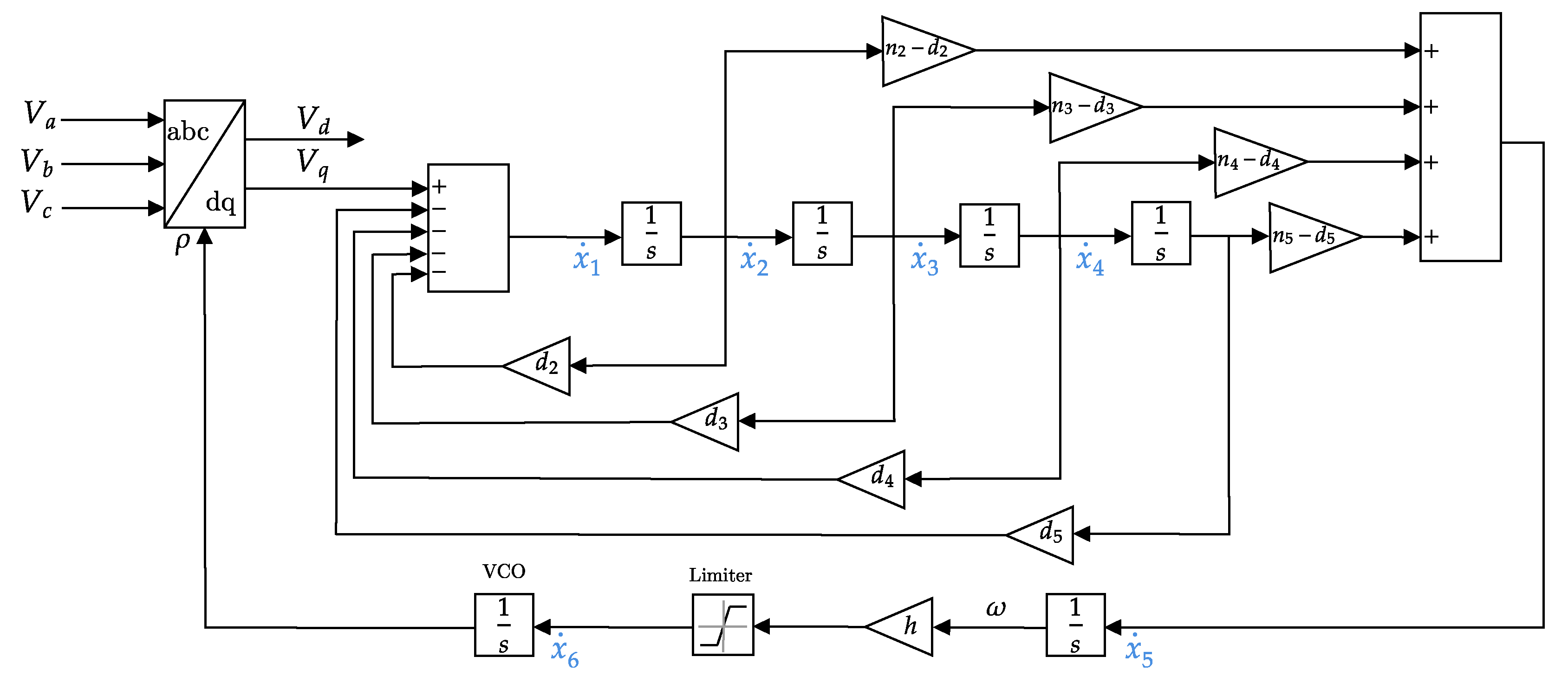
• Demonstrate how to convert the transfer functions of the system into state–space form. The procedure, albeit implemented with the IBR model, is generic and can be employed with other dynamical applications.
• Integrate and simulate the proposed model using the Forward Euler Method (FEM), the Backward Euler Method (BEM), and the Implicit Trapezoidal Method (ITM).

2. Grid-Following Frequency Inverter System

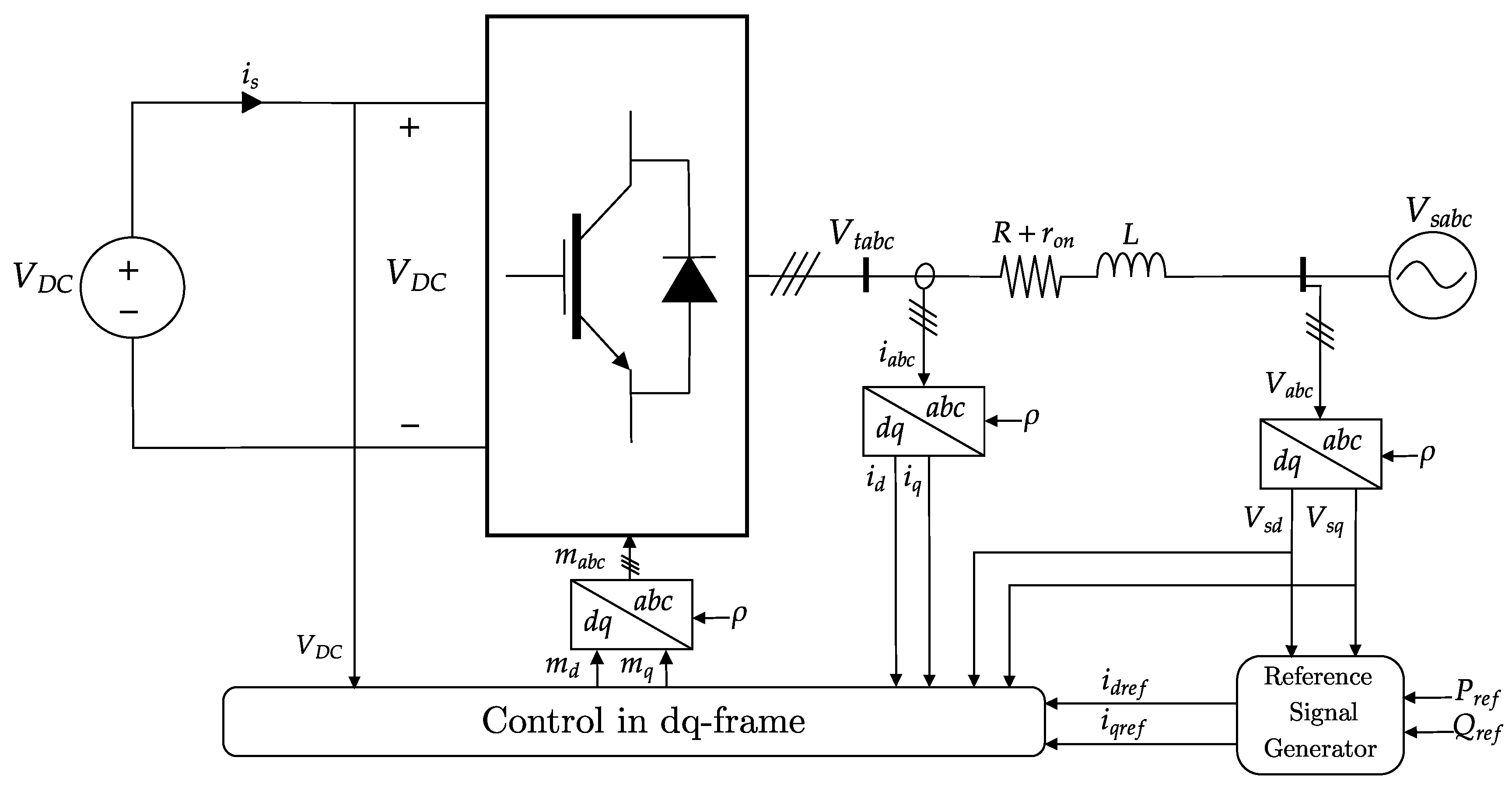
Inverters facilitate the transformation of electrical energy from DC to AC. On the DC side, the inverter is typically linked to a DC source, or alternatively, another power electronic system. These can be effectively modeled as a combination of a DC source, a capacitor, and a current source. The latter is a representation of the power loss attributed to the converter. The losses incurred when the inverter is in an operational state manifest as resistors on the AC side of the system.

In the context of this research, we delve into the dynamics of a three-phase inverter that is engaged in the supply of a stiff, balanced grid operating at a constant frequency. On the AC side, each phase of the inverter is interfaced with an ideal voltage source via a series RL branch, a configuration that creates an inductive–resistive pathway. The point at which these phases are collectively coupled with the grid is known as the Point of Common Coupling (PCC), and the system is illustrated in Figure 1.

The role of the grid-following inverter is to "follow" the grid’s behavior by adjusting its output voltage and frequency to align with those of the AC microgrid. This is achieved through a mechanism known as the Phase-Locked Loop (PLL), which enables synchronization between the inverter’s voltage and frequency and those of the grid. The PLL plays a crucial role in maintaining grid stability and ensuring the efficient operation of the inverter with the grid.

2.1. dq-Frame

To control the grid-following converter-interfaced system, it is more practical to reduce the system’s structure and convert the actual three-phase frame to either $\alpha \beta$-frame or $dq$-frame. For large-scale systems, the latter is more convenient as its control is DC and it does not require a large bandwidth. The following equation converts the three-phase frame to $dq$-frame

$$\left[\begin{array}{c}{f}_d\left(t\right)\hfill \\ f_q\left(t\right)\hfill \end{array}\right]=\frac{2}{3}\left[\begin{array}{c}cos\left[\rho \left(t\right)\right]cos\left[\rho \left(t\right)-\frac{2\pi }{3}\right]cos\left[\rho \left(t\right)-\frac{4\pi }{3}\right]\hfill \\ sin\left[\rho \left(t\right)\right]sin\left[\rho \left(t\right)-\frac{2\pi }{3}\right]sin\left[\rho \left(t\right)-\frac{4\pi }{3}\right]\hfill \end{array}\right]\left[\begin{array}{c}{f}_a\left(t\right)\hfill \\ f_b\left(t\right)\hfill \\ f_c\left(t\right)\hfill \end{array}\right],$$

(1)

where $f\left(\right)$ can represent the voltage and the current. $\rho$ is the PCC voltage angle that allows for the frame conversion and is achieved from PLL. The $abc$-frame can be retrieved as follows:

$$\left[\begin{array}{c}{f}_a\left(t\right)\hfill \\ f_b\left(t\right)\hfill \\ f_c\left(t\right)\hfill \end{array}\right]=\left[\begin{array}{cc}cos\left[\rho \right(t\left)\right]& sin\left[\rho \right(t\left)\right]\\ cos\left[\rho \left(t\right)-\frac{2\pi }{3}\right]& sin\left[\rho \left(t\right)-\frac{2\pi }{3}\right]\\ cos\left[\rho \left(t\right)-\frac{4\pi }{3}\right]& sin\left[\rho \left(t\right)-\frac{4\pi }{3}\right]\end{array}\right]\left[\begin{array}{c}{f}_d\left(t\right)\hfill \\ f_q\left(t\right)\hfill \end{array}\right].$$

(2)

2.2. Grid Modeling

This research considers an inverter that is connected to a stiff grid; the voltage is assumed to be balanced with constant frequency. The three-phase voltages are expressed as follows:

$$\begin{array}{c}{V}_{sa}\left(t\right)={\widehat{V}}_{s}cos\left({\omega }_{0}t+{\theta }_0\right),\hfill \\ V_{sb}\left(t\right)={\widehat{V}}_{s}cos\left({\omega }_{0}t+{\theta }_0-\frac{2\pi }{3}\right),\hfill \\ V_{sc}\left(t\right)={\widehat{V}}_{s}cos\left({\omega }_{0}t+{\theta }_0-\frac{4\pi }{3}\right),\hfill \end{array}$$

(3)

where ${\widehat{V}}_s$ is the peak value of the line-to-neutral voltage, ${\omega }_0$ is the grid angular frequency, and ${\theta }_0$ is the initial phase angle. The grid is modeled in $abc$-frame as follows:

$$L\frac{d}{dt}\left[\begin{array}{c}{i}_a\left(t\right)\hfill \\ i_b\left(t\right)\hfill \\ i_c\left(t\right)\hfill \end{array}\right]=-(R+r_{on})\left[\begin{array}{c}{i}_a\left(t\right)\hfill \\ i_b\left(t\right)\hfill \\ i_c\left(t\right)\hfill \end{array}\right]+\left[\begin{array}{c}{V}_{ta}\left(t\right)\hfill \\ V_{tb}\left(t\right)\hfill \\ V_{tc}\left(t\right)\hfill \end{array}\right]-\left[\begin{array}{c}{V}_{sa}\left(t\right)\hfill \\ V_{sb}\left(t\right)\hfill \\ V_{sc}\left(t\right)\hfill \end{array}\right].$$

(4)

Using (1), the grid can be expressed in $dq$-frame as follows:

$$\begin{array}{c}L\frac{d{i}_d}{dt}=L\omega \left(t\right)i_q-\left(R+r_{on}\right)i_d+V_{td}-{\widehat{V}}_{s}cos\left({\omega }_{0}t+{\theta }_0-\rho \right),\hfill \\ L\frac{d{i}_q}{dt}=-L\omega \left(t\right)i_d-\left(R+r_{on}\right)i_q+V_{tq}-{\widehat{V}}_{s}sin\left({\omega }_{0}t+{\theta }_0-\rho \right),\hfill \\ \frac{d\rho }{dt}=\omega \left(t\right).\hfill \end{array}$$

(5)

For this system, the control inputs $V_{td}$, $V_{tq}$, and $\omega$ determine the dynamics of the state variables $i_d$, $i_q$, and $\rho$. It can be noticed that the system includes nonlinear components that are $\omega i_d$, $\omega i_q$, $cos({\omega }_{0}t+{\theta }_0-\rho )$, $sin({\omega }_{0}t+{\theta }_0-\rho )$. With the help of the Phase-Locked Loop (PLL), the system phase angle can be accurately detected. $\rho$ represents the detected angle from PLL. With $\rho ={\omega }_{0}t+{\theta }_0$, the complexity of the nonlinearity disappeared

$$\begin{array}{c}L\frac{d{i}_d}{dt}=L{\omega }_0{i}_q-\left(R+r_{on}\right)i_d+V_{td}-V_{sd},\hfill \\ L\frac{d{i}_q}{dt}=-L{\omega }_0{i}_d-\left(R+r_{on}\right)i_q+V_{tq}-V_{sq},\hfill \end{array}$$

(6)

where $V_{sd}={\widehat{V}}_s$ and $V_{sq}=0$. In the current form, the system is linear and it is exited by $Vs$. With $V_{td}$ and $V_{tq}$ as DC, the state variables $i_d$ and $i_q$ are also DC. The conversion angle $\rho$ is ensured to have the value of ${\omega }_{0}t+{\theta }_0$ by the PLL mechanism, which is covered by the following subsection. The active and reactive powers supplied to the PCC node are

$$\begin{array}{c}{P}_s\left(t\right)=\frac{3}{2}\left[V_{sd}\left(t\right)i_d\left(t\right)+V_{sq}\left(t\right)i_q\left(t\right)\right],\hfill \\ Q_s\left(t\right)=\frac{3}{2}\left[-V_{sd}\left(t\right)i_q\left(t\right)+V_{sq}\left(t\right)i_d\left(t\right)\right].\hfill \end{array}$$

(7)

As stated earlier, PLL guarantees that, at steady state, $V_{sq}=0$. Thus, the active and reactive power will be

$$\begin{array}{c}{P}_s\left(t\right)=\frac{3}{2}{V}_{sd}\left(t\right)i_d\left(t\right),\hfill \\ Q_s\left(t\right)=-\frac{3}{2}{V}_{sd}\left(t\right)i_q\left(t\right).\hfill \end{array}$$

(8)

Accordingly, $P_s\left(t\right)$ and $Q_s\left(t\right)$ can simply be controlled by $i_d$ and $i_q$, respectively. The reference-controlled signals of the active and reactive power can be set as follows:

$$\begin{array}{c}{i}_{dref}\left(t\right)=\frac{2}{3V_{sd}}{P}_{sref}\left(t\right),\hfill \\ i_{qref}\left(t\right)=-\frac{2}{3V_{sd}}{Q}_{sref}\left(t\right).\hfill \end{array}$$

(9)

With efficient control, the system variables track the reference settings.

2.3. Current-Mode Control

Two modes of control are applied to the inverter: voltage and current. The latter has the advantage of protecting the inverter from overcurrent issues that could deteriorate the inverter. Equation (6) describes the dynamics of the whole system and it includes the inverter voltage terminals. Since dq-frame is implemented, the terminal voltage $V_{tabc}$ is converted to $V_{td}$ and $V_{tq}$ with the help of the PLL. The applied control on the inverter utilizes the relationship between the terminal voltage and the control modulation signals, as follows:

$$\begin{array}{c}{V}_{td}\left(t\right)=\frac{V_{DC}}{2}{m}_d\left(t\right),\hfill \\ V_{tq}\left(t\right)=\frac{V_{DC}}{2}{m}_q\left(t\right).\hfill \end{array}$$

(10)

The inverter current-control mode that is expressed by Equation (6) has state variables $i_d$ and $i_q$, control variables $V_{td}$ and $V_{tq}$, and disturbance inputs $V_{sd}$ and $V_{sq}$. Its control block diagram is shown in Figure 2.

For this system, a controller is applied to make the inverter’s currents, both d and q components, follow the change of the reference signals. The difference between the current state and the reference signal is the error e. The controller $k\left(s\right)$ compensates for the error and generates the signal u, which is scaled by the division by the value of the DC source and sets the inverter modulation signal m. Next, the inverter processes the modulation signal m to produce the terminal voltage $V_t$, as in Equation (10). As the model structure is DC, the PI controller is sufficient to track the signal reference. The designed controller suits both d and q loops.

$$k\left(s\right)=\frac{k_{p}s+k_i}{s},$$

(11)

where proportional and integral gains, respectively, are denoted by $k_p$ and $k_i$. As a result, the system open-loop gain

$$\ell \left(s\right)=\left(\frac{k_p}{Ls}\right)\frac{s+k_i/k_p}{s+(R+r_{on})/L}.$$

(12)

Due to the fact that the system plant pole is inherently close to the origin, the magnitude and phase gains of the decline are found at low frequencies. Since the plant pole is on the left side, stability concerns are not posed. The plant pole can be canceled by setting the controller zero $s=-k_i/k_p$ equal to the plant pole. The loop gain will be $\ell \left(s\right)=\left(\frac{k_p}{Ls}\right)$. Consequently, the closed-loop transfer function of the system evolves to be

$$\begin{array}{c}\frac{I_d\left(s\right)}{I_{dref}\left(s\right)}=G_i\left(s\right)=\frac{1}{{\tau }_{i}s+1},\hfill \\ k_p=L/{\tau }_i,\hfill \\ k_i=(R+r_{on})/{\tau }_i,\hfill \end{array}$$

(13)

where $\tau$ represents the time constant of the closed-loop system. The value of $\tau$ should be both large enough to have a wide bandwidth and small enough to have a fast response. $G_{ff}$ represents the feed-forward filter, a crucial component employed to predict variations in the load or system conditions, thereby facilitating the necessary adjustments to the inverter’s output. The integration of feed-forward filters into inverter control systems offers several advantages, such as accelerated response times, reduced distortion, and improved efficiency. The inverter is equipped with the capability to modify its output proactively in anticipation of fluctuations in the load or system parameters.

2.4. Phase-Locked Loop (PLL)

The PLL synchronizes the inverter with the grid. It provides the grid angle, denoted as $\rho$, that gives the ability to convert the three-phase components into $dq$-components. The grid $dq$-components are

$$\begin{array}{c}{V}_{sd}\left(t\right)={\widehat{V}}_{s}cos\left({\omega }_{0}t+{\theta }_0-\rho \right),\hfill \\ V_{sq}\left(t\right)={\widehat{V}}_{s}sin\left({\omega }_{0}t+{\theta }_0-\rho \right).\hfill \end{array}$$

(14)

As stated before, $\rho ={\omega }_{0}t+{\theta }_0$ results in $V_{sd}={\widehat{V}}_s$ and $V_{sq}=0$. This is achieved by the following steps. By incorporating feedback on the state variable $\rho$ in Equation (5), the PLL can be expressed as

$$\begin{array}{cc}\hfill \frac{d\rho }{dt}& =\omega \left(t\right),\hfill \\ \hfill & =H\left(p\right)V_{sq}\left(t\right),\hfill \\ \hfill & =H\left(p\right){\widehat{V}}_{s}sin\left({\omega }_{0}t+{\theta }_0-\rho \right),\hfill \end{array}$$

(15)

where $H\left(p\right)$ is the transfer function of the PLL’s compensator and p is a differentiation operator. The PLL equation is capable to set $\rho$ to ${\omega }_{0}t+{\theta }_0$. However, the frequency has to be properly initialized and constrained. The nonlinearity caused by the trigonometric function can be eliminated if the approximation $sin\left(x\right)=x$ is considered as x approaches zero. Accordingly, the PLL equation is

$$\frac{d\rho }{dt}=H\left(p\right){\widehat{V}}_s\left({\omega }_{0}t+{\theta }_0-\rho \right).$$

(16)

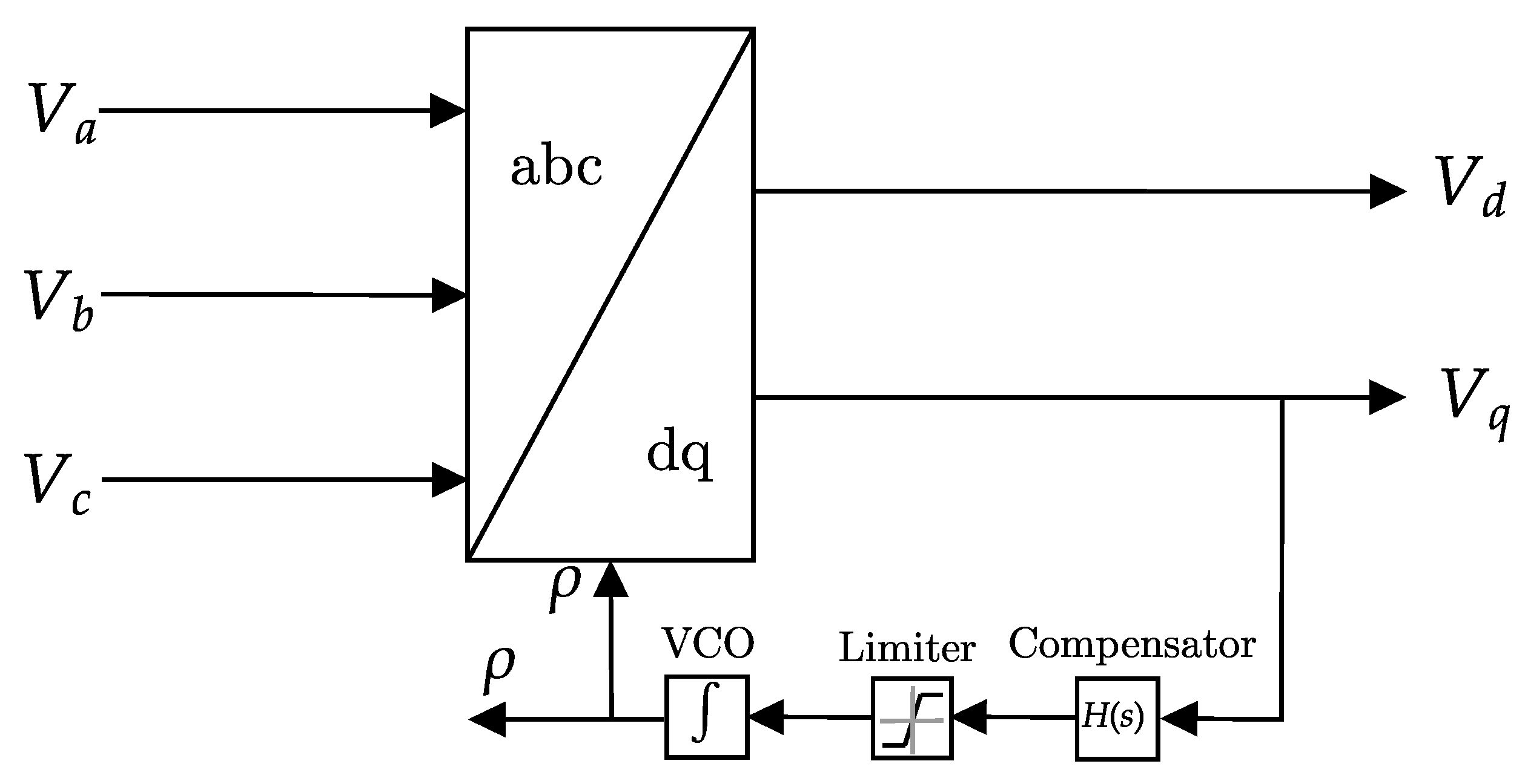
The difference between the input, ${\omega }_{0}t+{\theta }_0$, and the output, $\rho$, is transmitted through the transfer function, $H\left(p\right){\widehat{V}}_s$, to perform the management of this feedback system. The detailed scheme of PLL operation is shown in Figure 3. At the PLL’s termination, a voltage-controlled oscillator (VCO) is set up to reset the measured angle once it hits $2\pi$.

The dynamical performance of the PLL is mostly determined by the design of the compensator $H\left(s\right)$ that is defined as follows:

$$H\left(s\right)=H_1\left(s\right)H_2\left(s\right),$$

(17)

where $H_1\left(s\right)$ handles the system requirements and $H_2\left(s\right)$ considers the stability requirements. The PLL has a single integrator at the origin, which is from the VCO. For that, the constant component of the input signal, ${\theta }_0$, can simply be tracked. However, since the input signal has a ramp component that is ${\omega }_{0}t$, another integrator is required to guarantee that the steady-state error approaches zero. The compensator part $H_1\left(s\right)$ may include this pole among the other system’s design requirements.

To prevent malfunctioning in the control process, the PLL should also take care of the distortion, e.g., harmonics, that are embedded in the grid voltage. Otherwise, the distortion in the grid will be reflected in the converted frame, $dq$. The double harmonic component is a significant cause for concern since it has an inherent large magnitude and a frequency that is the closest to the fundamental frequency. The imbalanced component can also lead to stability problems in the grid. We must consider the imbalanced component in designing the PLL mechanism to avoid the PLL malfunctioning. The effect of the double component distortion can be removed from the PLL when one pair of complex-conjugate zeros located at $\pm j2{\omega }_0$ is added to the compensator. As a result, the loop gain increases. In order to reduce the loop gain magnitude beyond the frequency of $2{\omega }_0$, a double real pole is added at $s=-2{\omega }_0$. To date, the compensator taking into account the nominal value of the grid voltage ${\widehat{V}}_{sn}$ and the gain h becomes

$$H\left(s\right)=\left(\frac{h}{{\widehat{V}}_{sn}}\right)\frac{s^2+{\left(2{\omega }_0\right)}^2}{s{\left(s+2{\omega }_0\right)}^2}{H}_2\left(s\right)$$

(18)

The additional specifications pertaining to operational and stability requirements can be seamlessly integrated into the system’s transfer function, represented by $H_2\left(s\right)$. In the context of this specific case study, we opt to conceptualize $H_2\left(s\right)$ as a lead compensator, a vital control component that possesses the ability to inject additional phase margin into the plant system. The choice of design is strategic, as the lead compensator modifies the phase-frequency characteristics of the system to ensure a greater phase margin, which in turn guarantees a more stable and reliable system performance. The integration of a lead compensator into $H_2\left(s\right)$ thus contributes to fortifying the overall stability of the system. By implementing this configuration, we ensure that the system maintains an ample stability margin in relation to the gain crossover.

This is of paramount importance as it aids in averting system instability that could stem from an increase in gain at the crossover frequency. Thus, this design ensures that the system is capable of operating under varying conditions while preserving its stability, thereby resulting in a more robust and dependable control system. With ${\delta }_m$ representing the added phase margin, the lead compensator $H_2\left(s\right)$ is constructed as follows:

$$H_2\left(s\right)=\left(\frac{s+(p/\alpha )}{s+p}\right),$$

(19)

where

$$\begin{array}{cc}\hfill p& ={\omega }_c\sqrt{\alpha },\hfill \\ \hfill \alpha & =\frac{1+sin{\delta }_m}{1-sin{\delta }_m},\hfill \end{array}$$

(20)

By considering the grid and stability requirements, the compensator becomes

$$H\left(s\right)=\left(\frac{h}{{\widehat{V}}_{sn}}\right)\frac{s^2+{\left(2{\omega }_0\right)}^2}{s{\left(s+2{\omega }_0\right)}^2}\left(\frac{s+(p/\alpha )}{s+p}\right).$$

(21)

3. Differential-Algebraic Equations Modeling

Transfer functions are employed to express the model that was provided. We convert the given model from the s-domain to the time-domain in this section. The transformation methodology is generalizable and can be applied to various dynamical systems. We will analyze each component of the system, and in the end, these components will be assembled to run the system. The grid is already expressed in differential equations as in Equation (6).

3.1. Derivation of PLL DAEs

The methodology for deriving the gain parameter, h, involves assessing it within the context of the loop gain, specifically at the crossover frequency of 200 rad/s. The equation that characterizes the loop gain is set to equal 1, which corresponds to the magnitude at the crossover frequency. By considering ${\widehat{V}}_{sn}=391V$, the gain of $H\left(s\right)$ is $h=2.68\times {10}^5$. Without considering the compensator gain and the stability requirements, i.e., $h{H}_2\left(s\right)=1$, the phase angle of the system loop gain at the gain crossover (${\omega }_c=200$ rad/s) is $-{210}^{\circ }$. To guarantee stability, ${60}^{\circ }$ phase margin is added. This criterion can be met using a lead compensator. As the system needs ${90}^{\circ }$, two identical lead compensators of an angle of ${45}^{\circ }$ are used. Following (19), the applied lead compensator

$$H_2\left(s\right)={\left(\frac{s+83}{s+482}\right)}^2.$$

(22)

Thus, the overall compensator is

$$H\left(s\right)=\frac{685.42\left(s^2+568516\right)\left(s^2+166s+6889\right)}{s\left(s^2+1508s+568516\right)\left(s^2+964s+232324\right)}.$$

(23)

The system’s frequency response, which is illustrated in Figure 4, initially presents a decreasing magnitude with a slope of −40 dB/dec. However, upon reaching the frequency of approximately 200 rad/s, a transition occurs: the slope decelerates to −20 dB/dec. Simultaneously, the phase alters its course, transitioning from −180 degrees to −120 degrees. This 60-degree shift can be attributed to the phase margin of the system, which plays a crucial role in maintaining system stability and performance.

Beyond the crossover frequency, the system gain continues its downward trajectory with an unchanging slope of −40 dB/dec. This consistent decline in gain beyond the crossover frequency highlights the system’s inherent ability to suppress higher-frequency components and maintain stability under a range of operating conditions. The imbalanced component corresponding to the frequency of 754 rad/s is effectively attenuated by the designed PLL, thereby aligning $V_q$ to zero. This effective attenuation underpins the efficacy of the designed PLL, demonstrating its capability to maintain system balance and stability despite the presence of an imbalanced component.

The single s in the denominator represents $\omega$ and as it passes the integrator in the VCO it becomes $\rho$, the $abc-dq$ transformation angle. For normal PLL operation, $\omega$ has to be initialized with the grid frequency. To ease the state–space transformation, this integrator is separated from the rest of $H\left(s\right)$, as follows:

$$\begin{array}{cc}\hfill H\left(s\right)& =\frac{\left(s^2+568516\right)\left(s^2+166s+6889\right)}{\left(s^2+1508s+568516\right)\left(s^2+964s+232324\right)}\times \frac{685.42}{s},\hfill \\ \hfill & =\frac{\left(s^2+568516\right)\left(s^2+166s+6889\right)}{\left(s^2+1508s+568516\right)\left(s^2+964s+232324\right)}\times \frac{685.42}{s},\hfill \\ \hfill & =\frac{s^4+166s^3+575.4\times {10}^3{s}^2+943.73\times {10}^{4}s+3.92\times {10}^9}{s^4+2472s^3+225.45\times {10}^4{s}^2+898.39\times {10}^{5}s+1.32\times {10}^{11}}\times \frac{685.42}{s},\hfill \\ \hfill & =\frac{n_1{s}^4+n_2{s}^3+n_3{s}^2+n_{4}s+n_5}{d_1{s}^4+d_2{s}^3+d_3{s}^2+d_{4}s+d_5}\times \frac{h}{s}.\hfill \end{array}$$

(24)

For simplicity, the numerator components are denoted $n_1\dots n_5$, and the denominator components are denoted $d_1\dots d_5$. The process of the state–space transformation first decomposes the transfer function into several integrators. Then, each integrator represents a state of the system. Figure 5 clarifies the procedure.

The system states are revealed by breaking down the PLL compensator’s transfer function, $H\left(s\right)$. Initializing the angular frequency, $\omega$, is required for PLL operation, as was previously explained. For this model, ${\dot{x}}_5$ represents $\omega$. Given that the system’s frequency is $60 \mathrm{Hz}$, the initialization of ${\dot{x}}_5$ is performed by $60\times 2\pi$ rad/s. Furthermore, to guarantee the normal performance of the PLL, $\omega$ must be constrained so that the transformation angle does not highly deviate from the grid angle. The transformation angle, $\theta$, is represented by the state ${\dot{x}}_6$. For that, the integrator, which is indicated as VCO, resets itself as it reaches $2\pi$. The purpose of the VCO is to achieve physical meaning, which is the circular rotation of the angle. The state–space form of the PLL

$$\begin{array}{cc}\hfill \frac{d}{dt}\left[\begin{array}{c}{x}_1\hfill \\ x_2\hfill \\ x_3\hfill \\ x_4\hfill \\ x_5\hfill \\ x_6\hfill \end{array}\right]=& \left[\begin{array}{cccccc}-d2& -d3& -d4& -d5& 0& 0\\ 1& 0& 0& 0& 0& 0\\ 0& 1& 0& 0& 0& 0\\ 0& 0& 1& 0& 0& 0\\ (n2-d2)& (n3-d3)& (n4-d4)& (n5-d5)& 0& 0\\ 0& 0& 0& 0& h& 0\end{array}\right]\left[\begin{array}{c}{x}_1\hfill \\ x_2\hfill \\ x_3\hfill \\ x_4\hfill \\ x_5\hfill \\ x_6\hfill \end{array}\right]+\left[\begin{array}{c}{V}_q\hfill \\ 0\hfill \\ 0\hfill \\ 0\hfill \\ 0\hfill \\ 0\hfill \end{array}\right],\hfill \\ \hfill {\dot{x}}_5\left(0\right)& ={\omega }_0,\hfill \\ \hfill {\omega }_{min}& \le h\times {\dot{x}}_5\le {\omega }^{max}.\hfill \end{array}$$

(25)

While the model can be run to operate by itself as an individual system, it can be extended to different grid configurations. For both cases, the input is $abc$-frame and the output is the regulated $dq$-frame.

3.2. Derivation Grid-Following Inverter DAEs

To reveal the state of feed-forward and feedback compensators, their transfer functions are expanded, as shown in Figure 6. The states $x_7$ and $x_8$ belong to feed-forward compensators. The states $x_9$ and $x_{10}$ refer to the states of the feedback compensators. The states $x_{11}$ and $x_{12}$ represent the inductor of the grid. The state–space model follows

$$\begin{array}{cc}\hfill \frac{d}{dt}\left[\begin{array}{c}{x}_7\hfill \\ x_8\hfill \\ x_9\hfill \\ x_{10}\hfill \\ x_{11}\hfill \\ x_{12}\hfill \end{array}\right]=& \left[\begin{array}{cccccc}\frac{-1}{g_f}& 0& 0& 0& 0& 0\\ 0& \frac{-1}{g_f}& 0& 0& 0& 0\\ 0& 0& 0& 0& -K_i& 0\\ 0& 0& 1& 0& 0& -K_i\\ \frac{1}{L}& 0& \frac{1}{L}& 0& \frac{-(K_p+R_t)}{L}& 0\\ 0& \frac{1}{L}& 0& \frac{1}{L}& 0& \frac{-(K_p+R_t)}{L}\end{array}\right]\left[\begin{array}{c}{x}_7\hfill \\ x_8\hfill \\ x_9\hfill \\ x_{10}\hfill \\ x_{11}\hfill \\ x_{12}\hfill \end{array}\right]+\left[\begin{array}{c}\frac{V_{sd}}{g_f}\hfill \\ \frac{V_{sq}}{g_f}\hfill \\ K_i{i}_{dref}\hfill \\ K_i{i}_{qref}\hfill \\ \frac{-(V_{sd}-K_p{i}_{dref})}{L}\hfill \\ \frac{-(V_{sq}-K_p{i}_{qref})}{L}\hfill \end{array}\right].\hfill \end{array}$$

(26)

4. Numerical Integration Methods

Dynamical systems that are characterized by differential-algebraic equations can be resolved and simulated through three prominent numerical integration methods: the Forward Euler Method (FEM), the Backward Euler Method (BEM), and the Implicit Trapezoidal Method (ITM). Each of these methods possesses its unique set of advantages and limitations; hence, the choice of an appropriate method should be tailored to align with the specific attributes and requirements of the application at hand. The standard form of the explicit ordinary differential equation is

$$\dot{x}=\left(x,u\right),$$

(27)

where x and u denote the state and the input of the system, respectively. FEM is a first-order technique, and the process of its integration is straightforward. The state step is mainly based on the preceding state step. FEM is generally formulated as follows:

$$x^{(i+1)}=x^{\left(i\right)}+\Delta tf\left(x^{\left(i\right)},u^{\left(i\right)}\right),$$

(28)

where $x^{\left(i\right)}$ is available from the prior step and $\Delta t$ is the time step. Despite its reputation for simplicity and stability, FEM is the least precise method.

BEM is an implicit method and is known for its high stability. BEM integrates the previous state with the current state, which is attained by numerical approaches, such as the Newton method if the system contains nonlinear components. The BEM standard form is

$$x^{(i+1)}=x^{\left(i\right)}+\Delta t\mathit{f}\left(x^{(i+1)},u^{(i+1)}\right).$$

(29)

As previously mentioned, BEM is particularly useful when the system is nonlinear, which is a fundamental property of models of power systems. The following is the implementation of the Newton technique on the BEM. The standard form is set as

$${\mathbf{0}}_{n,1}=x^{\left(i\right)}+\Delta t\mathit{f}\left(x^{(i+1)},u^{(i+1)}\right)-x^{(i+1)},$$

(30)

which is equivalent to

$${\mathbf{0}}_{n,1}=\mathit{h}\left(x^{\left(i\right)},x^{(i+1)},u^{(i+1)},\Delta t\right)={\mathit{h}}^{(i+1)}.$$

(31)

The k-th iteration of the Newton solving process is

$$x_{(k+1)}^{(i+1)}=x_{\left(k\right)}^{(i+1)}-{\mathbf{H}}_{\left(k\right)}^{(i+1)}{\mathit{h}}^{(i+1)},\mathrm{for}k=1,2,\dots ,$$

(32)

where

$${\mathbf{H}}_{\left(k\right)}^{(i+1)}=\frac{\partial {\mathit{h}}^{(i+1)}}{\partial x_{\left(k\right)}^{(i+1)}}=\Delta t\frac{\partial {\mathit{f}}^{(i+1)}}{\partial x_{\left(k\right)}^{(i+1)}}-{\mathbf{I}}_n.$$

(33)

The initial value of the state iteration is $x_{\left(0\right)}^{(i+1)}=x^{\left(i\right)}$.

The implicit Trapezoidal Method (ITM) combines the BEM and the FEM to provide excellent stability and precision in the calculation. The ITM is attained by combining the FEM and BEM as follows:

$${\mathit{h}}^{(i+1)}=x^{\left(i\right)}+\frac{1}{2}\Delta t\mathit{f}\left(x^{\left(i\right)},u^{\left(i\right)}\right)+\frac{1}{2}\Delta t\mathit{f}\left(x^{(i+1)},u^{(i+1)}\right)-x^{(i+1)},$$

(34)

and

$${\mathbf{H}}_{\left(k\right)}^{(i+1)}=\frac{\partial {\mathit{h}}^{(i+1)}}{\partial x_{\left(k\right)}^{(i+1)}}=\frac{1}{2}\Delta t\frac{\partial {\mathit{f}}^{(i+1)}}{\partial x_{\left(k\right)}^{(i+1)}}-{\mathbf{I}}_n.$$

(35)

The ITM is one of the most trustworthy and efficient techniques. In fact, it is the solver of preference for commercial and noncommercial power system software products. The ITM standard form is

$$x^{(i+1)}=x^{\left(i\right)}+\frac{\Delta t}{2}\mathit{f}\left(x^{(i+1)},u^{(i+1)}\right)+\frac{\Delta t}{2}f\left(x^{\left(i\right)},u^{\left(i\right)}\right).$$

(36)

5. Case Study

5.1. Robust PLL Performance under Voltage Imbalance Conditions

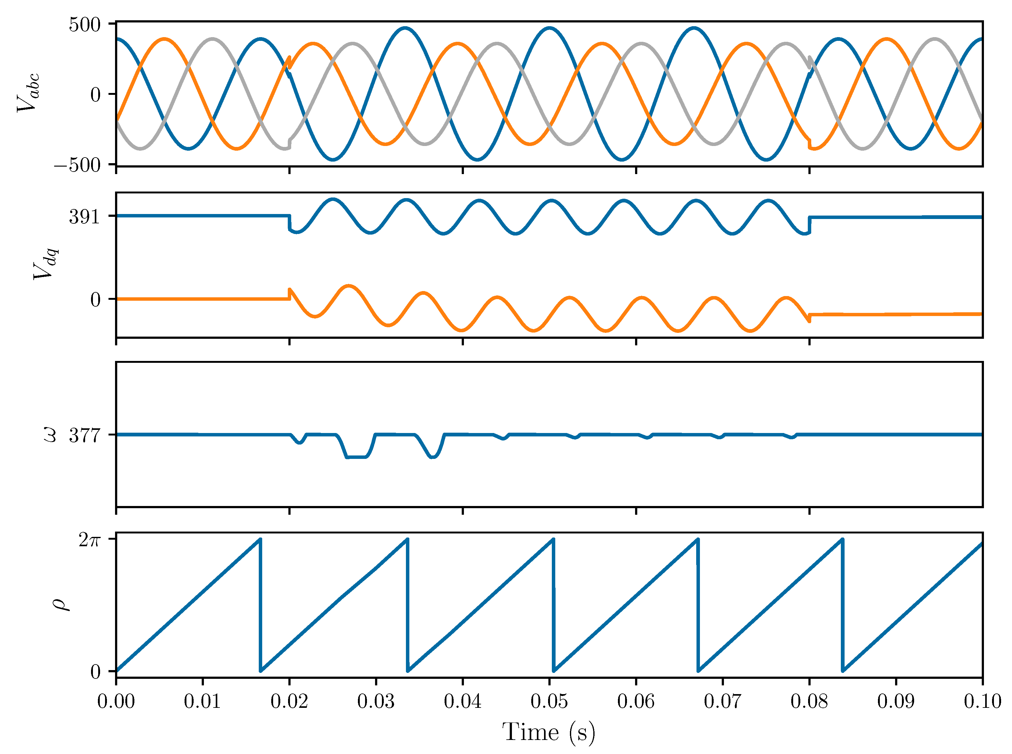
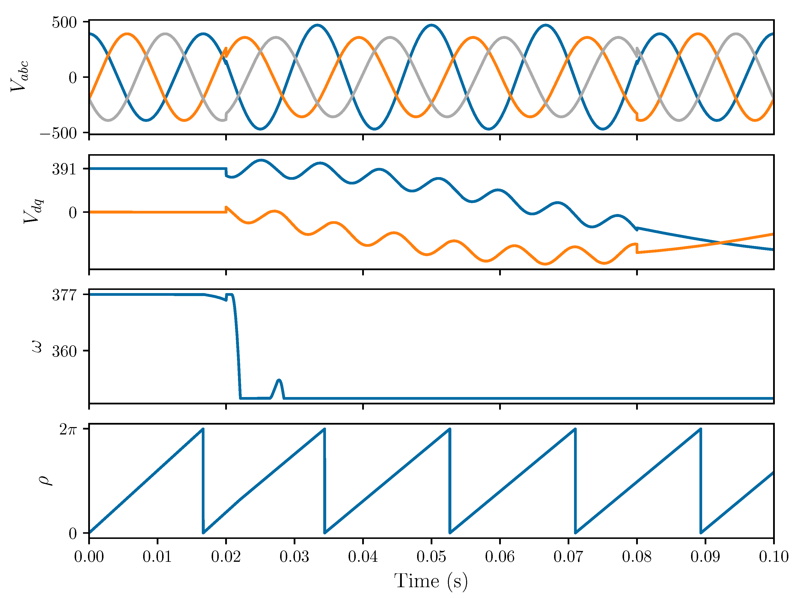
In the design of modern power systems, an essential consideration is the ability to maintain a stable operation in the presence of voltage imbalances. This case study presents a thorough evaluation of the proposed PLL model (26), demonstrating its robust performance under various conditions, including the presence of voltage imbalances. The PLL model, grounded in the natural behavior of the operating system, is specifically designed to address the challenges posed by imbalanced components, a common occurrence in distribution systems. A comprehensive simulation is conducted, assessing the model’s response to three distinct scenarios, as illustrated in Figure 7.

Initially, the PLL operates under ideal conditions, with pure voltage composed solely of the fundamental component. This baseline evaluation serves to validate the model’s performance when no imbalances are present. Following this, at t = 0.02 s, an imbalance is introduced to the system to assess the PLL’s ability to adapt and maintain accurate and stable operation. The simulation results show that the PLL continues to function effectively, with the distortion caused by the imbalance manifesting primarily in the direct- and quadrature-axis voltage components, $V_d$ and $V_q$. This observation confirms the model’s ability to handle voltage imbalances while producing minimal distortion in the output voltages. Finally, at t = 0.08 s, the imbalance is removed from the system, allowing for the evaluation of the PLL’s response to the restoration of balanced conditions. The simulation demonstrates that the PLL promptly returns to smooth operation, reaffirming its adaptability and resilience in the face of varying operating conditions.

The case study under consideration was also subjected to tests involving the ordinary Phase-Locked Loop (PLL) to evaluate its performance and effectiveness under circumstances of imbalanced operational conditions. This meticulous examination was orchestrated to assess the resilience of the PLL when it encounters conditions that veer from the balanced state, thus testing the robustness of its design. The outcomes of the simulation are visually represented in Figure 8. The graphic illustration provides a clear representation of the system’s behavior during and after the intrusion of the imbalanced component. A careful inspection of the figure reveals that the performance of the PLL begins to exhibit signs of deterioration immediately following the onset of the imbalanced component. This indicates that the system’s stability and efficiency are adversely affected by such disruptions.

In the specific context of operations under the influence of the imbalanced component, it is noteworthy that the PLL encounters difficulty in accurately detecting the fundamental frequency of the grid. This is a significant observation as it highlights the limitations of the PLL under non-ideal conditions. Furthermore, it is observed that, once the imbalanced component is eliminated from the system, the PLL is unable to revert to its normal operation. This suggests a lack of adaptive recovery mechanisms in the PLL to restore balance and resume normal functioning after the system experiences instability. This inability to self-correct and re-establish normal operating parameters underscores the need for further improvements in the design and control strategy of the PLL to enhance its resilience to imbalances and other operational anomalies.

5.2. Grid-Following Inverter

In this study, a grid-following Inverter-Based Resource (IBR) is employed to evaluate the effectiveness of the proposed approach. To establish a reliable comparison, parameters from [23] are adopted, as presented in

Table 1. Model parameters.

Parameter	Value
${\omega }_0$	377 rad/s
$V_{s}d$	391 V
L	100 μL
R	0.75 Ω
$r_{on}$	0.88 Ω
$V_{DC}$	1250 V
$f_s$	3420 Hz
$g_f$	$8\times {10}^{-6}$
${\tau }_i$	2 ms
$k_p$	0.05
$k_i$	0.815

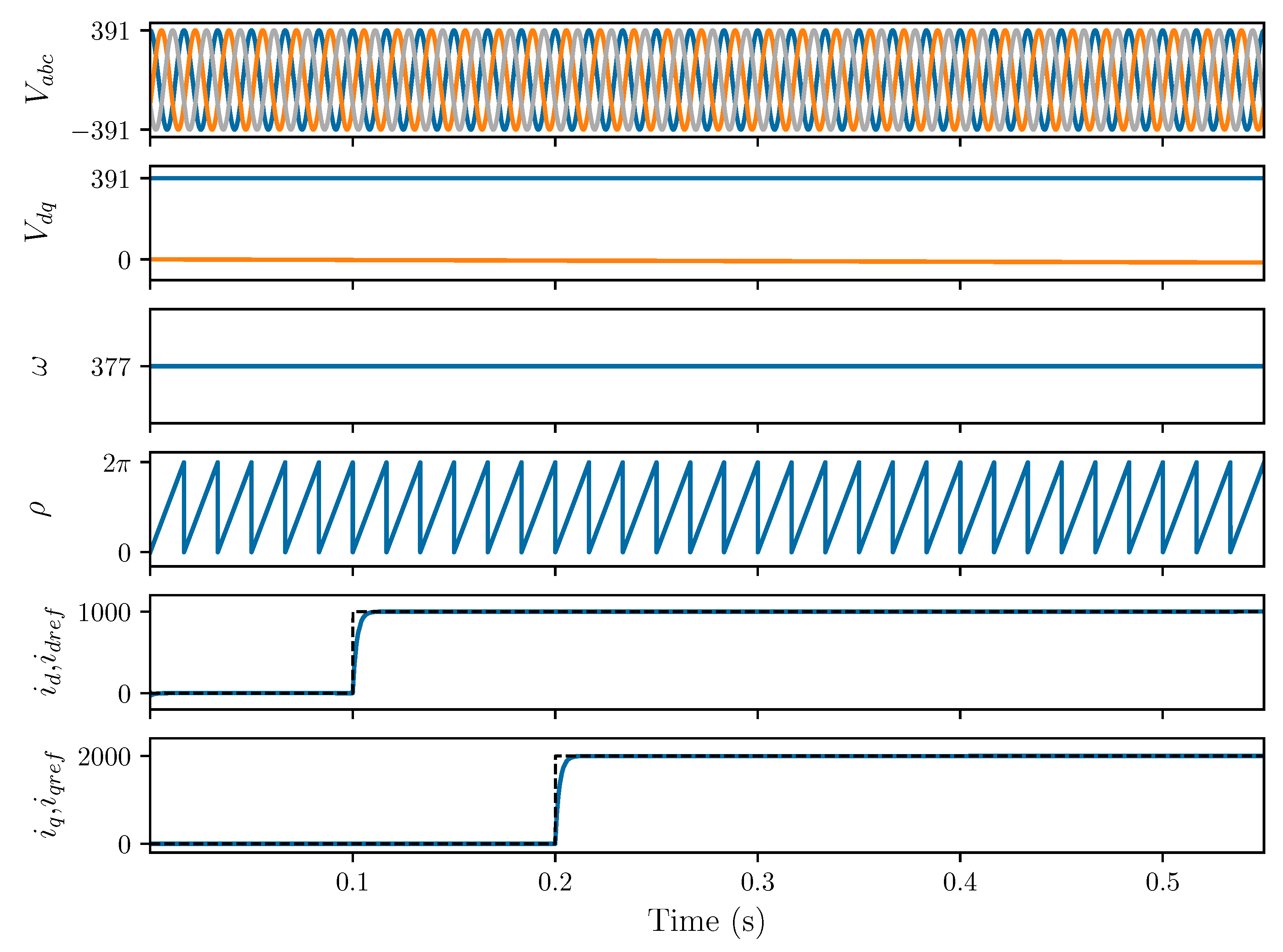
. The system simulation is implemented using the Implicit Trapezoidal Method, a numerical integration technique discussed in a previous section. The Python-coded simulation results are illustrated in Figure 9.

Figure 9 comprises several subplots, each representing various aspects of the inverter’s performance. The first subplot highlights the voltage at the AC side of the inverter, specifically at the Point of Common Coupling (PCC), which connects the inverter to the grid. As expected, during normal operation, the three-phase grid voltage remains balanced. The second subplot depicts the $dq$-frame voltage corresponding to the three-phase grid voltage. The Phase-Locked Loop (PLL) accurately transforms the $abc$-frame to the $dq$-frame, as evidenced by the plot. The simulation of this part is modeled using Equation (25).

The third subplot illustrates the grid angular frequency measured by the PLL. In the state–space model, the angular frequency is denoted by $x_5$. The grid angle, represented by $x_6$, is computed by integrating the limited angular frequency. While regular integrators can perform this integration, resettable integrators are necessary to restrict the angle range between 0 and $2\pi$.

The fifth subplot demonstrates the inverter current aligned to the d-axis and its reference. The active power, as explained in Equation (8), is related to this current and can be primarily regulated using it. To assess the effectiveness of the control applied to $i_d$, the reference current, $i_{dref}$, starts with a value of 0 and is changed to 1000 at t = 0.1 s. As observed in the plot, the response of $i_d$ adequately follows its reference.

Similarly, the sixth subplot shows the inverter current that is aligned to the q-axis and its reference. The reactive power is associated with it, $i_q$, as in Equation (8). Furthermore, its response is tested to validate the system control. The reference current, $i_{qref}$, starts with a value of 0, and is then changed at t = 0.2 s to 2000. As displayed, the response appropriately changes and matches its reference.

5.3. Grid-Following Inverter under Grid Voltage and Frequency Variations

To evaluate the robustness of the system under investigation, we subjected it to a series of stress tests designed to mimic abnormal conditions which may realistically occur in an actual power system. This approach was undertaken with the intent of assessing how well the system could maintain its operational integrity under unexpected circumstances, a critical aspect of real-world system resilience. Among the various adverse conditions considered, we focused on two key events that frequently transpire in power grids: drops in voltage and frequency. These scenarios were carefully incorporated into our case study, the results of which are visually represented in Figure 10.

In the conducted simulation, the inverter initially operates under normal conditions. However, at t = 0.08 s, we introduced a disruption by reducing the grid voltage to 85% of its nominal value. This sudden drop persisted until 0.2 s, at which point we allowed the grid to recover to its nominal voltage. The response of the designed PLL to this sudden change was prompt and effective. The PLL swiftly tracked the alteration in grid voltage and mirrored it in its DC values, thereby demonstrating its ability to respond to voltage variations. As depicted in Figure 10, the PLL was also capable of restoring normal operation in sync with the grid recovery, further illustrating its adaptability and resilience.

Next, at t = 0.3 s, we implemented another disruption by altering the grid frequency from its standard 60 Hz to 59.95 Hz. This frequency variation lasted for a brief duration of 0.01 s. The impact of this frequency change was observable in the PLL output, primarily affecting the $V_q$ component. Despite these disturbances, the PLL demonstrated its robustness by swiftly regaining its normal state after a recovery period of 0.2 s. This rapid recovery underscores the PLL’s ability to maintain system stability and performance even under challenging conditions, thus confirming its efficacy and robustness in the face of real-world grid disturbances.

6. Conclusions

The penetration of IBRs that interface renewables and DERs changes the power system infrastructure. The importance of modeling can never be overstated. Transfer functions are frequently used to model the grid connection of IBRs. On the other hand, this paper models it with differential-algebraic equations which can be converted into state–space form. The state–space modeling is superior to the transfer function modeling in addition to being in the time domain. Multiple-input, multiple-output systems, and time-variant systems can both be handled by the state–space approach. State–space models can also be employed to implement Kalman filters. We also develop the state–space model of a PLL customized to address imbalanced components. Reaching improved methods of analysis and simulation is the purpose of achieving a different sort of modeling. Furthermore, preparing the system for the deployment of state–space optimal control strategies is another objective of the grid-following IBR state–space model development. By employing primary integration methods capable of addressing nonlinear systems, our proposed model has been numerically solved, demonstrating a precise correspondence between the transfer function model and the state–space model. Through the case studies presented, the validity and robustness of the state–space approach have been further substantiated, providing a strong foundation for future research and development in the field of power electronics and grid integration.