A Discrete Cooperative Control Method for Production Scheduling Problem of Assembly Manufacturing System

Abstract

With a sharp decrease in resource utilization of the complex production process, integrated scheduling methods are urgently needed in assembly manufacturing industries. To this end, this paper presents an integrated scheduling with jobs processing and assembly sequence (ISJPAS) problem where jobs and assemblies can be processed simultaneously. As the first contribution to this work, we develop a mixed integer nonlinear programming model (MINLP) that aims at minimizing maximum completion time and determining the earliness and tardiness of jobs and resulting inventory time. The structured property of the optimal scheduling solution is analyzed with regard to job sequencing and assembly sequencing. The NP-hard nature of the problem is proved, which provides upper and lower bounds on the optimal solution. Second, an efficient discrete assembly time and arrival time control (DAATC) method is presented based on continuous time variable control models. From a modified set of benchmark problems, the proposed method is tested by comparing four assembly association levels in real applications. The comparisons indicate the potentiality of our method to satisfy the due date. Lastly, relevance of practical applications are discussed, and several future research avenues are emphasized.

1. Introduction

The manufacturing industry is the foundation of a national economy, where its rise or fall is directly related to national competitiveness and national security. Influenced by the integration of the global economy and market diversification, the demand for products in society has gradually shifted to personalization, diversity, and dynamic variability, resulting in an increase in the variety of products, a reduction in batch sizes, and a significantly shorter life cycle. Discrete factories are physical entities that engage in the production and processing of parts and components of mechanical products. It is also the earliest manufacturing environment to be exposed to a wide range of variables [1]. In particular, an assembly manufacturing system is an integrated discrete production system where various manufacturing operations are simultaneously and independently processed, then the jobs are collected and transported to assembly lines arranged in the assembly shop for “factory assembly operations”. Specifically, the production process is divided into two stages, namely, processing and assembly, which require a production schedule to include these two disjoint stages [2]. It is called the integrated scheduling with jobs processing and assembly sequence (ISJPAS) problem [3]. Since the shared production resources are limited, multiple products cannot be processed simultaneously. The different processing times and process paths of each job also lead to the existence of assembly associated jobs in significant scheduling collaboration difficulties. Hence, it is necessary to investigate further the interplay between production scheduling and assembly sequence planning.

ISJPAS problem, which belongs to the non-deterministic polynomial hard (NP-hard) problem, is a complex hierarchical coupling constrained (HCC) optimization problem that offers robust perturbations. In recent years, researchers have spent quite a considerable effort on ISJPAS. One of the earliest works was from Sculli [4], in which he built a dynamic JSP with the assembly process and adopted the priority scheduling rules that contained dynamic information of jobs to optimize Makespan. Prior research on the performance of the ISJPAS problem has primarily focused on scheduling models, intelligent algorithms, and objective functions [5]. In contrast, research on its coupling and synergistic operation mechanism is relatively sparse. This paper intends to explain the coupling constraints between the production shop and the assembly shop and to contribute to the further development of such assembly manufacturing systems.

Production scheduling is defined as determining the times of controlled events on the manufacturing shop floors. Note that the scheduling problem corresponds to the system that comprises discrete-time processes. Modeling is a precondition for manufacturing system simulation. Modeling methods such as discrete event simulation, system dynamics, and Petri nets cannot directly analyze the dynamic coupling characteristics in assembly manufacturing systems [6,7,8]. For example, reduced variance in job completion times is an important factor in just-in-time production because it simultaneously reduces process inventory and delays. However, feedback control theory modeling is a powerful tool that deals with the coupling mechanism of production scheduling problems. Since the first attempts by Prabhu and Duffie [9], feedback control theory has been applied to various production–inventory problems and work in process control problems [10]. It is used as a mechanism to compensate for global information by which job entities iteratively adjust the time required by the machine.

On the whole, the contributions of this paper lie in the detailed analysis of the discrete cooperative control model for the assembly manufacturing system. To this end, we first analyze the parallel production module of the assembly manufacturing system, which is a part of production schedules and can effectively lower the overall inventory cost level. In particular, a mathematical model of the flexible assembly job shop scheduling problem is developed and its solution NP-hard proof and upper and lower bounds are discussed. Furthermore, to overcome the large computational burdens that are expected from the non-linearity of the objective function, a discrete cooperative control method based on distributed assembly time and arrival time control (DAATC) is represented. This control model as the central control logic of dynamic algorithms is designed for real-time production and cooperative scheduling, thereby simultaneously realizing better makespan as well as tardiness costs.

The remainder of this paper is structured as follows: Section 2 reviews related work in flexible assemble job shop scheduling problem and control theory for production scheduling. The parallel production module and mathematical models for the assembly manufacturing system are proposed in Section 3. Specifically, this section proves the strongly NP-hard problem of the FAJS as well as discusses the upper and lower bounds of the optimal solution. Then, the discrete cooperative control methods based on distributed arrival time control are represented in Section 4. Section 5 provides the computational results and the discussions. Lastly, the conclusions of this research are summarized in Section 6.

2. Related Works

Considerable literature could be found about the relevant topics of this study. We limited our review to the literature published in the last two decades and focused on the problem dimensions and control theory methodology.

2.1. Integrated Scheduling with Jobs Processing and Assembly Sequence Planning

Customized orders bring new challenges and problems for processing and production activities: (1). The instability of the production process creates a high unevenness in the temporal and spatial dimensions of the production load on the shop floor. First of all, in terms of time dimension, the business demand for customized assembly products is unstable, and when the market demand is high, the workshop runs at full capacity to meet the production needs. In the spatial dimension, the demand for the same type of processing resources may be more concentrated in a certain period of time, as the processing paths and working time requirements of different tasks are quite different. (2). Associated parts with assembly constraints make production schedule coordination more difficult. The parts under the assembled products need to be processed in the machining shop first, and then enter the assembly shop at the same time as far as possible according to the demand of the assembly material set to reduce the waiting time for the assembly of the products [10].

In the above background, focusing on the current research status of the ISJPAS problem, we review and discuss three aspects of the ISJPAS problem, namely, the integrated process planning and scheduling (IPPS) problem, the assembly job shop scheduling (AJSS) problem, and the ISJPAS problem.

Chu et al. [11] constructed a two-level planning model oriented to product uncertainty in IPPS. It describes the upper-level process planning model with a mixed integer planning method and handles the lower-level shop floor scheduling problem with an agent-based modeling method. Rietz et al. [12] developed a pseudo-polynomial network flow model that integrates medium-term process planning and short-term shop floor scheduling. For multi-product single-stage batch plants with parallel cells and resource constraints, combined with manufacturing service concepts, Aguirre and Papageorgiou [13] presented a novel model for the integration of IPPS with machine maintenance and repair. The above studies show that the integrated model built by the IPPS pays attention to the hierarchical relevance of process planning and job shop scheduling. Fattahi et al. [14], employing a hybrid algorithm, proposed a mathematical model where the objective is to minimize the completion time of all products for flexible shop scheduling with assembly operations. In this model, the jobs need multiple operations to be processed on each machine in the flexible shop and multiple jobs to be assembled on the assembly machine. In the first stage, jobs are machined in the flexible shop; the job is assembled on the assembly machine in the second stage. Zheng et al. [15] employed an improved master-disciple evolutionary algorithm to solve the AJSS problem with maximum completion time and stability. The operation sequence is constrained by the extended adjacency matrix of the subassemblies.

At present, the research on production scheduling is mainly focused on the flexible job shop scheduling problem (FJSP), rarely integrating the machining process and assembly operation [16]. Nourali and Imanipour [17] first introduced the assembly job scheduling problem with sequence-dependent setup times coined as the flexible job shop scheduling problem (FAJSP). A mixed integer linear programming (MILP) model was proposed to address this problem, which can be solved with good results in small instances. Subsequently, they [18] proposed a particle swarm optimization algorithm to solve large-sized FAJSP. The results are comparable to branch and bound and much less time efficient. Inversely, both studies handled static scheduling environment problems. Zhang et al. [19] proposed a constraint rule (CP) model that was built with three models (constraint programming model, mixed integer programming model, and scheduling rule) to minimize makespan for FAJSP in a dynamic scheduling environment. Later, they [20] deeply investigated distributed particle swarm optimization to solve multi-objective optimization problems (makespan, total tardiness, and total workload). Lin et al. [21] treated machining and assembly as a class of jobs and joined the job’s tight constraints relationship. And multi-objective genetic algorithm with heuristic rules was provided to optimize three objective scheduling problems (makespan, total energy consumption, and the number of machine turn-off/on). Zheng et al. [22] applied the master-apprentice evolutionary algorithm to cope with the assembly job-shop scheduling problem with random machine breakdown and uncertain processing time.

2.2. Control Theoretic Model for Production Scheduling

Scheduling problems are a combination in nature, which are difficult to solve. Generally, three methods have been studied to solve these difficult problems: (1) classical operations research, (2) simulation, and (3) control theory. Prabhu and Duffie [23] first developed a continuous-variable feedback control system to predict the part arrival time trajectories and derive the steady-state value closed-form expression using nonlinear differential equations and Filippov for the heterarchical manufacturing scheduling systems. This method, called the real-time distributed arrival time control system (DATC), transforms the combinatorial scheduling problem into a dynamical problem of continuous variable control. Cho and Lazaro [24] studied the unified control system that integrated distributed production scheduling and CNC-level machine capacity control using a continuous control theory method for the shop floor. Later in Cho and Prabhu [25], a new double integral arrival time controller (DIAC) was proposed to solve the predictable production scheduling model. Grundstein, Freitag, and Reiter [26] proposed an autonomous production control (APC) method that addresses three control tasks (order release, sequencing, and capacity control). Chen and Wang [27] analyzed the approximate optimal production control strategy to evaluate the average production cost of the multi-stage assembly system. Xu and Lei [28] presented a feedback control method to address the production scheduling problem that considers makespan and energy consumption in a rolling horizon framework. Duffuaa et al. [29] introduced a novel model that integrated and optimized production scheduling, inventory holding, maintenance, and process control decisions simultaneously for a single machine.

From the review of relevant research, it is observed that there is currently some research on the integrated scheduling of processing operations and assembly sequence, but it is not considered that the product assembly sequence and assembly constraints affect the total production completion time and part inventory time during the production process. On the one hand, the inventory time of each job is affected by the assembly sequence in the processing and assembly of the parallel job. On the other hand, the assembly times are impacted by the processing sequence of jobs scheduled on the shop floor. It is necessary to further investigate the interaction between job shop scheduling and assembly sequence planning that considers the relationship between the job processing process and the assembly process. A discrete cooperative control method integrating job shop scheduling and assembly sequence planning is proposed to improve production efficiency and save manufacturing costs.

3. Problem Definition and Model Construction

This section provides more information about the integration model. Section 3.1 summarizes a novel parallel production module in a discrete manufacturing shop. In Section 3.2, the mathematical model of the flexible assembly job-shop scheduling problem is proposed. Section 3.3 discusses its solution NP-hard proof and upper and lower bounds are discussed.

3.1. Parallel Production Module in Assembly Manufacturing System

The assembly manufacturing process of complex and large products usually consists of job processing procedures and product assembly procedures. Among them, there are two main production modules: the traditional production module and the parallel production module [30].

The traditional production module provides shop floor scheduling and assembly sequence planning, respectively, as shown in Figure 1a. This way can only start the assembly process after all jobs have been finished, which leads to a longer total production completion time. Furthermore, job processing time can be minimized through shop floor scheduling, as well as assembly time can be reduced through assembly sequence planning. Nonetheless, this way usually results in a long inventory time before the jobs are assembled into the final product, as shown for jobs i and j in Figure 1a.

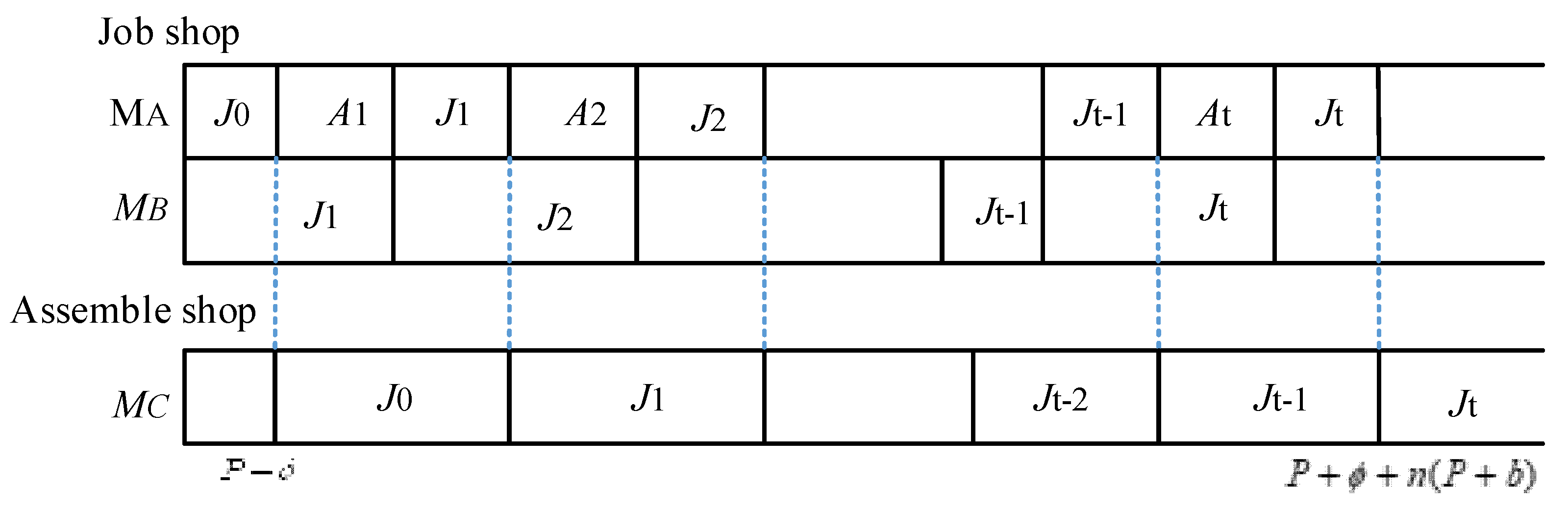
To overcome the above problem, the parallel production module performs the part machining process and the assembly process simultaneously, as shown in Figure 1b. Once the jobs that need to be assembled are machined, the job assembly can begin. However, early completion of jobs results in inventory occupancy before the part is assembled into the product; conversely, late completion of jobs results in longer wait times before the part is assembled into the product. The improved parallel production module eliminates the assembly wait time by varying the processing sequence and assembly sequence of the jobs, as shown in Figure 1c.

The above analysis shows that the inventory time of each job is affected by the assembly sequence; on the other hand, the assembly time is influenced by the job processing sequence generated by shop scheduling. Hence, it is necessary to study the synergistic operation mechanism of the part machining process and the assembly process, and then propose a feedback control method. The method obtains an integrated optimal production sequence that includes the part machining sequence and the assembly sequence, which also allows for minimizing the waiting time of the jobs during the assembly process.

3.2. Mathematical Model

The three-parameter method $\alpha \left|\beta \right|\gamma$ was proposed by Graham et al. [31] to describe the scheduling problem. Here, $\alpha$ denotes the machine processing environment, $\beta$ represents the job processing characteristics, and $\gamma$ indicates the description of the processing performance index. In 2012, Nourali and Imanipour [17] first proposed the flexible assembly job shop scheduling problem, and then, it has been studied by more and more scholars. According to an expository paper on assembly scheduling published by WU et al. [32], we define the flexible assembly job shop scheduling problem can be defined as the $F_2(J_{m1},J_{m2})\left|\right|C_{\max }$ problem. Among them, $F_2$ is the processing plans stage production layout. $J_{m1}$ shows the processing stage production layout. $J_{m2}$ represents the assembly stage layout. $C_{\max }$ defines the optimization objectives.

Integrated scheduling with jobs processing and assembly sequence problem: There is a product processed on the $m$ machine. The product is composed of $n$ jobs with assembly constraints. Each job has multiple process paths. Each job needs to be processed in one or more operations, and each operation can be processed by any machine from a given set of available machines $m$, which are assembled after machining. A higher-level subassembly or final product is formed by alternatives from the set of assembly machines $A$. The constraint occurs when there are assembly relationships between jobs. During the assembly of the product, the same product has a different assembly sequence. Determining the process route of each job and selecting the machine tool, machining sequence, and the start time of each operation enables the optimization index. The following assumptions and constraints are considered.

(1)

The processing times of each operation by each machine are determined and known.

(2)

One operation can only be processed by one machine at a time.

(3)

The sum of the start time and processing time of an operation is less than or equal to the makespan of the operation.

(4)

Makespan of the previous operation is less than or equal to the start time of the next operation.

(5)

All jobs can be machined at zero moments.

(6)

Completion time of products is the sum of processing time and assembly time.

(7)

Operation cannot be interrupted during the machining process.

(8)

Operation of each machine is cyclic.

(9)

The transportation time and waiting time of the material are omitted.

The indices and parameters used in this model are summarized in

Table 1. Indices and parameters used in the model.

Sets	Description	Indices	Description
$I$	Set of products	$i$$, i\prime$	Indices of the product
$J_i$	Set of the $i-th$ jobs	$j$$, j\prime$	Indices of the job
$P_{ij}$	$\mathrm{Set} \mathrm{of} \mathrm{the} i-th$ process path	$l$	$\mathrm{Indices} \mathrm{of} \mathrm{the} \mathrm{process} \mathrm{path}, p\in P_{ij}$
$M_{ij}$	$\mathrm{Set} \mathrm{of} \mathrm{the} i-th$ machines	$m$	$\mathrm{Indices} \mathrm{of} \mathrm{the} \mathrm{machine}, m\in M_{ij}$
$O_{ijp}$	$\mathrm{Set} \mathrm{of} \mathrm{the} p_{ij}-th$ operation	$k$	$\mathrm{Indices} \mathrm{of} \mathrm{the} \mathrm{operation}, k\in O_{ijp}$
Job-related parameters	Description
$a{t}_i$	Arrival time of products $i$
$d_i$	Delivery time of products $i$
$ap{t}_i$	Assembly time of the products $i$
$o_{ijpf}$	$\mathrm{The} \mathrm{first} \mathrm{operation} \mathrm{of} \mathrm{the} \mathrm{process} \mathrm{path} p_{ij}$
$o_{ijpl}$	$\mathrm{The} \mathrm{last} \mathrm{operation} \mathrm{of} \mathrm{the} \mathrm{process} \mathrm{path} p_{ij}$
$p{t}_{ijpkm}$	$\mathrm{Processing} \mathrm{time} \mathrm{of} \mathrm{processing} \mathrm{equipment} \mathrm{m} \mathrm{used} \mathrm{in} \mathrm{the} \mathrm{operation} k_{ijp}$
$S_{ijpkm}$	$\mathrm{Start} \mathrm{time} \mathrm{of} \mathrm{processing} \mathrm{equipment} \mathrm{m} \mathrm{used} \mathrm{in} \mathrm{the} \mathrm{operation} k_{ijp}$
$C_{ijpkm}$	$\mathrm{Makespan} \mathrm{of} \mathrm{processing} \mathrm{equipment} \mathrm{m} \mathrm{used} \mathrm{in} \mathrm{the} \mathrm{operation} k_{ijp}$
$C_{ij}$	$\mathrm{Makespan} \mathrm{of} \mathrm{the} \mathrm{job} ij$ (makespan of the last operation)
$L$	Extreme value

.

Decision variables:

$$X_{ijp}=\left\{\begin{array}{c}1,if the job choose the process path p\\ 0,\hspace{1em}otherwise\end{array}\right.$$

$$X_{ijpkm}=\left\{\begin{array}{c}1, if the operation k is processed the machine m\\ 0,\hspace{1em}otherwise\end{array}\right.$$

$$Y_{ijpki\prime j\prime p\prime k\prime m}=\left\{\begin{array}{c}1, if the operation k is processed earlier than the operation k\prime on the machine m\\ 0,\hspace{1em}otherwise\end{array}\right.$$

Constraints:

$$C_{ijpk}\le S_{ijp(k+1)}$$

(1)

$$S_{ijpk}+p{t}_{ijpk}\le C_{ijpk}+L(1-X_{ijpkm})$$

(2)

$${\sum }_{pij}{X}_{ijp}=1$$

(3)

$${\sum }_{M_i{}_{jk}}{X}_{ijpkm}=1$$

(4)

$$S_{ijpkm}+p{t}_{ijpkm}\le S{\prime }_{i\prime j\prime p\prime k\prime m}+L(1-Y_{ijpki\prime j\prime p\prime k\prime m})$$

(5)

$${\sum }_{j=1}{\sum }_{k=1}^{o_{ij}}{Y}_{ijki\prime j\prime k\prime m}=x_{ikl}$$

(6)

$${\sum }_{p\in P_{ij}}{\sum }_{k\in M_{ij}}{C}_{ijp{o}_{ipl(i,p)}k}+ap{t}_i\le C_i$$

(7)

where Equation (1) shows that the completion time of the operation is less than or equal to the start time of the next operation. Equation (2) indicates that the completion time of the operation is larger than or equal to the start time of the operation. Equations (3) and (4) represent that the job is processed by only one process path, and only one machine can be selected for each operation. Equation (5) means that the start time of the operation on the equipment is less than or equal to the completion time, and the completion time of the process is larger than or equal to the start time of the process. Equation (6) ensures that the parts with the same machine cannot be processed at the same time. Equation (7) defines order completion time as the completed time of the last job plus assembly time.

According to the literature reviewed [33], makespan is the most sufficiently studied objective. In this study, the objective of the model is as follows:

$$\min F_C=\min C_{\max }=\min (\underset{1\le j\le n}{\overset{\max }{C_j}})=\min ({\sum }_1^n{x}_{jkm}{t}_{jkm})$$

(8)

3.3. Complexity Analysis of the ISJPAS Problem

In this section, the flexible assembly job shop scheduling problem is discussed, which is one of the most highly complex combinatorial optimization problems, and is an extension of the classical job shop problem that performs operations to be scheduled in a set of parallel machines [34]. The jobs need to process two stages, where the first stage is composed of $m_1$ job shop machines and the second stage is composed of $m_2$ assembly machines (parallel machines). Hence, this sequencing problem is equal to the $F_2(J_{m1},J_{m2})\left|\right|C_{\max }$ problem. As previously mentioned, Garey et al. [35] showed that $J_2\left|\right|C_{\max }$ was strongly NP-hard.

The formal description of this problem is specified as follows. The jobs set that contains $n$ jobs are $N=\left\{J_1,\dots ,J_n\right\}$. Each job $J_i$ is composed of $s$ operations $\left\{O_{i1},\dots ,O_{is}\right\}$. With this process sequence on the machine $M_1$, its processing time is $\left\{p_{i1},\dots ,p_{is}\right\}$, respectively. Once the process $O_{ij}$ is started on the machine $M_j$, it cannot be interrupted. The operation $O_{ij}$ can be processed by only one machine at a time. One machine can only be processed for one operation at a time. If and only if the job $J_i$ is completed on the machine $M_1$(denoted by machines $M_A$ and $M_B$) before it can be machined in the second stage on the machine $M_2$. The objective of this problem is to minimize the maximum completion time.

3.3.1. Strongly NP-Hard Proof for the $F_2(J_2,J_1)\left|\right|C_{\max }$ Problem

This combinatorial optimization problem is at least as hard as the job shop problem because the $F_2(J_2,J_1)\left|\right|C_{\max }$ are special cases of combinatorial problems. In the first stage, it is processed on two machines’ job shops (denoted by machines $M_A$ and $M_B$) and then is processed on a single machine (denoted by the machine $M_C$) in the second stage. Let $a_j$, $b_j$, and $c_j$ are processing times of the job $J_i$ ($J_i\in N$) on machines $M_A$, $M_B$, and $M_C$, respectively. It is also known that $J_2|op\le 3|C_{\max }$ and $J_3|op\le 2|C_{\max }$ is proved to be a strongly NP-hard problem [36,37]. Additionally, Williamson et al. [38] proved that it is NP-hard, and $J\left|\right|C_{\max }$ cannot be approximated within 5/4 (unless P = NP).

We now prove that the $F_2(J_2,J_1)\left|\right|C_{\max }$ problem is strongly NP-hard through a reduction of the three-partition problem (Theorem 1). Among them, Johnson [39] concluded the three-partition problem was strongly NP-complete.

Theorem 1.

The $F_2(J_2,J_1)\left|\right|C_{\max }$ problem is strongly NP-hard.

Definition 1.

Three-partition problem (3PP): Given $3t$ integers, $A=\left\{a_1,a_2,\dots ,a_{3t}\right\}$ and an integer$b$. For each element, $j\in A$ there is a positive integer $a_j$ that satisfies $b/4<a_j<b/2$ and ${\sum }_{j=1}^{3t}{a}_j=tb$. The question asks whether there exists a division $A_i$, $(i=1,2,\dots ,t)$ of the set $A$, where each $A_i$ contains three elements of $A$ and  ${\sum }_{j\in A_i}{a}_j=b$,  ($i=1,2,\dots ,t$).

Proof. 

Given an example of a 3PP, we construe the scheduling instance as below.

(1) Number of jobs: $n=4t+1$, $J_i\in \left\{J_0,J_1,\dots ,J_{4t}\right\}$.

(2) Parameters of jobs (processing times of $M_A$, $M_B$, and $M_C$):

$a_0=P+\phi$, $b_0=0$, $c_0=P+b$;

$a_j=P+\phi$, $b_0=P+b$, $c_0=P+b$, for $j\in \left\{1,2,\dots ,t-1\right\}$;

$a_t=P+\phi$, $b_t=P+\phi$, $c_t=0$;

$a_{t+j}=a_j$, $b_{t+j}=0$, $c_{t+j}=0$, for $j\in \left\{1,2,\dots ,3t\right\}$.

(3) Threshold of the objective function is $y=p(t+1)+tb+\phi$.

The above construction can be completed in polynomial time as shown in Figure 2. We further indicate that $C_{\max }^{\ast }$ is no more than $y$ in the schedule when and only when the 3PP instance has one solution. Where $P$ is a positive integer and $\phi$ is an extremely small value ($0<\phi <b/4$). □

3.3.2. Upper and Lower Bounds of the Optimal Solution

In this subsection, the lower and upper bounds of the optimal solution $C_{max}^{*}$ are provided. We first ignore the job scheduling on the machine $M_C$, where the original problem is equated to the two-machine job shop scheduling problem. To solve the optimal solution of the $J_2\left|\right|C_{max}$ problem, we divide the jobs set $N$ into two subsets ($J_1=\left\{J_i\right|p_{i1}<p_{i2}\}$ and $J_2=\left\{J_i\right|p_{i1}\ge p_{i2}\}$). The optimal scheduling is then determined employing James’s algorithm [40] within the polynomial time complexity $O\left(n{m}^2{P}^{4m+1}\right)$. The maximum completion time is denoted as $Q=\mathrm{m}\mathrm{a}\mathrm{x}\{p_{r1}+p_{r2},{\sum }_{i=1}^n{p}_{r1},{\sum }_{i=1}^n{p}_{r2}\}$ where $r={argmax}_i\{\max \left\{a_i|J_i\in J_1\right\}, \mathrm{m}\mathrm{a}\mathrm{x}\{b_i|J_i\in J_2\}\}$. The upper and lower bounds of the optimal solution $C_{max}^{*}$ for this problem are provided by Lemma 1.

Lemma 1.

For the $F_2(J_2,P_1)\left|\right|C_{\max }$ problem, the following lower and upper bounds of the optimal solution $C_{\max }^{\ast }$.

$$\max \{Q+\underset{J_i\in N}{\min }{p}_{i3},\underset{J_i\in N}{\min }(p_{i1}+p_{i2})+{\sum }_{J_i\in N}{p}_{i3}\}\le C_{\max }^{\ast }\le Q+{\sum }_{J_i\in N}{p}_{i3}$$

(9)

Proof. 

(1) The lower bound of the optimal solution for this problem.

When the workshop environment is the $F_2(J_2,P_1)$, three operations of any given job need to be processed on three machines without overlapping. The third operation can only be started when and only when the first two are completed. Hence, the satisfied condition is as follows: $C_{max}^{*}\le \max \left\{Q+\underset{J_i\in N}{\min }{p}_{i3},\underset{J_i\in N}{\min }{(p}_{i1}+p_{i2})+\sum _{J_i\in N}{p}_{i3}\right\}$.

(2) The upper bound of the optimal solution for this problem.

To prove the upper bound on the optimal solution, we construct a feasible schedule. According to the algorithm of Gonzales and Sahni [41], the operations that need to be processed on the machine $M_A$ and $M_B$ are sequenced from the moment 0 until all operations are completed. It is known that the maximum completion time of the job on the machine $M_A$ and $M_B$ is Q. Starting from the moment Q, the operation $O_{i3}(J_i\in N)$ are sequentially processed on the machine $M_C$ until all operations are completed. Obviously, the maximum completion time for feasible scheduling is $Q+{\sum }_{J_{i\in N}}{p}_{i3}$. □

In the next section, the discrete cooperative control model and algorithm are explained as a heuristic method to solve the ISJPAS problem.

4. Discrete Assembly Time and Arrival Time Control Algorithm for Solving ISJPAS

A key issue in handling discrete events in production scheduling is the ability to maintain system performance levels through rapid decision-making. Although significant efforts have been made to develop algorithms that optimize combinations of temporal decisions, these systems are incapable of explaining the influence relationships among themselves because of the combinatorial complexity inherent in them. In this section, we present the dynamic model for the discrete assembly time and arrival time control (DAATC) algorithm. It is based on the integral controller of the real-time distributed arrival time control (DATC) systems [42,43,44], which translates the combinatorial scheduling problem that handles the discrete events manufacturing shops into a feedback control problem with continuous variables in the vector space. 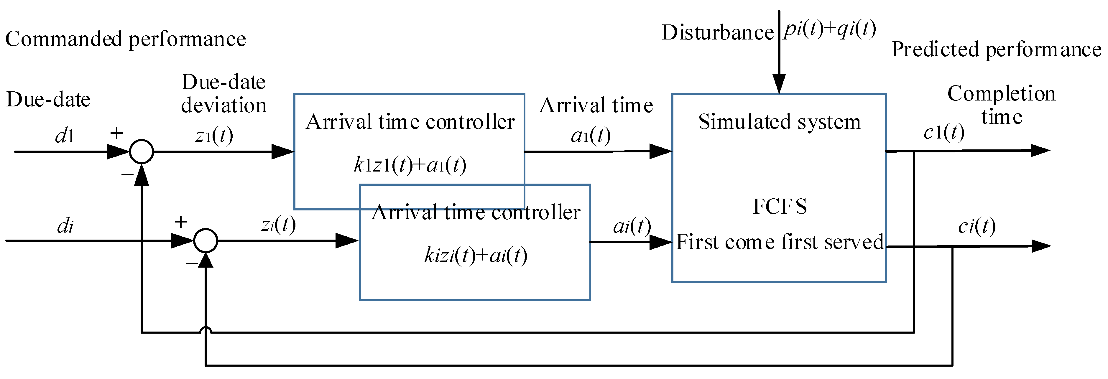Figure 3 indicates the real-time closed-loop control model structure of the DATC systems in discrete time.

The closed loop arrival time controller can be structured for each job entity, where the tentative arrival time is adjusted repeatedly to enhance system performance. For a multivariable closed-loop feedback control system, the adjustments to the arrival time of a single machine can be presented as functions of the continuous time as follows [45].

$$a_i(t)=k_i {\int }_0^t[d_i-c_i(u)]du+a_i(0)$$

(10)

where $k_i$ is control gain. $t$ denotes the discrete time or iteration. And $i$ is the number of jobs. $d_i$, $c_i\left(t\right)$, and $a_i\left(t\right)$ are the due date, completion time, and arrival time of the i-th job, respectively. The first rank derivative of Equation (10) is given below:

$$\stackrel{·}{a_i}(t)=k_i[d_i-c_i(t)]=k_i[d_i-(a_i+q_i+p_i)]$$

(11)

where $q_i\left(t\right)$ is the queuing time when processing starts. It is varied discontinuously according to the different job processing sequences that are defined by the relative sequence of arrival times. $p_i$ is the processing time of the i-th job. Note that the completion time of the jobs is determined by the arrival time, the sequencing time, and the processing time. Equation (10) can be reformulated in the discrete-time domain as below.

$$a_i(mT)=a_i(m-1)T+k_i{z}_j(m-1)T=a_i(m-1)T+k_i[d_i-c_i(m-1)T]$$

(12)

where $a_i\left(0\right)$ is the initial condition. $a_i(m-1)$ and $z_i(m-1)$ are the arrival time and due date deviation in the ($m-1$)-th time step, respectively. T is the time step. $k_i$ is the controller gain. Additionally, the control system parameters $k_{i}T$ of the best schedules found are in the range of [0, 2].

The total objective of the control system is that the jobs can enter the assembly shop as simultaneously as possible. Specifically, the objective of the control system is to minimize the mean squared deviations (MSD) of the job’s completion time from the assembly start time.

$$MSD=({\sum }_i{(d_i-c_i)}^2)/n$$

(13)

It must be noted here that the integrated controllers of the DAATC serve as search engines, which replace the heuristics used in traditional methods. The relationship between the assembly time and arrival time is used readily to determine production and assembly sequence planning schedules that minimize the total cost of makespan and inventory occupancy by adjusting job arrival times, assembly start times, and sequences. But it is not applicable to large-scale problems, owing to the high computational complexity. Hence, we divide given production jobs into a certain number of job groups.

We develop a discrete-time feedback control algorithm for ISJPAS in which production and assembly schedules are determined simultaneously with the objective function of minimizing the total makespan and inventory occupancy costs, which is summarized in the algorithm table in its overall steps (Algorithm 1). Note that it is difficult to determine the exact number of feedback experiments (i.e., NUM_OF_ITERATIONS) leading to more improved routing sequences, especially when the leaving time vector is kept in a discontinuous region. It is shown that 10 to 1000 iterations with 0.01–2 gains are sufficient for the majority of problems encountered.

Algorithm 1: The overall DAATC framework

Input:$\mathrm{Set} \mathrm{of} \mathrm{production} \mathrm{jobs}, \mathrm{initial} \mathrm{arrival} \mathrm{times}, \mathrm{processing} \mathrm{times}, \mathrm{due} \mathrm{dates}, \mathrm{control} \mathrm{gains}, \mathrm{iteration} k$. Output: production schedule of jobs, assembly schedule of jobs, total production completion time, total inventory cost.

Initialize: $\mathrm{positive} \mathrm{number} a_i(0)$$, \mathrm{production} \mathrm{cost} J^{\ast }$. 1: $\mathrm{For} i=1$ to n 2:  $c_i(T)\leftarrow a_i(T)+p_i(T)+q_i(T)$. 3:  $a_i(T)\leftarrow k_i(d_i-c_i(T-1))+a_i(T-1)$. 4:  $\mathrm{Sort} \mathrm{jobs} \mathrm{based} \mathrm{on} \mathrm{FCFS} \mathrm{rule} \mathrm{with} \mathrm{repeat} \mathrm{to} a_i(T)$. 5:  Calculate total production completion time and total inventory cost. 6:  Calculate mean squared deviations (MSD). 7:  $\mathrm{if} J(T)<J^{*}$ then 8:   $J^{*}\leftarrow J(T)$ 9:  $d_i(T)\leftarrow k_i^d\Delta (\overline{d_i}-d_i(T))+d_{i-1}(T-1)$ 10:  $T\leftarrow T+1$ 11:  End for 12: Until $T$$\mathrm{reaches} \mathrm{to} NUM\_OF\_ITERATIONS$

5. Computational Experiments

In this section, we conduct a series of experiments presented to illustrate the performance of the proposed DAATC algorithm. The experiments are mainly focused on two parts. One is the validity assessment of the proposed DAATC that decreases unnecessary computations from the perspective of dynamic characteristics and model comparisons. The other is a sensitivity analysis of the parameters in the proposed DAATC algorithm. The experiments are performed using MATLAB on a computer with Intel(R) Core (TM) i9-10900x CPU @ 3.7GHz 3.70GHz, and 16GB memory (RAM), and NVIDIA GeForce RTX 3060 in the Windows 10 system. To get a stable result, we replicated each experiment for 10 separate running sessions. The average of the results of 10 experiments is used as the final result. The outstanding result of this algorithm is in bold. The details of the experimental conditions are described in the following section. And, Section 5 is structured as below. The numerical examples of different complexity introduced are provided in Section 5.1. Section 5.2 describes the sensitivity analysis of the proposed DAATC algorithm. In the subsequent Section 5.3, we compare our method with other methods to analyze the results. Lastly, Section 5.4 summarizes the discussion.

5.1. Numerical Examples

To validate the performances of the proposed DAATC algorithm, an automotive production company was used to provide the data. According to the production technology requirements of some parts of the vehicle, the production here is mainly divided into two and three basic parts to be processed and assembled (i.e., two jobs and one assembly process and three jobs and two assembly processes). The detailed settings of the parameters are described in

Table 2. Data for processing the set of two jobs.

Problem Instance	Job Arrival Sequence	Due Date	Processing Time	Gain	Initial Arrival Time
1	$1\to 2$	12, 13	1, 3	0.01	5, 10
2	$2\to 1$	15, 9	3, 1	0.01	10, 5
3	$1\to 2$	49, 53	8, 12	0.1	22, 18
4	$2\to 1$	46, 47	12, 8	0.1	18, 22
5	$1\to 2$	92, 103	17, 23	1	40, 47
6	$2\to 1$	13, 34	19, 13	1	23, 18

and

Table 3. Data for processing the set of three jobs.

Problem Instance	Job Arrival Sequence	Processing Time			Due Date			Initial Arrival Time
		J1	J2	J3	J1	J2	J3	J1	J2	J3
1	$1\to 2\to 3$	2	1	1	6	11	11	0	9	0
2	$1\to 3\to 2$	5	4	3	14	17	17	5	11	6
3	$3\to 1\to 2$	3	2	3	6	11	11	0	14	8
4	$3\to 2\to 1$	5	5	3	15	17	18	6	17	23
5	$2\to 3\to 1$	5	6	4	27	23	23	15	32	27
6	$2\to 1\to 3$	3	3	3	34	43	43	12	36	18

, including processing time, due date, and processing time. Types that have different processing times, setup times, and operation sequences will be processed. The performance of the simulation model is examined by minimizing the squared sum of due date variation (MSD). Minimizing scheduling performance (MSD) ensures just-in-time assembly simply to minimize simultaneous earliness and tardiness. As a parameter of discrete timing control, the number of iterations is set as 3000. The two key factors that determine the scheduling performance in the DAATC method are the steady-state values and the arrival times that dictate the relative sequence of the start times to part processing. We first investigate the unique dynamic properties of DAATC regarding convergence and time-of-arrival trajectories.

The arrival time, completion time, and scheduling performance (MSD) trajectories are obtained by repeating the same steps for different numbers of jobs on a single machine, as shown in Figure 4 and Figure 5. The due date and processing time are constant, hence, we ignored the time variable. Arrival time trajectories converge to the same steady-state values or different steady-state values at different due dates, depending on the relationship between processing time and due date. The larger the due date interval, the smaller the MSD. Scheduling performance (MSD) in DAATC depends on the quality of the steady-state values and the relative sequence of arrival times (processing sequence). If the due date of the two jobs is close to each other, it is not possible to meet these due dates simultaneously due to insufficient resource capacity.

Figure 6 illustrates the dynamic characteristics of the arrivals and completion time trajectories as examples given for two job situations. The three regions mainly include the decoupled region, discontinuity region, and dead-zone region. In the decoupled region, the departure times of job 1 and job 2 are not conflicted, which therefore provides a feasible time window for all items. The decoupled region is determined by the processing time of each job. The mapping of this region is non-linear due to the queue. The region surrounded by the virtual line is called the “dead-zone region”, because of the queuing time in this region, which is also called the “queuing region”. Note that the 45-degree line represents a space, called the discontinuity region, where arbitrary parts of the same arrival time connection broken may lead to discontinuities of completion time. When the arrival time trajectory is through the discontinuous region, the completion time vector changes its position discontinuously from one sequence region to another, e.g., from sequence $J1\to J2$ to $J2\to J1$, and vice versa. The trajectory keeps around the discontinuity region that converges to a steady-state region.

We also conducted experiments on relatively large datasets based on the given scenarios. Four problem instances where the optimal MSD and the corresponding optimal sequence are known from Kim and Foote are used to evaluate the scheduling performance of DAATC. Each data set was replicated a total of 10 times. The unified system was simulated with several iterations of 50 and a control system gain of 0.1, as shown in

Table 4. Problem sets with known optima.

Problem Instance	No. of Jobs	Optimal Routings	Processing Time
1	6	$6\to 4\to 3\to 1\to 2\to 5$	2, 6, 9, 12, 19, 21
2	7	$7\to 5\to 4\to 3\to 2\to 1\to 6$	2, 3, 6, 9, 21, 65, 82
3	8	$8\to 6\to 4\to 3\to 1\to 2\to 5\to 7$	1, 2, 8, 9, 10, 12, 13, 16
4	10	$10\to 8\to 7\to 4\to 2\to 1\to 3\to 5\to 6\to 9$	1, 2, 5, 8, 9, 10, 13, 16, 18, 19

. Finally, all experimental results are summarized in Figure 7 and Figure 8.

Figure 7 shows the arrival time trajectory and completion time trajectory of the ISJPAS problem. Figure 8 illustrates the performance comparison of the DAATC algorithm for different problem instances. Relative changes between image profiles are relatively less as well, but iteration times to stabilize increase accordingly. It can be observed that initial conditions with different amounts of parts lead to performance variations. Variations of indicators corresponding to different amounts of jobs are similar to those of two and three jobs. In Figure 8, the best scheduling performance (MSD) metric increased by 35.71%.

5.2. Sensitivity Analysis

The controller gain has a significant influence on the scheduling performance of the distributed arrival time and arrival time control algorithm. In this section, sensitivity analysis and comparisons are performed utilizing the data from the previous example. The simulation process is long enough to allow the system to converge to its steady state. Each simulation run will be repeated 10 times to achieve independence.

Figure 9 illustrates the arrival time and scheduling performance (MSD) trajectories for different control gains. The main parameter designed for the DAATC controller is the controller gain. The higher gain can lead to faster convergence, yet may result in lower scheduling performance. The gain of 0.1 converges quickly and has no significant loss in scheduling performance for simpler configurations. As the problem size is increased, the control gain can serve as a good trade-off between convergence rate and scheduling performance. In the next section, we examine the solution quality of DAATC compared to the mathematical method.

5.3. Comparisons with Different Assembly Association Levels

As the proposed model is proposed for the first time in this section, we construct our examples to compare the results of the ISJPAS problem and DAATC. The simulation experiment sets up an ordered environment with four levels of assembly relevance, where the number of jobs at each level of assembly relevance, respectively, obey a discrete uniform distribution. And arrival time exhibits a normal distribution. The assembly association level settings are summarized in Table 4. Section 3.3 proves that the ISJPAS problem is NP-hard in that even small-scale instances are difficult to solve in a reasonable computational time.

The basic parameters of the simulation test model are set as listed in

Table 5. Setting of assembly association level.

Assembly Association Level	Descriptions	Number of Jobs	Jobs Arrival Time
I	No assembly association	$U(1,1)$	$N(0.7,\sigma )$
II	Low assembly association	$U(1,4)$	$N(1.8,\sigma )$
III	Medium assembly association	$U(2,6)$	$N(2.9,\sigma )$
IV	Highly assembled association	$U(3,8)$	$N(4.2,\sigma )$

. To accurately measure the impact of the production control system on the performance of shop floor scheduling with assembly constraints, we set the appropriate performance measurement metrics (

Table 6. Simulation experiment configurations.

Classification	Features	Setting
Shop floor	Shop floor environment	Job shop with assembly constraints
	Machine interchangeability	Non-interchangeability
	Machine capability	Equivalent
	Number of machines	1
	Average machine utilization	90%
Job	$\mathrm{Delivery} \mathrm{time} d{t}_i$	$U(60,85)$
	Number of operations	$U(2,6)$
	Processing time	$U(20,40)$

). The main performance evaluation metrics applied in this paper are as follows:

(1)

Average earliness time (AET). It refers to the time that a job takes from arrival time to completion time, measuring the average production period. For products with assembly constraints, the jobs cannot start to be assembled until finished.

$$AET={\displaystyle \sum _{i=1}^N(c_i-a{t}_i)}/N$$

(14)

where $c_i$ is the completion time of the job, and i. $a{t}_i$ is the arrival time of order i.

(2)

Average tardiness time (ATT). It refers to the time by which the actual completion time exceeds the agreed delivery date, measuring the performance of on-time delivery. If the job is completed on time or ahead of schedule, the delay amount is 0.

$$ATT={\displaystyle \sum _{i=1}^N\max (c_i-d{t}_i,0)/N}$$

(15)

where $d{t}_i$ is the delivery time.

(3)

Tardiness percentage (TP). It measures the total order delivery capability and describes the proportion of delayed jobs to the total completed jobs.

$$TP=(NT/N)\times 100\%$$

(16)

where $NT$ is the number of delayed jobs.

The experimental results are shown in

Table 7. Comparison of total cost in the assembly correlation level I (no assembly association).

Prob.	1		2		3		4		5		6		7		8
	AET	ATT	AET	ATT	AET	ATT	AET	ATT	AET	ATT	AET	ATT	AET	ATT	AET	ATT
1	44.60	12.6	41.30	12.16	36.73	9.98	37.08	6.69	32.79	7.06	31.36	5.06	29.07	3.99	28.39	3.47
2	33.88	4.68	32.82	4.96	31.19	4.57	29.96	1.69	29.21	2.89	29.11	2.72	27.95	1.98	27.81	2.07
3	30.64	2.09	30.61	2.80	29.55	2.45	19.14	0.91	28.63	1.51	28.70	1.62	28.29	1.25	28.15	1.42
4	29.76	1.23	29.79	1.79	29.31	1.74	29.18	0.69	28.97	1.03	28.80	1.17	29.24	0.64	28.53	1.09
5	29.38	0.88	29.55	1.33	29.17	1.17	29.28	0.58	29.31	0.78	28.69	0.89	29.62	0.72	28.90	0.88
6	30.61	0.72	30.12	1.03	29.38	0.88	30.61	0.58	29.51	0.68	29.18	0.75	30.61	0.71	30.61	0.76

,

Table 8. Comparison of total cost in the assembly correlation level II (low assembly relevance).

Prob.	1		2		3		4		5		6		7		8
	AET	ATT	AET	ATT	AET	ATT	AET	ATT	AET	ATT	AET	ATT	AET	ATT	AET	ATT
1	111.63	64.02	89.39	48.21	97.59	54.78	89.50	41.91	74.81	34.35	66.61	22.46	62.07	23.04	61.64	18.61
2	77.50	31.89	68.78	26.96	74.59	31.68	61.43	16.26	58.29	16.95	56.78	13.51	54.08	15.48	55.48	12.52
3	64.76	19.50	60.88	18.13	62.94	19.60	54.40	9.59	53.11	10.65	52.79	9.59	51.17	11.54	52.79	9.68
4	57.76	12.81	57.20	13.99	58.07	14.69	52.02	6.82	51.60	8.19	51.17	7.52	50.19	9.37	51.49	7.81
5	55.27	10.17	54.85	11.15	54.74	10.77	51.17	6.15	50.73	6.53	50.62	6.53	49.67	7.81	50.96	6.63
6	53.66	7.42	53.32	9.28	53.44	9.18	51.17	5.55	50.73	5.93	50.51	5.93	49.77	7.02	50.62	6.24

,

Table 9. Comparison of total cost in the assembly correlation level III (medium assembly relevance).

Prob.	1		2		3		4		5		6		7		8
	AET	ATT	AET	ATT	AET	ATT	AET	ATT	AET	ATT	AET	ATT	AET	ATT	AET	ATT
1	145.30	92.81	121.91	76.74	142.00	94.22	112.48	61.77	96.47	53.72	94.74	52.03	83.91	38.90	76.69	35.65
2	105.43	56.83	91.44	47.37	102.27	57.25	76.52	30.43	70.55	28.60	77.77	35.38	71.18	23.25	63.51	22.69
3	86.90	40.18	75.73	32.41	86.58	42.01	65.38	20.99	60.52	18.44	68.82	26.35	64.59	17.75	57.37	16.33
4	75.90	30.43	68.37	25.22	76.38	32.41	60.66	16.19	57.06	14.50	64.13	21.69	61.60	14.64	55.18	13.50
5	70.41	25.35	63.17	20.14	68.99	25.49	57.85	13.78	55.80	12.81	61.77	18.86	59.56	12.95	54.55	12.09
6	62.23	17.89	60.18	16.61	63.65	19.99	56.26	12.09	54.87	11.53	59.87	16.61	58.62	12.36	54.07	11.25

and

Table 10. Comparison of total cost in the assembly correlation level IV (high assembled relevance).

Prob.	1		2		3		4		5		6		7		8
	AET	ATT	AET	ATT	AET	ATT	AET	ATT	AET	ATT	AET	ATT	AET	ATT	AET	ATT
1	242.11	182.14	185.67	133.37	234.43	179.93	189.49	132.02	149.77	94.72	133.85	102.37	130.87	80.22	128.64	76.07
2	168.37	113.37	138.51	88.15	165.39	113.91	118.77	65.94	120.70	55.81	108.36	73.05	101.26	56.94	102.06	49.50
3	128.64	75.26	113.02	62.38	136.33	85.94	93.03	42.39	107.02	38.02	94.96	59.09	87.82	44.87	89.21	37.48
4	107.56	56.62	97.39	48.69	114.95	65.40	82.62	33.06	97.39	30.31	88.91	49.23	79.89	38.83	82.62	30.31
5	94.96	44.33	90.55	41.04	102.8	52.52	76.61	27.29	91.94	26.48	84.55	43.19	76.02	34.46	78.80	26.76
6	89.76	39.37	83.16	33.87	93.58	44.33	74.13	23.47	87.28	23.74	81.23	38.29	74.38	31.98	76.32	24.60

and Figure 10. Table 7, Table 8, Table 9 and Table 10 illustrate the average earliness time and average tardiness time for the four assembly correlation levels, respectively. Figure 10 shows the average tardiness percentage. Each data denotes a type of loop upper bound. From left to right, the load upper bound increases sequentially. That is, the left-most point indicates the case where the return path boundary is minimal, and the right-most point indicates the case where the upper bound of the load is infinite, which implies that the task arrives directly at that moment. In cases with and without assembly constraints, DAATC systems can effectively reduce the average shop floor flow time as compared to direct arrival. It is because the load upper bound of the loop limits the quantity of work-in-process on the shop floor, allowing the jobs to move through the shops faster. Moreover, the indicators of order tardiness can be effectively reduced. This is because the system stabilizes the workload of each machine and enhances the predictability of the completion of the job. However, the DAATC system also shows some limitations in the assembly constrained environment. In an assembly constrained environment, the order earliness time cannot be reduced. And as the assembly relevance increases, the order earliness time is relatively extended more and more. This is because the assembled product needs to meet the complete processing to be assembled. DAATC systems constrain certain tasks from entering the shop floor for timely processing. The higher the assembly relevance, the higher the probability of being constrained, causing certain tasks to drag down the whole product completion.

5.4. Further Discussion

It is well known that the production management process essentially contains discrete event processes for customized assembly products, in which the corresponding scheduling problem is a discrete optimization problem that involves the combinatorial explosion. Regarding its external environment, market demand is unstable, and different orders vary significantly in terms of product structures, inventory costs, and product delivery times. And regarding its internal environment, the assembly constraints among the associated jobs create schedule collaboration difficulties in production [17]. The assembly operations can only be started after the required materials have been assembled [19]. Thus, scheduling control methods for custom-assembled products need to have a higher degree of environmental adaptability [20].

It is important to note that when the production process suffers from strict process constraints, there must be a situation where no feasible solution exists. If the mathematical planning method is applied, not only the solution is hard to find, but the reasons for no solution cannot be found [7]. Additionally, it is possible to simply solve a discrete scheduling problem, although difficult to solve by using general methods faced with combinatorial optimization problems, in some cases, it depends on the features of the problem. As far as the scheduling problem of custom-assembled products is concerned, applying a new approach based on the discrete system control theory, this paper converts the discrete optimization problem into the discrete cooperative control problem with features that can be exploited to find the optimal solution [9].

The simulation model constructed in this paper is a simplified model extracted from the actual production scheduling problem. However, the extended domain of the proposed method is an interesting issue that requires further exploration, as the actual production process carries a high complexity [14]. Exploring the disturbance resistance of the control system, such as urgent order insertion, job rework, and equipment failure, can determine better the adaptability to the production environment. Additionally, the feasibility analysis possibly loses some feasible solutions, which reduces the solvency optimization. On the one hand, the viability analysis is improved by an in-depth analysis of the system. On the other hand, the heuristic algorithm can find a satisfactory sub-optimal solution in cases where the problem is very complex and cannot be solved exactly.

6. Conclusions

In this paper, we investigated integrated scheduling with jobs processing and assembly sequence (ISJPAS) problems where jobs and assembly can be processed simultaneously. A new mixed integer nonlinear programming model (MINLP) that determines the minimum maximum completion time (makespan) and the leading and tardiness of jobs was proposed. This model is intended for job processing and assembly sequencing that analyzes the structural properties of the optimal scheduling solution. Specifically, the decision format of this problem is proved to be strongly NP-hard via proof that the three-partition problem can be a statute to it. It is simplified to a two-stage flow shop scheduling problem where the first stage consists of two machines $M_A$ and $M_B$, respectively, and the second stage consists of a single machine $M_C$. As we aimed at minimizing the maximum completion time, this processing environment is denoted as $F_2(J_2,J_1)|C_{\max }$ problem. Proof results show that the lower and upper bounds of the optimal solution. And, a discrete assembly time and arrival time control (DAATC) method based on a continuous time-varying control model was presented to solve the investigated problem. The arrival time and assembly time controller were modeled to handle job arrival time and assembly time simultaneously, which improved the collaboration of associated part production scheduling. We generated randomly distributed example datasets for numerical experiments. Computational results showed that the scheduling performance (MSD) is improved by 35.71% compared to the no-assembly association level.