Abstract
When a storm begins at low tide, the tide will increase with time. However, when a storm begins at high tide, the tide will decrease during the storm. Therefore, to achieve more accurate estimations of sliding distance, both the tide-level change and the tide level itself should be considered. In this study, a new approach to taking the change in tide level into account when calculating the sliding distance of gravity-type breakwaters during storms is proposed. Conducting the numerical analysis, we found that, when typhoons begin at low tide, the sliding distance of the breakwater increases when considering the change in tide level, and conversely, when they begin at high tide, the change in tide level results in the sliding distance being shortened. Therefore, considering the change in tide level with time can result in a more accurate and realistic estimation of the sliding distance of the breakwater being attained. This is expected to contribute greatly to the development of deformation-based performance design methods for breakwaters.
1. Introduction
The occurrence of typhoons, earthquakes, or large waves in ports can cause major damage. The resonance of the harbor [1,2], tsunamis [3,4], and the sliding of breakwaters [5] are among the issues that coastal engineers are required to overcome. In particular, various studies have been conducted on the sliding of breakwaters in order to discover methods capable of coping with storm-related disasters. In conventional design approaches, caisson breakwaters are designed so that sliding failure will not occur due to wave design. However, recent large storms have increased the possibility of the occurrence of sliding failures of breakwaters. Models that allow for some sliding while not resulting in serious or total failure are adopted when seeking an economic design for breakwaters. Actually, breakwaters often face no problems performing their main function of blocking waves, even if some sliding does occur. However, there are other failures that can occur in vertical-face breakwaters, such as overturning and the circular slipping of the mound. Of these, overturning failure is not critical if the caisson is able to return to a stable position after a small overturning. Furthermore, unlike sliding failure, overturning does not accumulate. The circular slipping of the breakwater mound is another critical failure since it can lead to the total collapse of the breakwater. However, horizontal sliding failure is the primary concern of this study. For our purposes, we assume that issues other than sliding failure do not occur during sliding.
In order to evaluate the sliding of a breakwater as a result of wave action, it is necessary to construct a dynamic equation of motion for the breakwater and a time history of the wave force. Dynamic breakwater models have previously been developed by Loginov [6], Goda [7], and Oumeraci and Kortenhaus [8]. In these models, the caisson is treated as a mass, and the contact surface with the ground is regarded as a spring. Time series models for wave force have also been proposed by Lundgren [9], Goda [7], Oumeraci and Kortenhaus [8], Shimosako et al. [10], and Shimosako and Takahashi [11]. These models take the form of impulsive force, pulsating force, or a combination of the two. Their history is described in good detail in [12].
A new method for simultaneously analyzing the horizontal and rotational motion of a breakwater was also proposed, however, it did not seem to offer more accurate results than the method proposed by Shimosako and Takahashi [11]. The results of the method proposed by Shimosako and Takahashi, despite excluding rotational motion and analyzing horizontal motion exclusively, were in very good agreement with the experimental results, and the model has been applied in various breakwater designs. Therefore, in this study, the sliding of the breakwater was analyzed by applying this method. Several papers involving the calculation of the sliding of the breakwater have been published since [13,14,15].
Factors that affect the amount of sliding that occurs during the dynamic motion of a breakwater include wave force, storm duration, caisson weight, and tide level. Among these concerns, the influence of the tide level has not been dealt with in detail in previous studies. Since storms are typically considered to be of short duration, 2~3 h, the tide is usually treated as a constant [11]. Because the tidal period is about 12 h, which is longer than the storm duration, the impact on the motion of the breakwater cannot be ignored in places where the tide-level fluctuations are large. However, no attempts have been made to consider the tide as a function of time. The purpose of this study is to analyze the effect of the temporal change in tide level on the amount of sliding in the breakwater caused by the continuous action of wave force during a storm. To this end, the time function of the tide level is considered in the equation of motion; it is shown that the degree of change in the tide level during a storm affects the equation of motion, and, consequently, the cumulative sliding distance.
Section 2 describes the method proposed by Shimosako and Takahashi [11] for the analysis of breakwater sliding. In Section 3, a time-history model is proposed for tide level. In Section 4, breakwater sliding is analyzed using the tide model. Finally, in Section 5, the conclusions about the effect of using the tidal model on the calculation results of breakwater sliding are described.
2. Analysis of Breakwater Sliding
2.1. Background
The weight of a breakwater must be determined so that slippage does not occur due to wave force caused by a 50-year return period of wave height (design wave height). However, unpredictable wave heights might occur during a 50-year period. The probability that a wave exceeding the n-year return period of the wave might occur within n years is calculated as:
From Equation (1), is 0.6358. The probability that a wave larger than the design wave acts on the breakwater is much higher than expected. Therefore, the occurrence of breakwater sliding is something that must be fully considered at the design stage.
When a wave height greater than the design wave height occurs, the breakwater slides. Furthermore, when the accumulated sliding is considerable, the ability to block waves is lost. In a serious case, when the accumulated sliding exceeds the margin of the breakwater mound, the breakwater tips over and fails. Therefore, even if the breakwater is designed to be safe against designated waves, it is inevitable that slippage occurs during the design life, meaning that quantitative analysis is required to limit the SD within a controllable range. In this chapter, the dynamic equation of motion is first explained in terms of calculating breakwater sliding. To allow for the calculation of the time history of wave force, as defined in the equation of motion, we will next explain the process of obtaining Goda’s maximum wave force and how to create a time history using this. Since several terms in the equation of motion are affected by the tide level, the change in tide level during a storm was introduced as a factor. Finally, the procedure for obtaining the expected value of SD through the equation of motion was explained.
2.2. Breakwater and Wave Load Models
As explained in the introduction, several models for breakwater dynamic analysis have been proposed. They have been summarized extensively in the literature [12]. Table 1 shows a simple model for breakwater. The degrees of freedom such as horizontal, vertical, and even rotational motions can be considered in some models. The model designed by Loginov was unable to consider the sliding of the caisson, but models have been gradually developed in order to consider horizontal sliding. In most cases, the rotational motion is very small in magnitude and does not accumulate via continuous wave action. However, in the horizontal direction, the slip of the breakwater can be continuously accumulated, and, in the worst case, the breakwater can move to the end of the mound during typhoon action. Therefore, horizontal motion rather than rotation may be an important observation point relative to the breakwater.

Table 1.
Summary of the existing models for the dynamics of caisson breakwaters [12].
Table 2 shows the time series model of the wave force acting on the breakwater proposed so far. The time series of the wave force developed previously by Lundgren, Goda et al. had the simple shape of a sine or triangle. However, this has since been developed into a form similar to that of the actual time series from wave force observations. Shimosako and Takahashi’s model [11] has a composite shape of the two waves. This model is considered the most sophisticated among wave load models, as has been verified through various experiments in Japan. In this study, the amount of sliding was analyzed by applying their wave force model to a breakwater with only horizontal degrees of freedom.
Table 2.
Summary of the wave load history [12].
2.3. Equation of Motion
Figure 1 shows a breakwater under wave load during a storm. The dynamic equation of motion of the breakwater can be written as:
where and denote the weight of a caisson, the added mass, the gravity, and the horizontal acceleration of the caisson. is equal to , where is the water depth to the bottom of the breakwater and is the seawater density [21]. The initial conditions to solve the equation are . In addition, are the horizontal wave load, the friction force at the bottom interface, and the damping force exerted by seawater–structure interactions. The friction can be expressed by:
where are the friction coefficient, the weight of the caisson, the buoyancy force, and the vertical wave load. Here, the damping force is small enough to be neglected [10,11,21]. Therefore, the equation of motion can be reduced to
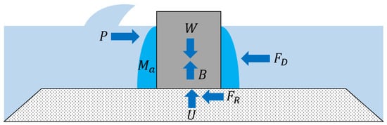
Figure 1.
Force diagram of a caisson under wave.
2.4. Wave Pressure
The dynamic wave load, , of Equation (4) is calculated from the distribution of the static wave pressure by Goda [7]. The wave pressure on the vertical face of a breakwater caisson is expressed in Figure 2.
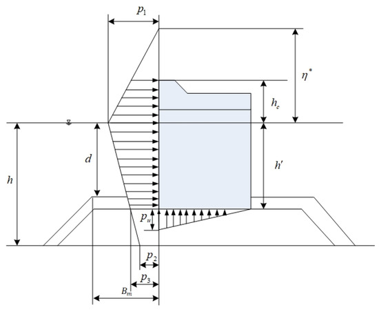
Figure 2.
Wave pressure distribution.
In Figure 2, the pressures are expressed as
where the elevation of from the water level is
in which is the angle of the incident wave, is the correction factor depending on the caisson front face, is the unit weight of seawater, is the design wave height, and is the wavelength. The coefficients of are ~ are as follows:
where is the water depth at a distance of five times the significant wave height () seaward of the breakwater front wall. Then, is replaced by to consider the impulsive force from a head-on breaking wave as:
where is the berm width described in Figure 2.
2.5. Time History of Wave Force
is the horizontal wave load integrated at the caisson face from the bottom to the crest. is the vertical wave load integrated at the caisson bottom from the front to the end. At first, the horizontal wave load is defined by:
where is the pulsating component and is the impulsive component in Goda’s formula. Figure 3 shows the time history of . They are expressed mathematically as:
where is the wave period and is the action time of an impulsive wave defined as:
in which is the wave height in front of the breakwater and is the water depth. In addition, and are the maximum wave pressure obtained from Goda’s formula by applying (correction factor for sinusoidal wave) and . is the reduction factor of a sinusoidal wave due to the increase in the triangular wave pressure. It is defined by:
where ~ is the range of time when the integrand is positive.
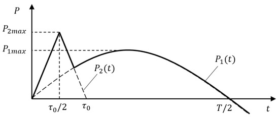
Figure 3.
Time history of the wave force.
The time history of the uplift force, , can be calculated by changing and into and in the procedure from Equations (21) to (27), in which they are the standing and impulsive components of uplift force.
2.6. Tidal Level Time Function during Storm
Figure 4 shows an idealized time history of the tide in the form of a sine function. It is a time function with periodicity between the highest water level (HWL) and the lowest water level (LWL). In Figure 4, TR is the tidal range, i.e., the difference between the HWL and LWL, MWL is the mean water level, and is the period of the tide.
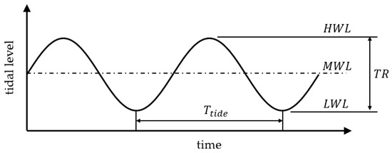
Figure 4.
Time-dependent tidal level.
The conventional approach to the SD calculation of breakwater is performed by analyzing the equation of motion using the wave force during storm conditions with a constant value of tidal level. However, since the tide is a function of time, it also changes during storms. In general, since the typical period of the tide is about 12 h, and assuming that the duration of a storm is two hours, 1/6 of the entire cycle has elapsed, and the tide changes by that much. Therefore, by improving the existing method, it is possible to obtain an accurate SD by considering the temporal change of the tide.
2.7. Expected SD
In Shimosako’s method, it is assumed that 1000 waves attack a breakwater during a storm and that one significant storm occurs every year [11]. Then, the SD of a caisson is thought to accumulate during a lifetime of 50 years. The estimated SD during a lifetime depends on the individual waves generated from the Rayleigh distribution. Because 1000 waves are randomly selected, large and small waves are generated irregularly in some cases. Therefore, the expected value of the SD should be calculated through the so-called Monte Carlo simulation. Figure 5 shows the flowchart of Monte Carlo simulation for the expected SD evaluation. Based on the Weibull distribution, the annual maximum of the significant wave height is generated first. Using the significant wave height, about 1000 consecutive individual waves are generated using the Rayleigh distribution. Time histories of the horizontal wave force and uplift force are developed from the individual wave to obtain the SD of the caisson. If a wave height is larger than a threshold value for sliding, the breakwater slides, and the distance is accumulated during the storm and its lifetime (). This is performed repeatedly in order to average the fluctuation within a random generation. The SD is the averaged value denoted by in Figure 5.
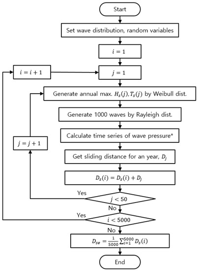
Figure 5.
Flowchart of the Monte Carlo simulation for the expected sliding distance calculation.
3. Time-Varying Tidal Level during Storm
In Equation (4), all properties and loads other than the self-weight, , are affected by the water level, . The tide level is a variable that changes over a period of about 12 h. If the tide-level fluctuation range is small, the tide-level change can be neglected. However, if it is not, an accurate displacement analysis can only be performed by considering the tide-level change effect. In addition, in the case of a storm surge with large tide changes, the tide level must be considered as a variable in order to accurately calculate the breakwater sliding. However, no studies have been published that calculate the SD in a way that takes tide effects into account. In Equation (3), such variables as are dependent on tidal level. In Figure 5, there is no step available that allows researchers to take the tidal level change into account. Actually, the block with the asterisk entitled “Calculate time series of wave pressure” had to be modified to obtain a time-dependent tidal level.
Figure 6 shows that tidal level changes with time. In the figure, the numbers ① through ④ show the four tides at the beginning of a storm. If the storm begins at tide ① or ④, the tidal level falls with time during the storm, while it rises at tide ② and ③. Therefore, the assumption that the tide does not change during a storm can lead to significant errors in understanding breakwater behavior.
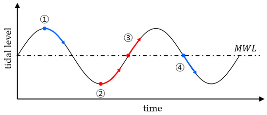
Figure 6.
Tide-level time series.
In Figure 7, continuous wave action was plotted in terms of the time history of the tidal level during a storm. The time at which the wave force acts is the time plus the period of single wave, , at time , and the tidal level changes from to . Therefore, the depth to the caisson bottom, , shown in Figure 2, changes with time, and the wave force must be recalculated by considering the changed tidal level. Also, in Equation (4), all tide-dependent variables must be recalculated. The primary idea of this study is to suggest that the tide-level change should be considered in the sliding calculation process, and a comparison with the existing method is shown through numerical examples in Section 4.
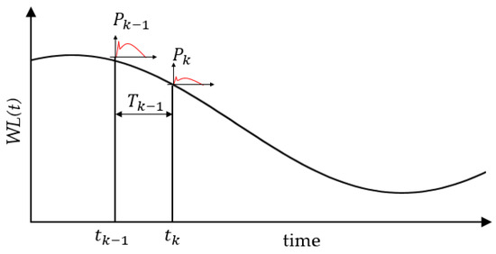
Figure 7.
Consecutive single wave time history plotted on the time history of the tide.
4. Numerical Example
4.1. SD during a Storm Event with a Sinusoidal Tide
Figure 8 shows a vertical-face breakwater designed on a rubble mound with a depth of 17.5 m and a weight of 896.0 tons. The tide level is expressed as a sine function with a period of 12 h from the LWL of 0 m to the HWL of 5 m. The SD is calculated when a significant wave height is 9 m in front of the breakwater. The simulation conditions are summarized in Table 3 and the calculation process is as follows. It is known that continuous waves during a typhoon follow the Rayleigh distribution of Equation (28).
where is the individual wave height and is the scale parameter.
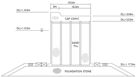
Figure 8.
Side view of caisson-type breakwater.
Table 3.
Summary of simulation conditions.
Assuming that there are 1000 continuous waves during a typhoon, 1000 individual waves following the Rayleigh distribution are generated with a scale parameter of 0.7979, as in Figure 9. The significant wave height of the generated waves is 9 m. The amount of sliding is calculated using the breakwater equation of motion, to which each wave height and randomly determined tide level is applied. At this time, the wave load time series is obtained according to the method in Section 2.5. The final amount of sliding is calculated by accumulating the sliding displacement caused by 1000 waves. This process was repeated 5000 times to obtain the final expected sliding distance due to significant waves with a height of 9 m. At every iteration, a set of 1000 waves was randomly chosen with different seeds in order to simulate random sea waves. Figure 10 shows the convergence curve of 5000 iterations. It shows a large fluctuation at the beginning due to random wave heights, but then the curve converges to average values. The estimated SD during the storm was 1.09 m.
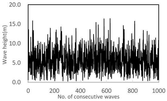
Figure 9.
A total of 1000 waves generated from Rayleigh distribution and of 9 m.
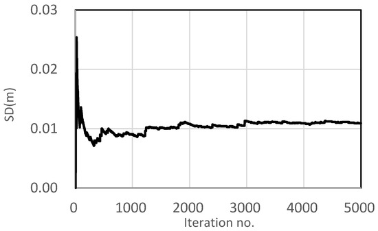
Figure 10.
SD from 5000 iterations due to of 9 m.
To assess how much the SD of a breakwater caused by a storm is affected by the tidal level change, the displacement caused by a single storm was analyzed. At first, it was assumed that a storm begins when the tide is at an LWL, that is, at time ② in Figure 6. The cases are named LWLTI and LWLTD. Next, the storm begins with the tide at an HWL. The beginning time of the storm is ① in Figure 6. The cases are named HWLTI and HWLTD. Finally, the tide begins randomly between the LWL and HWL. These states are named RNDTI and RNDTD. Figure 11 shows the SD due to different significant wave heights with different beginning tidal levels. TI in the case names means that the SD was estimated using a time-independent (TI) tidal level. That is, the tidal levels were fixed during the simulation. TD, on the other hand, indicates a time-dependent (TD) tidal level. That is, the tide was considered to change with time. In an LWLTD situation, the buoyancy increases gradually because the tide rises during storms. Therefore, a larger displacement occurs compared with the LWLTI level. As the wave height increases, the displacement difference becomes larger. When the storm begins at an HWL tide, the opposite occurs. In a HWLTD situation, the tide decreases as the storm progresses and, consequently, buoyancy decreases. Therefore, the SD of an HWLTD level is lower than that of HWLTI. No significant difference was found between the two results obtained with an RNDTI and RNDTD. When the tide is in a descending state at the beginning of a storm, the TD tide increases the SD. However, in an ascending state, it decreases SD. Therefore, if the tide is randomly selected at the storm’s start, the two effects are canceled and the effect of applying a TD tide does not appear. The results are also summarized in Table 4.
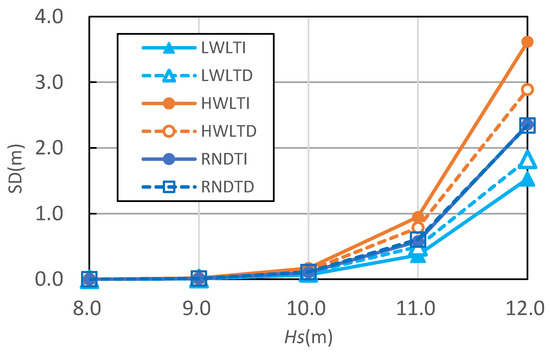
Figure 11.
SD with sinusoidal tide.
Table 4.
SD with a random tidal level at storm start (sinusoidal).
Figure 12 compares the SD ranges when the significant wave height varies from 8.0 m to 12.0 m. Figure 12a shows the SD ranges when the TI tide is used, while Figure 12b gives the SD ranges with the TD tide is used. It can be concluded that the SD ranges were narrowed due to TD tide use. When the significant wave height was 12 m, the SD range decreased by 49% from 2.09 m in (a) to 1.06 m in (b).
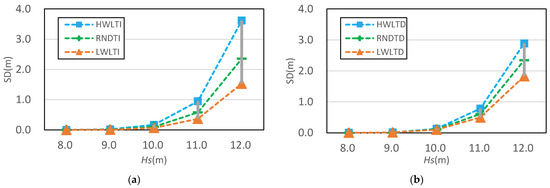
Figure 12.
SD range according to the significant wave height for a TI tide (a) and TD tide (b).
4.2. Sliding Distance during a Storm Event with a Realistic Tide
In this section, a realistic tide function was used to analyze the effect of tide on SD. Figure 13 shows the time history of a realistic tide. It is composed of three periodic components: 12 h, 24 h, and 11.613 h. These were not obtained via measurement but from assumption. The water level due to tide can be expressed as a time function as follows.
where the is 5 m and is 2.5 m. When a more realistic tide function is applied, the SD at the LWL, HWL, and random tide levels are shown in Figure 14. The difference in SD according to the TI and TD tide showed similar a deviation to the case of using a simple harmonic function for tide assessments. Table 5 shows the SD error when the starting tide level is randomly applied. The error was slightly larger than that of the previous section.
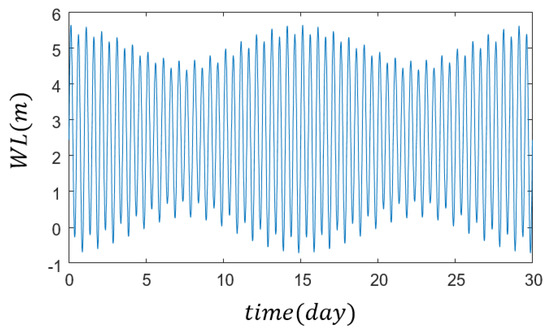
Figure 13.
Water level due to realistic tide.
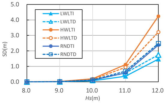
Figure 14.
SD with a realistic tide.
Table 5.
SD with a random tidal level at storm start (realistic).
Figure 15 compares the SD ranges when the realistic tidal level function is used. The results were very similar to those when a simple harmonic function is used for tide. It can be also concluded that the SD ranges have been narrowed due to the tidal level change. When the significant wave height is 12 m, the SD range decreased by 47% from 2.77 m in (a) to 1.47 m in (b).
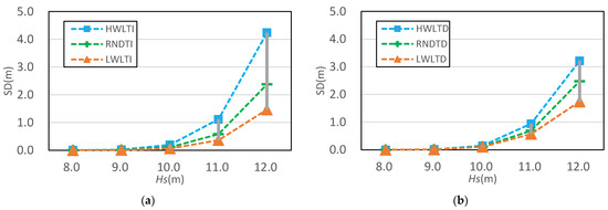
Figure 15.
Range of SD according to tidal dependency on time for TI tide (a), and TD tide (b).
4.3. SD during Breakwater Lifetime
To check the effect of tide on the SD during the lifetime of a breakwater, the SD was accumulated for 50 years, and the results were compared. The SD was calculated under the assumption that, on average, one significant storm occurred per year. The significant wave height of the storm was generated using the three-parameter Weibull distribution as
where and are shape, scale, and location parameters, respectively. They were chosen as 1.467, 1.301, and 5.902 for use in simulation in this study. Since the design wave height is a 50-year return period significant wave height and corresponds to a non-exceeding probability of 49/50, it is calculated from the above cumulative distribution function as follows:
A set of randomly generated annual maximum of significant wave heights using the Weibull distribution of Equation (30) is shown in Figure 16.
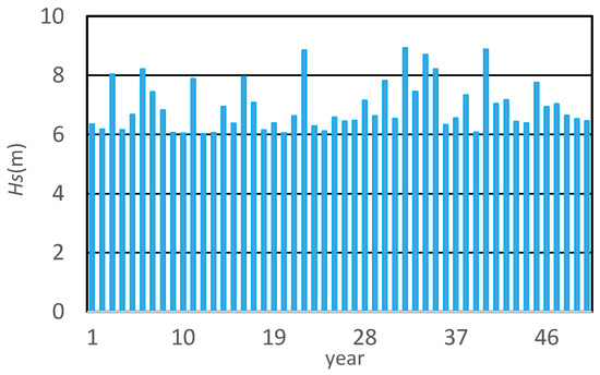
Figure 16.
A realization of annual maximum significant wave heights.
Annually, by using the maximum significant wave, 1000 waves are generated during a typhoon, and the amount of SD is calculated by each wave and accumulated to obtain the annual SD. Assuming an average of one typhoon for 50 years, the total SD during the design life can be calculated. The expected SD is obtained by performing this process more than 5000 times and averaging the results. As shown in Table 6, the expected SD was considered according to the time change of the tide level. Although the TD shows a 2.7% smaller SD than TI, there is little deviation. The reason for this is that the time change effect of the tide does not appear when randomly selecting the tide level during storms for 50 years.
Table 6.
SD with the random beginning of tidal level (sinusoidal).
5. Conclusions
The influence of the tide level on the SD of a breakwater was first shown via numerical analysis. When estimating the SD of a breakwater due to a storm, the SD increased as the tidal level increased. The minimum SD occurred at an LWL, and the maximum SD occurred at an HWL.
Secondly, the primary idea of this study was to propose an innovative approach to considering tidal level change according to the time required for an SD calculation during a storm. In this method, when applying a consecutive wave force to a breakwater, the tidal level is newly updated at the beginning of each wave force. Updating the tide level means that the added mass, buoyancy, wave force, and uplift force into the equation of the motion of the breakwater are newly calculated according to the time function of the tidal level. When a storm begins at an LWL, the tide rises during the storm. Then, buoyancy, wave force, etc., increase accordingly, resulting in larger SDs than those obtained without considering the tidal level change. The opposite phenomenon is found when the storm begins at an HWL. As a result, the difference between the minimum and maximum values of the SD according to tidal level becomes narrower when the change in tidal level is taken into account in the SD calculation process.
From a practical point of view, there is a problem in that the tidal level cannot be predicted in advance at the time of storm occurrence. Hence, the estimation of 50-year SD during the lifetime of the caisson is usually performed by assuming a random tide level. Considering random tide levels during a lifetime shows little difference from the tidal level change. In this case, it is considered more reasonable to prepare for disasters by estimating both the lowest SD from the LWL and the highest SD from the HWL, not by estimating a single SD from a random tide level. In addition, the water level during a storm is affected not only by the tidal level but also by the storm surge. Therefore, a more accurate SD estimation will be possible if the tidal level and the storm surge are taken into account at the same time.
Author Contributions
Conceptualization, D.-H.K.; methodology, D.-H.K.; software, D.-H.K.; validation, J.-W.C.; formal analysis, D.-H.K.; data curation, J.-W.C.; writing—original draft preparation, D.-H.K.; writing—review and editing, D.-H.K.; supervision, D.-H.K. All authors have read and agreed to the published version of the manuscript.
Funding
This research was a part of the project titled ‘Development of Disaster Control and Aging Management Method for Port Infrastructure’ (20210603), funded by the Ministry of Oceans and Fisheries, Republic of Korea.
Conflicts of Interest
The authors declare no conflict of interest.
References
- Gao, J.; Shi, H.; Zang, J.; Liu, Y. Mechanism analysis on the mitigation of harbor resonance by periodic undulating topography. Ocean Eng. 2023, 281, 114923. [Google Scholar] [CrossRef]
- Gao, J.; Ma, X.; Dong, G.; Chen, H.; Liu, Q.; Zang, J. Investigation on the effects of Bragg reflection on harbor oscillations. Coast. Eng. 2021, 170, 103977. [Google Scholar] [CrossRef]
- Yamamoto, T.; Yasuda, T.; Oguma, K.; Matsushita, H. Numerical simulation of scattering process of armour blocks on additional rubble mound behind breakwater during tsunami overflow using SPH method. Comp. Part. Mech. 2022, 9, 953–968. [Google Scholar] [CrossRef]
- Zhai, G.; Liu, J.; Ma, Z.; Teh, H. A numerical study of the damage process of armour bricks on wave overtopping using a coupled SPH-DEM method. Comp. Part. Mech. 2023. [Google Scholar] [CrossRef]
- Goda, Y. A Reliability Design Method of Caisson Breakwaters with Optimal Wave Heights. Coast. Eng. Japan 2000, 42, 357–387. [Google Scholar] [CrossRef]
- Loginov, V.N. Evaluation of the pressure impulse on vertical structures subject to breaking waves. Tr. Soiuzmorniiproekta 1962, 2, 47–59. (In Russian) [Google Scholar]
- Goda, Y. New wave pressure formulae for composite breakwater. In Coastal Engineering; ASCE: New York, NY, USA; Copenhagen, Denmark, 1974; pp. 1702–1720. [Google Scholar]
- Oumeraci, H.; Kortenhaus, A. Analysis of dynamic response of caisson breakwaters special issue on vertical breakwaters. Coast. Eng. 1994, 22, 159–183. [Google Scholar] [CrossRef]
- Lundgren, H. Wave shock forces: An analysis of deformations and forces in the wave and in the foundation. In Research on Wave Action; Delft Hydraulics Lab.: Delft, The Netherlands, 1969; pp. 1–20. [Google Scholar]
- Shimosako, K.; Takahashi, S.; Tanimoto, K. Estimating the sliding distance of composite breakwaters due to wave forces inclusive of impulsive forces. In Coastal Engineering; ASCE: Kobe, Japan, 1994; pp. 1580–1594. [Google Scholar]
- Shimosako, K.; Takahashi, S. Reliability Design Method of Composite Breakwater Using Expected Sliding Distance; Report of the Port and Harbor Research Institute: Yokosuka, Japan, 1998; Volume 37, p. 3. [Google Scholar]
- Cuomo, G.; Lupoi, G.; Shimosako, K.; Takahashi, S. Dynamic response and sliding distance of composite breakwaters under breaking and non-breaking wave attack. Coast. Eng. 2011, 58, 953–969. [Google Scholar] [CrossRef]
- Moriyama, Y.; Washio, T.; Nagao, T. Level I reliability design method based on sliding mount of caisson composite breakwater. Coast. Eng. J. JSCE 2003, 50, 901–905. [Google Scholar]
- Yoshioka, K.; Nagao, T.; Moriyama, Y. A study on the method of setting the partial factor considering the amount of sliding in a caisson type composite breakwater. Coast. Eng. J. JSCE 2005, 52, 811–815. [Google Scholar]
- Kim, D.H. Expected sliding distance of vertical slit caisson breakwater. China Ocean Eng. 2017, 31, 317–321. [Google Scholar] [CrossRef]
- Goda, Y. Dynamic response of up−right breakwater to impulsive force of breaking waves. Coast. Eng. 1994, 22, 135–158. [Google Scholar] [CrossRef]
- Kortenhaus, A.; Oumeraci, H. Simple model for permanent displacement of caisson breakwaters under impact loads. Append. VIII De Groot Et Al Found. Caiss. Break. 1996, 2, 9. [Google Scholar]
- Takahashi, S.; Tanimoto, K.; Shimosako, K. Dynamic response and sliding of breakwater caissons against impulsive breaking wave forces. In Proceedings of the Wave Barriers in Deepwaters Workshop, Yokosuka, Japan, 10–14 January 1994; Port and Harbour Research Institute: Yokosuka, Japan, 1994. [Google Scholar]
- Takahashi, S.; Tsuda, M.; Suzuki, K.; Shimosako, K. Experimental and FEM simulation of the dynamic response of caisson wall against breaking wave impulsive pressures. Coastal Engineering; ASCE: Reston, VA, USA, 1998; pp. 1986–1999. [Google Scholar] [CrossRef]
- Oumeraci, H.; Kortenhaus, A.; Allsop, N.W.H.; De Groot, M.B.; Crouch, R.S.; Vrijling, J.K.; Voortman, H.G. Probabilistic Design Tools for Vertical Breakwaters; Balkema Publishers: Rotterdam, The Netherlands, 2001. [Google Scholar]
- Takahashi, S. Design of Vertical Breakwaters. In Proceedings of the 28th International Conference on Coastal Engineering, Cardiff, UK, 7 July 2002. [Google Scholar]


Disclaimer/Publisher’s Note: The statements, opinions and data contained in all publications are solely those of the individual author(s) and contributor(s) and not of MDPI and/or the editor(s). MDPI and/or the editor(s) disclaim responsibility for any injury to people or property resulting from any ideas, methods, instructions or products referred to in the content. |
© 2023 by the authors. Licensee MDPI, Basel, Switzerland. This article is an open access article distributed under the terms and conditions of the Creative Commons Attribution (CC BY) license (https://creativecommons.org/licenses/by/4.0/).