European Union 2030 Carbon Emission Target: The Case of Turkey

Abstract

Climate awareness caused by the threat of global warming is the number one agenda item for developed and developing economies. Plans developed in this context, environmentally friendly trends in economic activities, and countries’ efforts to adapt to sustainable development have enabled new road maps. The most important of these efforts is the Paris Climate Agreement signed in 2015 and the Green Deal implemented by the European Union (EU) within the framework of this agreement. In this study, the carbon emissions of Turkey, which has important trade relations with the EU, were estimated using machine learning techniques, and a prediction was made for 2030 based on the results obtained. These results were evaluated in line with the targets of the Green Deal. The R² of support vector regression (SVR), which was applied in the model as one of the machine learning techniques, was found to be 98.4%, and it was found to have the highest predictive power. This technique was followed by multiple linear regression (MLR) with a 97.6% success rate and artificial neural networks (ANN) with a 95.8% success rate, respectively. According to the estimates achieved with the most successful model, SVR, Turkey’s carbon emissions are expected to be 723.97 million metric tons (mt) of carbon dioxide (CO₂) in 2030, the target year set by the EU. This level is 42% higher than the target that needs to be achieved given the data existing in 2019. According to these results, Turkey will not be able to reach the targets set by the EU unless it increases its coal-based energy consumption and provides incentives for renewable energy sources.

1. Introduction

The increasing world population given its limited resources, as well as the increase in diversity and per capita consumption, are rapidly changing the natural structure of the planet. It is the atmosphere that is most affected by this change.

The negative effects caused by greenhouse gas emissions are shown to be the most important cause of global climate change. Industrialization and urbanization processes increase greenhouse gas emissions. In addition, fossil fuels, waste, insufficient use of renewable energy, and uncontrolled consumption of natural resources are other factors that trigger the increase in emissions. Carbon dioxide is the most important driving factor of greenhouse gases, which are composed of compounds with heat retention in the atmosphere and cause global warming. The activities carried out by individuals, countries, or organizations ultimately result in carbon emissions into nature [1].

The increasing negative effects of climate change have caused international organizations and countries to take important steps in this regard in recent years. The first awakening in this sense started with the Stockholm conference in 1972. These efforts were later reinforced by the Brundtland Commission Report, the Kyoto Protocol, and the Paris Climate Agreement signed in 2015. The Paris Climate Agreement is historically significant as it is the world’s first comprehensive climate agreement. The agreement, signed by 175 countries responsible for at least 55% of global greenhouse gas emissions, aims to raise socioeconomic awareness about climate change. The increasing environmental awareness associated with the Paris Agreement has caused countries to adopt roadmaps for climate resilience. Having acted for this purpose, the European Union determined a road map under the title ‘Green Deal’ in 2019 to ensure cooperation in mutual trade and economic goals and to fulfill the requirements of the Paris Agreement in sustainable economic transformation. The aim of this document is to reduce greenhouse gas emissions by 50% by 2030 and achieve zero carbon emissions by 2050.

The European Union (EU) reshaped its entire economic policy and determined the actions and sanctions it will impose on other countries with which it has foreign trade relations, along with its member countries. In this context, to prevent carbon emissions and ensure implementation by commercial partners, it designed the Carbon Border Adjustment Mechanism and planned to introduce additional customs duties at the consumption level [2]. With its zero-carbon target, the Green Deal, which serves as a guide for the transition to the circular economy, binds not only the member countries but also the third countries with which the EU has trade relations. With this document, the EU published the sanctions to be applied for noncooperation and clearly stated the rules for the Carbon Border Adjustment Mechanism. The Carbon Border Adjustment Mechanism is an application that establishes foreign connections in parallel with the trading system established for reducing greenhouse gas emissions in manufacturing industry sectors such as iron and steel, aluminum, and fertilizer. For this purpose, the European Union Green Reconciliation Action Plan has been published by Turkey, considering the 2023 development goals. With the plan published in 2021, Turkey determined its own roadmap for green transformation.

The purpose of this study is to predict the carbon emission of Turkey by 2030 with a model already designed in parallel to some of the existing research in the literature for the purpose of evaluating how far Turkey is from reaching the target set in the EU Green Deal as well as to present a model proposal for the countries that have commercial relations with the EU. This makes the study important for decision makers as well as policy practitioners. For this purpose, the predictive power of the model designed in the study was tested by using three machine learning methods: artificial neural networks, support vector regression, and multiple linear regression. The study differs from other studies on carbon emission estimation as it evaluates these models within the framework of the EU’s Green Deal.

In the literature on the subject, forward-looking estimation methods used in the calculations for carbon emissions, greenhouse gas emissions, carbon footprint, and ecological footprint, which are seen as the causes of global warming, were examined. Making accurate predictions and assessments on climate change will be an important step in finding effective solutions to the problem and in implementing the necessary measures.

Baareh (2013) examined the effect of an artificial neural network model on carbon emission estimation. In this study, where four inputs were used (the consumption of global oil, natural gas, and coal as the primary energy sources), the 1982–2000 period was chosen for the training set, and the 2003–2010 period was chosen for the testing set. Manhattan distance, Euclidean distance, and average size of relative error were compared with the predicted and actual values, and the high performance of artificial neural network models was observed. The study emphasized the fact that accurate predictions about climate change could be a useful tool in solving future problems [3].

Radojevic et al. (2013) estimated greenhouse gas emissions for Serbia using the artificial neural network method. In the study conducted to guide decision makers in ensuring sustainable development, data from the 1999–2001 period were used for training, and data from 2002–2007 were used for testing purposes. In the relevant years, greenhouse gas emissions were chosen as an output variable, and gross domestic product (GDP), share of renewable energy sources, gross energy consumption, and energy density were taken as input parameters. The findings were evaluated with R², and a strong correlation was found between the estimate and the actual results. In this research, the strong prediction feature of the artificial neural network method was confirmed. It was emphasized that this could be a guiding method for future-oriented policies [4].

Abdullah and Pauzi (2015) examined the methods used in carbon emission estimation. The aim of their study was to review the literature on methods of estimation used for this purpose. In their study covering the 2003–2013 period, models related to artificial neural networks, gray models, computer simulation, intergovernmental climate change panel (IPCC) modeling, optimal growth models, and fuel analysis were examined, and the most powerful and reliable results were determined. In this study, 40 different factors were examined, and it was determined that the most frequently used variables were energy consumption, GDP, fuel use, population, vehicle use, cement production, agricultural growth, cultivated area size, and workforce variables, and the most preferred methods were found to be artificial intelligence methods. This research was described as a guide for possible future studies [5].

Pabuççu and Bayramoğlu (2016) estimated CO₂ emissions for Turkey with the artificial neural network method. In their study, the estimations for greenhouse gas emissions in EU-28 countries were compared with those in Turkey as a candidate country. For this purpose, the population, GDP, energy production, energy consumption, and energy use were considered as transportation variables of the EU-28 countries and Turkey and were used as inputs in the five-year models for the 1990–2030 period, and carbon equivalent greenhouse gas emissions were estimated for the years 2020, 2025, and 2030. The long time range of the dataset and the extensive coverage of the countries increased the reliability of the study, and the estimates were evaluated with least squares R2 and MSE. According to the highly reliable results, Turkey’s carbon emissions were estimated to be 740.33 million metric tons (mt), 1039.32 mt, and 1244.13 mt for 2020, 2025, and 2030, respectively. In addition, their study emphasized that the findings obtained in the research were well above the value Turkey committed for the year 2030 in the Paris climate agreement [6].

Garip and Oktay (2018) searched for a robust estimation method for calculating future carbon emissions. The dataset of their study, in which random forest and support vector methods were used as the machine learning methods, was applied for the 1965–2014 period. The 1965–2003 period was taken as the basis for training, and the 2004–2014 period was used for testing purposes. In that study, the variables of oil, natural gas, coal, hydroelectricity, renewable energy, and population, which are believed to affect CO₂ emissions, were determined as the inputs of the model. The obtained findings were evaluated with mean absolute error (MAE) and mean absolute percent error (MAPE), and it was observed that the support vector machine method achieved better results [7].

Appiah et al. (2018) carried out carbon emission estimation for four developing countries using artificial neural networks. In their research focused on China, India, Brazil, and South Africa, seven variables were used as inputs: GDP, the crop production index, the animal production index, fossil fuel consumption, renewable energy consumption, and import and export amounts. The dataset of their study was created for the period 1971–2013, and the estimation performance was tested with the mean-square error (MSE), and a high value, 0.0003345, was obtained. As a result, the predictive efficiency of the artificial neural network was proven [8].

Acheampong et al. (2019) estimated carbon emissions for Australia, Brazil, China, India, and America using artificial neural networks. In their study, the quarterly data for the period 1980–2015 were used for the variables of population, economic growth, energy consumption, R&D, financial development, foreign direct investments, foreign trade openness, industrialization, and urbanization, which are considered important factors affecting carbon emissions. In their study, it was determined that the estimations for each country reached a very high R²; hence, the artificial neural network method could be an effective method with low error in the calculation of carbon emissions for these countries. In addition, their study revealed that the developed models and the achieved results can guide international organizations and decision makers in the policies to be followed against climate change [9].

Shabri (2019) searched for a model with the best forecasting performance in short-term carbon emission estimation for Malaysia. In their study where the group method of data handling (GMDH) algorithm, artificial neural network method, and gray model were compared, the models were created to predict one year ahead between 2000 and 2016. The performance of the models was evaluated with least squares, least absolute shrinkage, and selection operator (LASSO) methods. According to the results obtained, the LASSO-GDMH model showed the best performance in the short-term annual carbon emission analysis for Malaysia, and it was stated that the artificial neural network estimation method could be effective in longer-term analyses [10].

Çeşmeli and Pençe (2020) estimated greenhouse gas emissions for Turkey using machine learning methods. In their study, the dataset covering the years 1967–2017 was taken as a time series and tested. In their research, using Poisson Regression, linear regression (LR), artificial neural networks, the adaptive neural fuzzy inference system (ANFIS), and long short-term memory (LSTM) algorithms, greenhouse gas emissions were estimated for the period 2018–2031. A 10-fold cross-validation was applied to the results of the research, and the results were evaluated with RMSE, MAPE, and R² methods. According to their findings, the highest predictive value in the mentioned period was obtained with the LSTM algorithm. It was stated that the estimated emission values were at a high level, and recommendations were provided regarding the necessary measures to be taken [11].

Özhan (2020) estimated the CO₂ emissions in Turkey with time series using artificial neural networks and the exponential smoothing method. In that study, the dataset for the years 1960–2014, which included the greenhouse gas emission (CO₂ equivalent) values of Turkey, was used. This period was divided into two timeframes: 1960–2004 was considered the period for the training set of the data, and 2005–2014 was used as the period for the test set. The Holt linear trend method and the artificial neural network method were applied to both timeframes, and the results were evaluated with RMSE and MAPE. It was observed that the model obtained from artificial neural networks yielded more successful results than the Holt linear trend method, one of the exponential smoothing methods. According to the estimated values until 2021, it was underlined that carbon emissions were fluctuating with a tendency to increase [12].

Quenard and Roumanie (2021) realized ecological footprint estimation using machine learning methods. Different macro variables were used, and a dataset was created for G-20 countries in relation to the 1999–2018 period. In their research, ecological footprint and its share in total and per individual biocapacity were taken as dependent variables, while the population of countries, birth rate, agricultural production, GDP, gross fixed capital formation, renewable energy consumption, total energy consumption, rural population, carbon emissions, and renewable energy consumption were not. Consumption, rural population, particulate matter pollution, degrees of freedom of personal and political rights, and degrees of civil freedom were included in the model as independent variables. At the same time, in the study in which the improved regression and artificial neural network methods were compared, the findings were evaluated with R-square, and root-mean-square deviation (RMSE), and it was observed that the artificial neural network method provided better results. In addition, it was emphasized that machine learning methods could provide realistic results in projections estimating ecological footprints in the future [13].

Jena et al. (2021) carried out their work on carbon emission estimation for 17 countries, which play a key role in the world economy and have the highest emissions, using artificial neural networks. In their study, where data for the 2017–2019 period were used, GDP, the rural population ratio, and foreign trade openness rates were taken as variables affecting carbon emissions. A prediction accuracy of 96% was determined for the obtained results. It was observed that the predictions made with the artificial neural network method were more effective than the predictions made earlier with the linear statistical models. The results showed that the countries with high emissions, such as China, India, Iran, Indonesia, and Saudi Arabia, would reach higher values soon, and the countries with low emission levels, such as Mexico, South Africa, Turkey, and South Korea, would follow an increasing trend, while the emissions in countries such as America, Japan, England, France, Italy, Australia, and Canada would decrease. In addition, their study highlighted that such forecasts could guide countries in the transition process to a green economy [14].

Akyol and Uçar (2021) estimated the carbon footprint of Turkey by using time series data mining methods. Their study aimed to predict greenhouse gas emissions for 2030 and their effects on the economy by comparing the algorithms most often used such as linear regression (LR), multilayer perceptron (MLP), limited minimum optimization, and support vector machine for regression (SMOreg). The values of variables for the 1990–2017 period, which are believed to affect the carbon footprint, namely population, GDP, energy production, and energy consumption, were used as inputs for 2018–2030 estimations. The findings were evaluated with MSE and MAPE statistics; each estimate was compared with the actual values between 2009 and 2017, and it was found that the closest and most reliable estimation algorithm was SMOreg. According to the results, the greenhouse gas emission amount of Turkey in 2030 was determined to be 728,301 metric tons of CO₂. The comparison was performed with the values targeted in the climate protocols, and recommendations were provided with regard to the passage to renewable energy [15].

Shahzad et al. (2021) investigated the impact of weather conditions on cases and deaths during the pandemic period in Istanbul, one of the provinces where COVID-19 spread the most. Between 11 March 2020 and 8 February 2021, the relationships between ozone, sulfur dioxide, nitrogen dioxide, carbon monoxide, air quality pollutants (PM2.5 and PM10), humidity, and temperature values representing environmental quality, and the number of COVID-19 cases were examined. According to the findings obtained through empirical tests, correlation analysis, and quantitative tests using quantitative techniques, it was concluded that changes in air temperatures increase COVID-19 cases and deaths in Istanbul [16].

Qader et al. (2022) carried out their study for Bahrain, where they estimated CO₂ emissions with different methods. In their research using data from the 1933–2018 period, nonlinear autoregressive, Gaussian process regression, the Holt estimation method, and artificial neural networks were applied. The performance of the methods was evaluated with the RMSE, and the artificial neural network model had the lowest level of errors. Their findings showed that the artificial neural network model was the most effective method among others for estimating carbon emissions [17].

Yaglikara (2022) examined the effects of economic, political, and social globalization on the ecological footprint of five member countries of the Association of Southeast Asian Nations. This previous study, where panel cointegration, an augmented mean group (AMG) estimator, and Dumitrescu–Hurlin panel causality tests were used, revealed four independent variables that are believed to be affecting the ecological footprint. According to the findings obtained in this study, in which energy consumption per capita, the economic globalization index, the political globalization index, and the social globalization index were taken as inputs, it was determined that energy consumption increased the ecological footprint, and a one-way causality was found to exist between the ecological footprint and political and social globalization. In addition, a two-way causality was found between energy consumption and political and social globalization and a one-way causality between energy consumption and economic globalization [18].

Udemba et al. (2022) examined Turkey’s capacity to achieve climate goals on the path to economic and sustainable development. In their study covering the years 1985–2018, the symmetric and asymmetric relationship between carbon emissions representing environmental erosion and technological innovation, entrepreneurship, foreign direct investments, hydropower consumption, and economic growth variables representing economic factors were investigated using DOLS and NARDL methods. The long- and short-term effects in the relevant years were analyzed, and the asymmetric effect of hydropower consumption, which has the largest share in renewable energy use, on environmental degradation was also investigated. Their findings show that environmental quality can be improved through renewable energy, technological innovation, foreign direct investment, and entrepreneurial activities while reducing carbon emissions in line with Turkey’s climate targets [19].

Pata and Samour (2022) tested the environmental Kuznets curve (EKC) hypothesis, which reveals the environment–economy relationship, considering the case of France. Their study, which covered the period between 1977 and 2017, investigated the impact of nuclear energy on the load capacity factor for the first time and examined the impact of nuclear and renewable energy on carbon emissions, ecological footprint, and load capacity factor (LCF) with a causality test based on the Fourier approach. According to their findings, it was concluded that the EKC hypothesis is not valid to establish an association between carbon emissions and the increase in load capacity factor, nuclear energy is effective in environmental sustainability, and renewable energy improves environmental quality but has no long-term effect on environmental conditions [20].

Their study is particularly important as it provides a model for non-EU Mediterranean countries with high-volume trade relations with the EU. The European Union’s relations with third countries date back to the 1960s. It established a global Mediterranean Policy in the 1970s and adopted the ‘Revised Mediterranean Policy’ in the 1990s in order to develop its commercial, financial, and political links. This policy covers relations with 12 countries: Turkey, Morocco, Algeria, Tunisia, Malta, Egypt, Jordan, Israel, Lebanon, Syria, Palestine, and Cyprus. Among these countries, the EU has also signed association agreements with Turkey, Malta, and Cyprus [21]. Sandri et al. (2023) stated in their study that the EU Green Deal is expected to lead to increased investments in renewable energy, reduced emissions, green diplomacy, and financing opportunities for green projects and green infrastructure and that it brings attractive opportunities for better cooperation on climate action as well as opportunities for job creation, green growth, and sustainable development [22].

When the literature on the subject was examined, it was found that forward-looking forecasting methods are used in carbon emissions, greenhouse gas emissions, carbon footprint, and ecological footprint calculations, which are indicators for global warming. In previous studies, successful predictions have been achieved, especially with the artificial neural network, gray model, random forest, linear regression (LR), the group method of data handling (GMDH), adaptive neural fuzzy inference system (ANFIS), long short-term memory (LSTM), multilayer perceptron (MLP), and support vector machine (SVM), all of which are considered machine learning techniques. For this reason, in this study, a model consisting of economic, social, and environmental variables is designed, and machine learning techniques ANN, SVR, and MLR are used to predict the carbon emissions of the sample country, Turkey. In this way, the study will provide insights into the extent to which similar countries can comply with the EU’s Green Deal carbon limitations, and which targets should be set for the economic, social, and environmental strategies to be developed for compliance.

The purpose of this study is to predict the carbon emissions of Turkey by 2030 with a model already designed in parallel to some of the existing research in the literature for the purpose of evaluating how far Turkey is from reaching the target set in the EU Green Deal as well as to present a model proposal for the countries that have commercial relations with the EU. This makes the study important for decision makers as well as policy practitioners. For this purpose, the predictive power of the model designed in the study was tested using three machine learning methods: artificial neural networks, support vector regression, and multiple linear regression. This study differs from other studies on carbon emission estimation in that it evaluates these models within the framework of the EU’s Green Deal.

2. Materials and Methods

Machine learning is the modeling of systems with computers that provide predictions by making inferences on data with mathematical and statistical operations. Machine learning is a branch of artificial intelligence used to classify and forecast data by mimicking the way humans learn [23].

In this study, the estimation of the carbon footprint of Turkey in 2030, a developing country, was carried out using machine learning methods. For this purpose, annual data for the 1990–2020 period were used. Artificial neural networks, support vector regression, and multiple linear regression methods were utilized in this study. The decision to use these methods was affected by the characteristics of the models, the suitability of the dataset, and the studies in the literature. The fact that these models produce successful and fast results according to the size and characteristics of the dataset, and the lack of original studies in the literature using these methods, were decisive factors in the selection of these models.

As a developing country, Turkey is a country with an increasing population, leading to an increase in the amount of production and energy use. There are two important reasons for choosing Turkey as the case study in this study. The first one is Turkey’s long-term relations with the EU in terms of trade. Turkey–EU relations started with Turkey’s accession to the European Economic Community in 1959. On 31 December 1995, with the establishment of the Customs Union Agreement, it gained great momentum, and the European Union became the most important trading partner of Turkey. In the years Turkey applied for membership, 40% of its exports and 30% of its imports were to the countries included in the union. According to today’s data, in 2022, the European Union had a 40.6% share in exports, with USD 103.1 billion, and ranked first in imports with a share of 25.6%. In the European Union’s foreign trade, Turkey ranked sixth as the only developing country after developed countries such as the United States, China, Russia, and the United Kingdom [24]. Turkey’s high dependence on this market in the commercial context means that it is highly affected by institutional sanctions in the process of compliance with the Green Deal. For this reason, Turkey was chosen as the sample country with the highest level of trade relations in the analysis. The second reason is Turkey’s geographical location, i.e., its proximity to the EU region. Therefore, with the model designed in this study, researchers and public executives in non-EU countries (UK, Norway, Switzerland, etc.), as well as in North African and Middle Eastern countries, that have extensive trade relations with the EU, will be able to estimate carbon emissions. Thus, they will be able to shape the policies and strategies of their countries according to the carbon limitations set by the EU.

2.1. Dataset

In this study, annual data from 1990, when carbon emission statistics in Turkey began to be recorded, to 2020, the period after the COVID-19 pandemic, which had great economic and social impacts, were used. The data were obtained from an open data-sharing platform of the central data distribution system (Biruni) of the Turkish Statistical Institute (TurkStat). The model was designed by analyzing previous studies in the literature and adding variables that were considered to be related to carbon emissions. The output variable of the model was the estimated tonnage of carbon emissions. The input variables of the model consisted of demographic, economic, energy, agricultural, and animal variables.

The association of the variables used in this study (

Table 1. Variables of the model.

Input Variables	Output Variable
Population	Carbon emissions (tonnes)
Gross domestic product (USD)
Electricity consumption per person (kWh)
Share of renewable energy in total energy (%)
Share of coal in total energy (%)
Share of natural gas in total energy (%)
Share of liquid fuels (gasoline, diesel, etc.) in total energy (%)
Number of internal combustion engine vehicles
Industrial production index (2015 = 100)
Number of cattle
Agricultural area (hectares)
Forest area (hectares)

) with the literature, along with references, is presented in detail below.

The first input variable of the model is the population, which was also used in the studies carried out by Garip and Oktay (2018), Acheampong et al. (2019), Quenard and Roumanie (2021), and Akyol and Uçar (2021) [7,9,13,15].

The second variable is the gross domestic product (GDP), which shows the economic volume of the country. This variable was also used by Radojevic et al. (2013), Pabuççu and Bayramolu (2016), Appiah et al. (2018), Acheampong et al. (2019), Quenard and Roumanie (2021), and Akyol and Uçar (2021) as the input variable [4,6,8,9,13,15]. Another economic variable used as an input in the model is the industrial production index. Although filter chimney systems with carbon capture capability are in operation, fossil-based energy consumption in the industry is common in developing countries such as Turkey. Since the development potential of these countries also focuses on industrial production, this variable was added to the model during the design phase. Acheampong et al. (2019) added a similar variable, the industrialization rate, to their model [9].

Another variable group is related to energy sources and consumption. The ratio of renewable energy to total energy production was included in the model in a similar fashion as in the studies by Radojevic (2013), Garip and Oktay (2018), Appiah et al. (2018), and Quenard and Roumanie (2021) [4,7,8,13]. In addition, the variables related to fossil fuel consumption used by Bareh (2013) and Garip and Oktay (2018) were taken into account in this study as ratios within the total energy shares [3,7]. As for energy consumption, the per capita electricity consumption by year was included in the model, similar to the study by Yaglikara (2022) [18]. In their literature review on carbon emissions, Abdullah and Pauzi (2015) stated that agricultural indicators were frequently used variables and that they increased the predictive power of their model [5]. Based on this previous study, the area of agricultural lands and the number of cattle were added as input variables. As is known, forests are one of the largest carbon absorbers. At the same time, the destruction of forests for the purpose of creating agricultural land reduces carbon absorption. In order to reflect this situation in the model, the surface area of forest land was chosen as an input variable. Finally, the number of vehicles with internal combustion engines used over the years was added to the model. Although the engine and exhaust systems of vehicles with internal combustion engines (especially diesel vehicles) using fossil fuels are produced according to national and international carbon emission standards, the increase in carbon emissions continues in parallel with the increase in the number of vehicles in traffic. Table 1 presents all the variables of the model together.

The statistical summary, including the mean, standard deviation, and ranges of the data utilized for the modeling study, is shown in

Table 2. Descriptive statistics.

	Average	Maximum	Minimum	SD
Population	68,251,387	83,614,362	53,921,758	8,892,094
Gross domestic product (USD)	510,361,786,782	957,783,020,853	130,690,172,297	300,451,945,211
Electricity consumption per person (kWh)	2174	3709	930	892
Share of renewable energy in total energy (%)	31	46	17	8
Share of coal in total energy (%)	31	37	23	4
Share of natural gas in total energy (%)	34	50	15	12
Share of liquid fuels (gasoline, diesel, etc.) in total energy (%)	5	8	0	3
Number of internal combustion engine vehicles	12,399,816	23,448,029	3,750,678	6,273,352
Industrial production index (2015=100)	69	120	33	31
Number of cattle	12,580,168	18,157,971	9,901,458	2,238,392
Agricultural area (hectares)	39,389,935	42,033,000	37,716,000	1,141,581
Forest area (hectares)	21,172,742	23,180,000	20,199,000	877,040

.

2.2. Artificial Neural Networks

Artificial neural networks are mathematical models inspired by the functions of biological neural networks. Owing to the learning feature of ANNs, they can provide solutions to problems that are too complex for traditional techniques [25]. Owing to its learning ability, by using known examples, it can generalize the results to situations that have not been encountered. Artificial neural networks, which are used for purposes such as estimation, classification, and shape completion using numerical information, can be applied in many areas, from financial factors to engineering and medical science, from production applications to fault detection and analysis [26,27].

The artificial neural network algorithm is arranged in multiple layers in order to establish the correlation between inputs and outputs. The first layer is the input layer. The output layer is the last layer. The other layers in between are called the middle layer(s) or hidden layer(s). A network can have more than one hidden layer. The input layer is the terminal through which individual data are delivered to the network. The number of neurons in this layer is equal to the number of data inputs, and each input neuron receives one data point. These data pass to the next layer, the hidden layer, without being processed. Weights are components that show the importance and effect of the information coming to the artificial nerve cell. Each entry has its own weight. The large or small value of weight does not indicate that the input is important or unimportant for the neural network. Weights can have variable or fixed values. The hidden layer is the one that performs the basic functions of the network. Some implementations may have more than one hidden layer in the network. The number of hidden layers and the number of neurons in the hidden layer depend on the problem. This layer receives the data from the input layer, processes them with a function suitable for the problem by multiplying them with weights, and transmits them to the next layer. The addition function calculates the net input received by a cell. Here, the value of each incoming input is multiplied by its own weight and added. Thus, the net input to the network is found [28,29].

$$\mathrm{NET}={\displaystyle \sum }_{\mathrm{i}}^{\mathrm{n}}{\mathrm{x}}_{\mathrm{i}}{\mathrm{w}}_{\mathrm{i}}$$

(1)

Here, x represents the input, w represents the weight value, and n represents the total number of inputs to the neuron.

Another important component of the artificial neuron is the activation function, also known as the threshold function. The activation function outputs the information from the aggregation function. Usually, linear functions, step functions, sigmoid functions, and hyperbolic tangent functions are used as activation functions [30]. The most frequently used activation function is the sigmoid activation function given in Equation (2).

The output layer is the most extreme layer of the network. It processes the data it receives from the hidden layer with the function used by the network and outputs them. The number of neurons in the output layer is equal to the number of outputs of each piece of data that are delivered to the network. The values obtained from this layer are the results obtained from the ANN for the existing problem [31].

$$\mathrm{f}\left(\mathrm{Net}\right)=\frac{1}{1+{\mathrm{e}}^{-\mathrm{NET}}}$$

(2)

As an architectural structure, ANN is divided into two parts: one with feedforward and the other with feedback. In a feedforward architecture, there is a one-way flow of information. Cells are in the form of regular layers from the entrance to the exit. The information coming to the network passes to the input layer and then is processed in the hidden layers and the output layer, respectively, and reaches the output or exit of the network. In a feedback neural network, the output of a cell is not given as an input only to the next layer. But it can be given as an input to any cell in the previous layer or in its own layer [32].

In artificial neural networks, information is contained in the weights of the connections of the neurons in the network. Therefore, it is important how the weights are determined. Since the information is stored throughout the entire network, the weight value of a node does not mean anything by itself. The weights in the entire network should have optimal values. The process to reach these weights is called “training the network”. Accordingly, in order for a network to be trainable, the weight values must be changeable in a dynamic way under a certain rule [33].

2.3. Support Network Regression

Support vector machine (SVM) is a supervised learning method developed by Vapnik and one of the supervised learning methods used for classification and regression [34]. Compared with other traditional learning methods, this method has much better performance and the ability to solve nonlinear problems. The adaptation of SVM for regression, which is widely used for classification problems, was proposed by Smola et al. [35]. The main purpose of support vector regression (SVR) is to draw a line to separate points on a plane. This line is intended to be at the maximum distance for the points of both classes. It is suitable for complex but small- to medium-sized datasets.

SVR is divided into two types: linear and nonlinear regression methods. In the case of linear separability, these bivalent data can be separated directly using an extreme plane. This extreme plane is called the separating hyperplane. The aim of SVR is to ensure that this extreme plane is equidistant from the sample groups in the two separate classes [36]. The linear SVR is shown in Figure 1.

In cases where the data cannot be separated linearly, nonlinear classifiers can be used instead of linear classifiers. In this context, for nonlinear feature spaces, it may be possible to obtain linear classifiers in a new space by transforming the observation vector x_i ϵ Rn into a vector z in a higher-order space [37]. Figure 2 shows the nonlinear SVR.

In the nonlinear SVR, a regression function is expressed as f(x) = wTϕ(x) + b in hyperspace. This function is obtained using the “ϵ-insensitive” loss function. The nonlinear SVR can be obtained by solving the following quadratic programming problem (KPP):

$$\begin{gathered} \underset{\mathrm{w},\mathrm{b},\mathsf{\xi },{\mathsf{\xi }}^{\ast }}{\underbrace{\min }}\frac{1}{2}{||\mathrm{w}||}^2+\mathrm{C}\left({\mathrm{e}}^{\mathrm{T}}\mathsf{\xi }+{\mathrm{e}}^{\mathrm{T}}{\mathsf{\xi }}^{\ast }\right) \\ \left(\mathsf{\varphi }\left(\mathrm{A}\right)\mathrm{w}+\mathrm{eb}\right)-\mathrm{Y}\le \mathrm{e}ϵ+\mathsf{\xi }, \mathsf{\xi }\ge 0\mathrm{e} \\ \mathrm{Y}-\left(\mathsf{\varphi }\left(\mathrm{A}\right)\mathrm{w}+\mathrm{eb}\right)\le \mathrm{e}ϵ+{\mathsf{\xi }}^{\ast },{ \mathsf{\xi }}^{\ast }\ge 0\mathrm{e} \end{gathered}$$

(3)

Here, C is a predetermined parameter and an adjustment parameter that balances the adaptation of errors and the flatness of the regression function. ξ and ξ* are dummy variables that indicate whether the samples enter the ϵ -tube, and ϵ is the unit vector [38].

We obtained the regression function using the Lagrangian multipliers α and α*.

$$\mathrm{f}\left(\mathrm{x}\right)={\displaystyle \sum }_{\mathrm{i}=1}^{\mathrm{n}}\left({\mathsf{\alpha }}^{\ast }-\mathsf{\alpha }\right)\mathrm{K}\left({\mathrm{x}}_{\mathrm{i}},\mathrm{x}\right)+\mathrm{b}$$

(4)

Here, K(x_i, x) = (ϕ(x_i) · ϕ(x)) represents the kernel function and gives the dot product in hyperspace [39]. α and α∗ are Lagrangian multipliers, and they satisfy α_iα_i^∗ = 0, i = 1, 2, …, n. The f(x) function is determined only by samples (support vectors) with Lagrangian multipliers α_i ≠0 or α_i^∗ ≠ 0. It also shows the inputs and outputs of the A = (x₁, x₂, …,x_n) and Y = (y₁, y₂, …, y_n) training set, respectively [40].

2.4. Multiple Linear Regression

Linear regression analysis is used to estimate the value of one variable relative to the value of another variable. The variable that needs to be predicted is called the dependent variable. The variable used to predict the value of the other variable is called the independent variable. There are two types of linear regression analysis: simple regression and multiple regression. While a single explanatory variable is used in simple regression, multiple regression uses many explanatory variables [41].

Multiple linear regression examines the linear relationship between two or more independent variables and one dependent variable. In other words, it is an analysis in which the relationship between a dependent variable and a series of independent variables related to it is revealed [42].

$$\mathrm{y}={\mathsf{\beta }}_0+{\mathsf{\beta }}_{\mathrm{i}+1}{\mathrm{X}}_{\mathrm{i}+1}+{\mathsf{\beta }}_{\mathrm{i}+2}{\mathrm{X}}_{\mathrm{i}+2}+{\mathsf{\beta }}_{\mathrm{i}+3}{\mathrm{X}}_{\mathrm{i}+3}+\cdots .+{\mathsf{\beta }}_{\mathrm{k}}{\mathrm{X}}_{\mathrm{k}}+{\mathsf{\epsilon }}_{\mathrm{i}}$$

(5)

It is defined as i = 1, 2, 3, …, k.

Here, X_ij, j. represents the value of the independent variable at the i level; B_j, j. represents the regression coefficient; e_ij represents the error term; and k represents the number of independent variables. The coefficient β expresses the degree of change that will occur in Y in terms of its own unit in response to a one-unit change in X in its own unit.

3. Results and Discussion

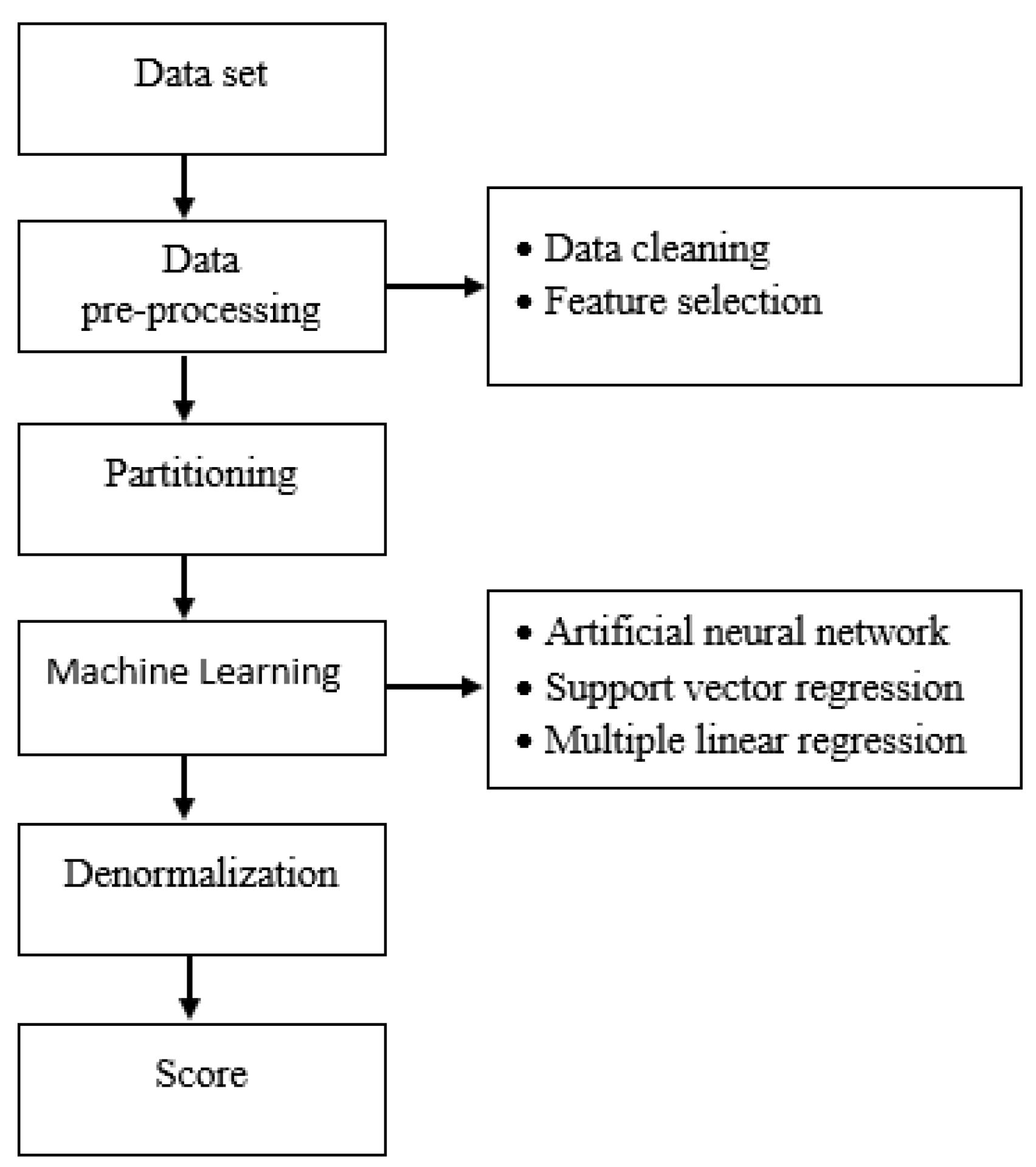
In this study, 30 datasets developed annually between the years 1990 and 2020 were used. A dataset consisting of 12 independent variables was prepared to estimate Turkey’s annual carbon footprint. Three different machine learning methods were used in this study, namely artificial neural networks, support vector regression, and multiple linear regression. The basic workflow of the study is shown in Figure 3.

In machine learning, the efficiency of the training of data can be optimized using preprocessing steps, and thus data are transformed into better forms. By applying the normalization process to raw data, a suitable dataset for training can be prepared. The speed and success rate of the system are directly proportional to the level of preliminary data processing.

The dataset was checked in the preprocessing stage of the dataset, which was the first stage of this study. Inconsistent and erroneous data in the dataset are called noise. To eliminate noise in the data, records containing missing values can be discarded, and a fixed value can be assigned instead of missing values. This fixed value can be found because of a suitable estimation (regression) based on the existing data. In our study, data cleaning was performed to avoid noisy data [43].

The second stage of this study was feature selection. At this stage, the effect of the independent variables used to determine the dependent variable is evaluated, and the independent variables that have much less effect are removed from the dataset [44].

The selection of the attributes is the process of selecting and finding the most useful attributes in the dataset. This process greatly affects the performance of the machine learning model. Feature selection is the selection of subsets of features without sacrificing accuracy. It aims to reduce the level of data by deleting irrelevant and unnecessary data. Its purpose is to improve accuracy by removing unnecessary features. Feature selection is a requirement for any data mining product. A dataset can contain many unnecessary features. Among the existing features, it is necessary to determine the features that affect the result the most, that is, the features that are related to the result. Feature selection works by calculating a score for each attribute and selecting the attributes with the best scores. Most feature selection methods can be divided into three main categories: filter methods, wrapper methods, and embedded methods. The filter method considers the relationship between the feature and the target variable to calculate the importance of the features. As a result of the operations, we filtered our dataset and created a subset by selecting the relevant features [45].

The most used filter methods are the Pearson correlation method and the chi-square method. In the Pearson correlation method, the most widely used correlation measure is the degree of relationship between linearly related variables.

Another phase of the study was the normalization of the data. Normalization is one of the preprocessing techniques used to prepare the dataset for artificial intelligence applications. In this study, the data were normalized between the range of −1 and +1 using the decimal scaling method. In this method, numbers are divided by 10 or by powers of 10 to make them less than 1. As a result, the range is set between −1 and +1 [46].

$${\mathrm{A}}^{\prime }=\frac{\mathrm{A}}{{10}^{\mathrm{j}}}$$

(6)

Here, the real value of A can be defined as the smallest value that makes normalized A^I data, j, and the A value less than one. First, the j values that make the maximum value less than 1 in the columns are found, and new values are obtained by dividing all the elements of the relevant column by the j value.

The data used in the models were divided into two clusters for training and testing purposes. The model was built using the training set based on an assessment of the performance (learning level) of this model using the test set. In this way, predictable labels were obtained for new unlabeled samples with the help of the model [47].

Although there is no definite rule about the separation rate of the data, it is usually decided by trial and error. As a result of the tests performed, the data were divided into two groups based on the rates that provided the highest success rate. Thus, it was decided to use 70% of the data for training and 30% for testing purposes. Taken from the top layer, the linear and random sampling methods are some of the data selection methods that can be used. In this study, the linear sampling method was preferred in data selection to compare the results of the two models.

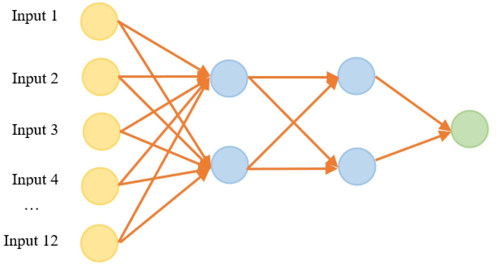
A feedback model was developed using the ANN method. The number of hidden layers and neurons in the model was decided by trial and error. It was observed that the structure with two hidden layers and two neurons in each layer produced more successful results. The structure of the model that was developed is shown in Figure 4.

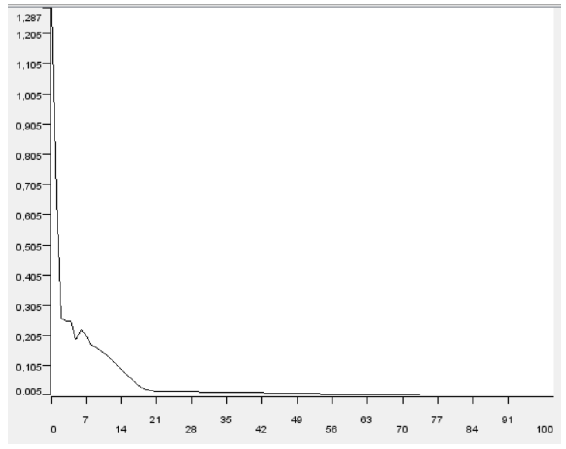
In total, 1000 iterations were performed to obtain the best result in the model. The error curve of the ANN model based on iterations is shown in Figure 5. Figure 5 shows that the error curve decreases nonlinearly. The error curve stabilizes between the 21st and 42nd iterations and reaches the ideal value.

R² (coefficient of determination), RMSE (root-mean-square error), and MAPE (mean absolute percentage error) techniques were used to analyze and interpret the study results.

Nonlinear SVR was used for support vector regression, which is another machine learning method used in this study. A polynomial, hyper-tangent, radial basis function (RBF) was tested for the kernel function, and RBF was preferred in this study since it was determined to be the most successful model. The other parameters of the model were chosen as follows: the overlapping penalty was 100, and the RBF sigma value was 0.1.

To measure the effects of the variables on the system in the multiple linear regression, a significance value was determined first. The variable with the currently highest p-value (the probability value) was determined, and if p > SL, the variable was removed from the system. The model was rebuilt, and then this step was repeated.

When PSL for all variables was reached, elimination was terminated. Since there were no independent values below 0.05 for p-values in the designed model, the model was found to be significant.

R² is a measure of how well the data fit a linear curve. It measures the percentage level, that is, how much the independent variable x explains the dependent variable y in the regression model. R² takes values between 0 and 1 (0R21). If R² equals 1, this indicates that the experimental data provide a perfect linear curve. The higher the R², the better the fit of the regression model [48].

$${\mathrm{R}}^2=1-\frac{\mathrm{Unexplained} \mathrm{Variation}}{\mathrm{Total} \mathrm{Variation}}$$

(7)

RMSE (root-mean-square error) is a quadratic metric that measures the magnitude of error of a machine learning model and is often used to find the distance between the predictor’s predicted values and the true values. RMSE is the standard deviation of the estimation errors (residues). That is, residuals are a measure of how far the regression line is from the data points, and RMSE is a measure of how widespread these residues are. In other words, it indicates how dense the data are around the line that best fits the data. The RMSE formula is shown in Equation (8): Here, n represents the number of data points, and e is the error value [49].

$$\mathrm{RMSE}=\sqrt{\frac{{{\displaystyle \sum }}_{\mathrm{j}=1}^{\mathrm{n}}{\mathrm{e}}_{\mathrm{j}}^2}{\mathrm{n}}}$$

(8)

MAPE (mean absolute percent error) statistics eliminate the disadvantages that may arise when comparing models with different unit values. MAPE is considered superior to other criteria since it expresses the prediction errors as a percentage so that it has a meaning on its own. Models with MAPE < 10% were classified as “very good”, models with 10% MAPE < 20% were classified as “good”, models with 20% < MAPE < 50% were classified as acceptable,” and models with 50% < MAPE were classified as “inaccurate and classified as faulty” [50]. The MAPE formula is shown in Equation (7):

$$\mathrm{MAPE}=\frac{100}{\mathrm{n}}{\displaystyle \sum }_{\mathrm{j}}^{\mathrm{n}}\frac{\left|{\mathrm{e}}_{\mathrm{j}}\right|}{\left|{\mathrm{A}}_{\mathrm{j}}\right|}$$

(9)

The evaluation results of the regression models are presented in

Table 3. Evaluation results of the models.

	ANN	SVR	MLR
R2	0.958	0.984	0.976
RMSE	0.019	0.013	0.016
MAPE	0.063	0.024	0.051

.

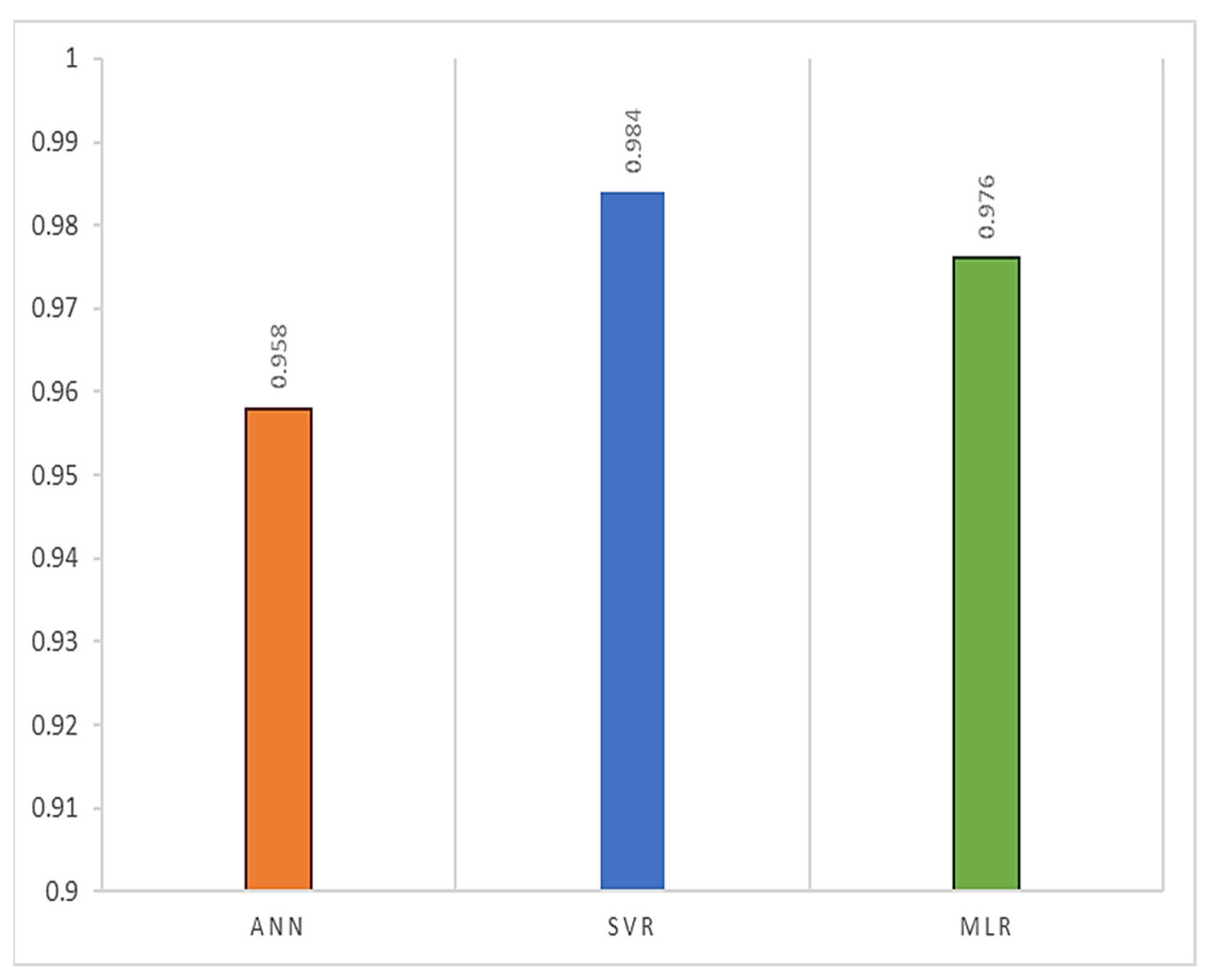
Figure 6 shows the graphical representation of the errors and successes of the models.

Figure 6 shows the coefficient of determination (R²) graphs. An R² of 1, which indicates how well the data fit a linear curve, reveals that the test data provided a linear curve. Based on the results of this study, R² was 95.8% for ANN, 98.4% for SVR, and 97.6% for MLR, and it was found to be very close to the ideal value.

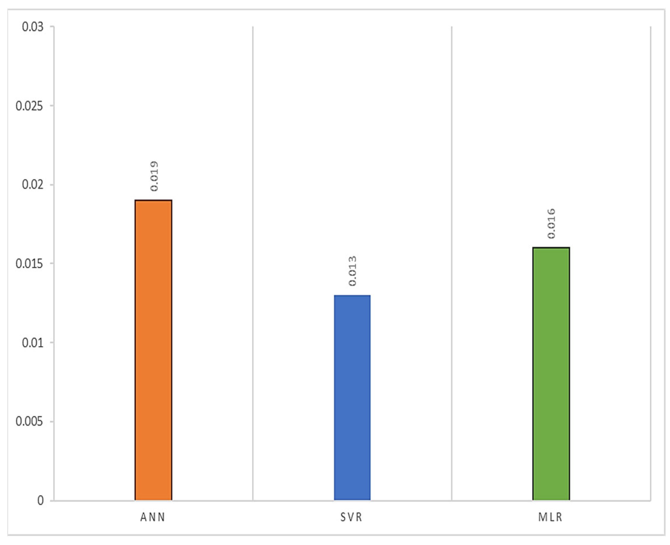
Figure 7 shows the root-mean-square error (MSE) graphs. If RMSE, which is used to find the distance between the estimated values and the actual values, is zero, it means that the model does not make any mistakes. Therefore, it is desired that the RMSE be close to zero. In this study, the RMSE was found to be 0.019 for ANN, 0.013 for SVR, and 0.016 for MLR, which was close to the ideal value.

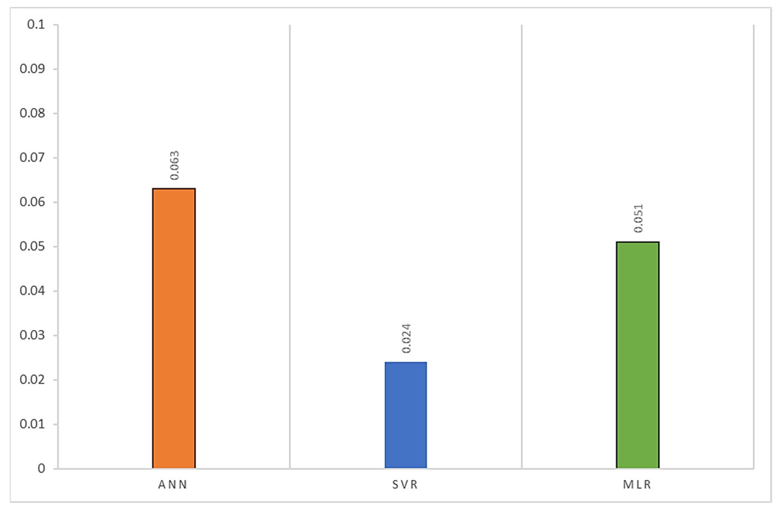
Figure 8 shows the MAPE graphs. Models with a MAPE below 10 percent are considered very good. In this study, this value was 6.3% for ANN, 2.4 for SVR, and 5.1% for MLR, which confirms that the MAPE is very good in all three models.

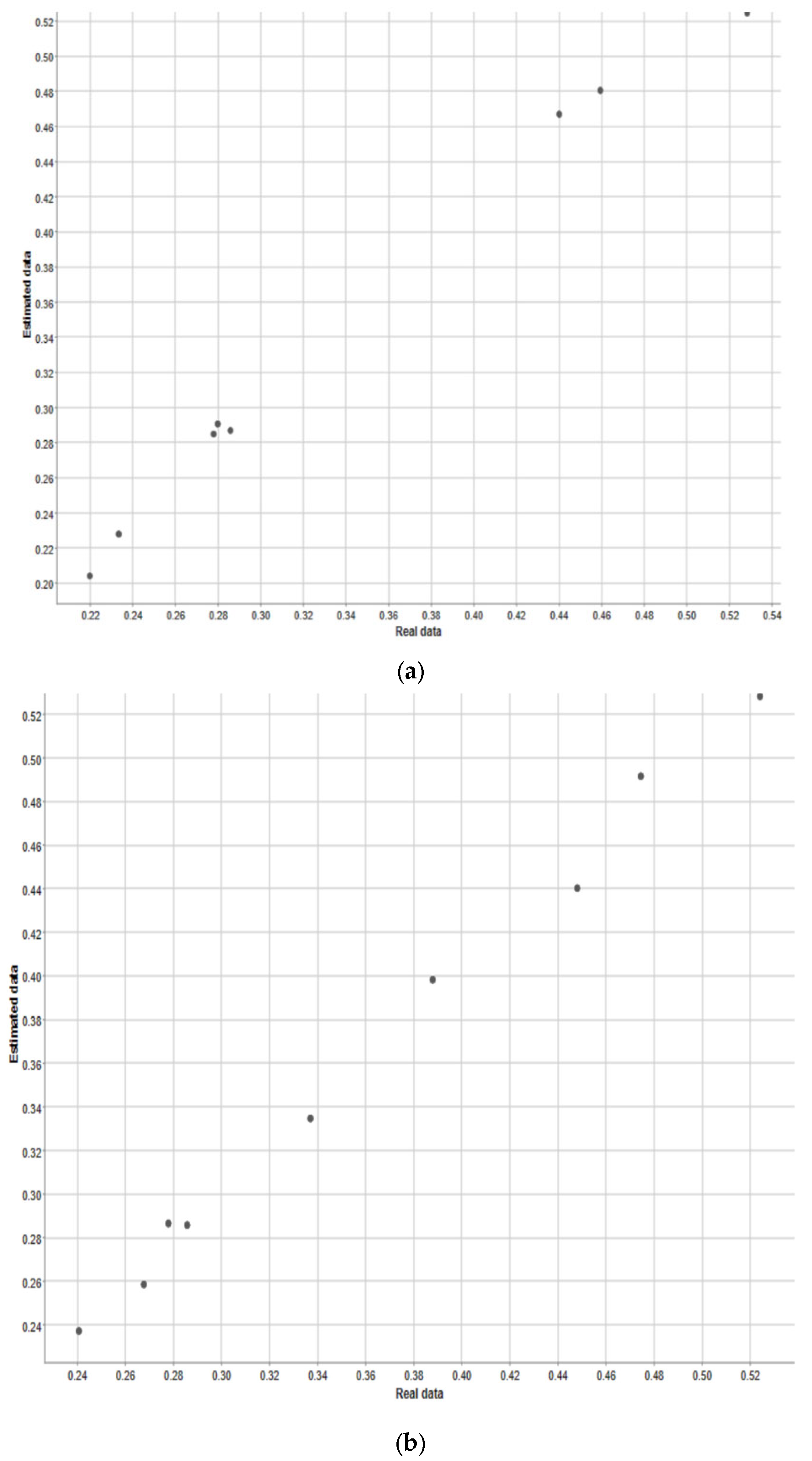
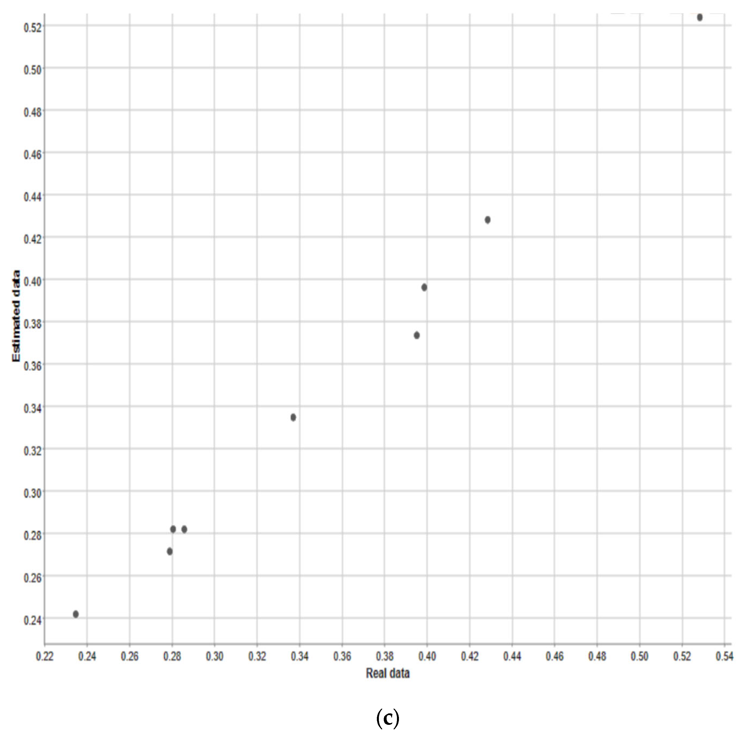
When the error and success values were examined, it was found that the most successful and least erroneous models were SVR, MLR, and ANN, respectively. Figure 9 shows the scatter plots of the models.

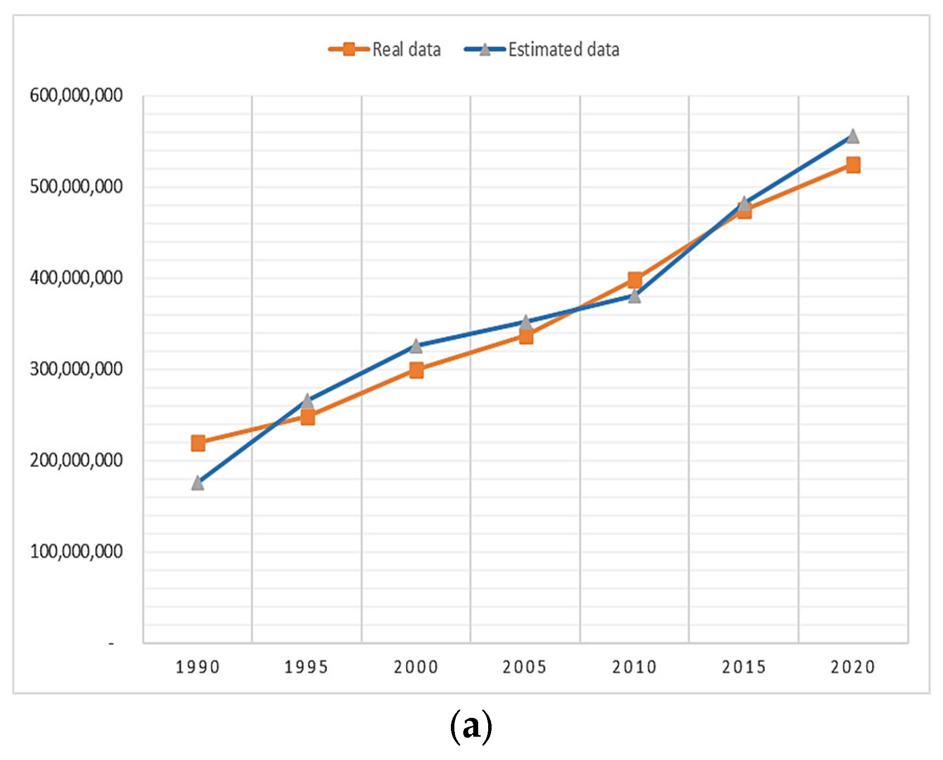
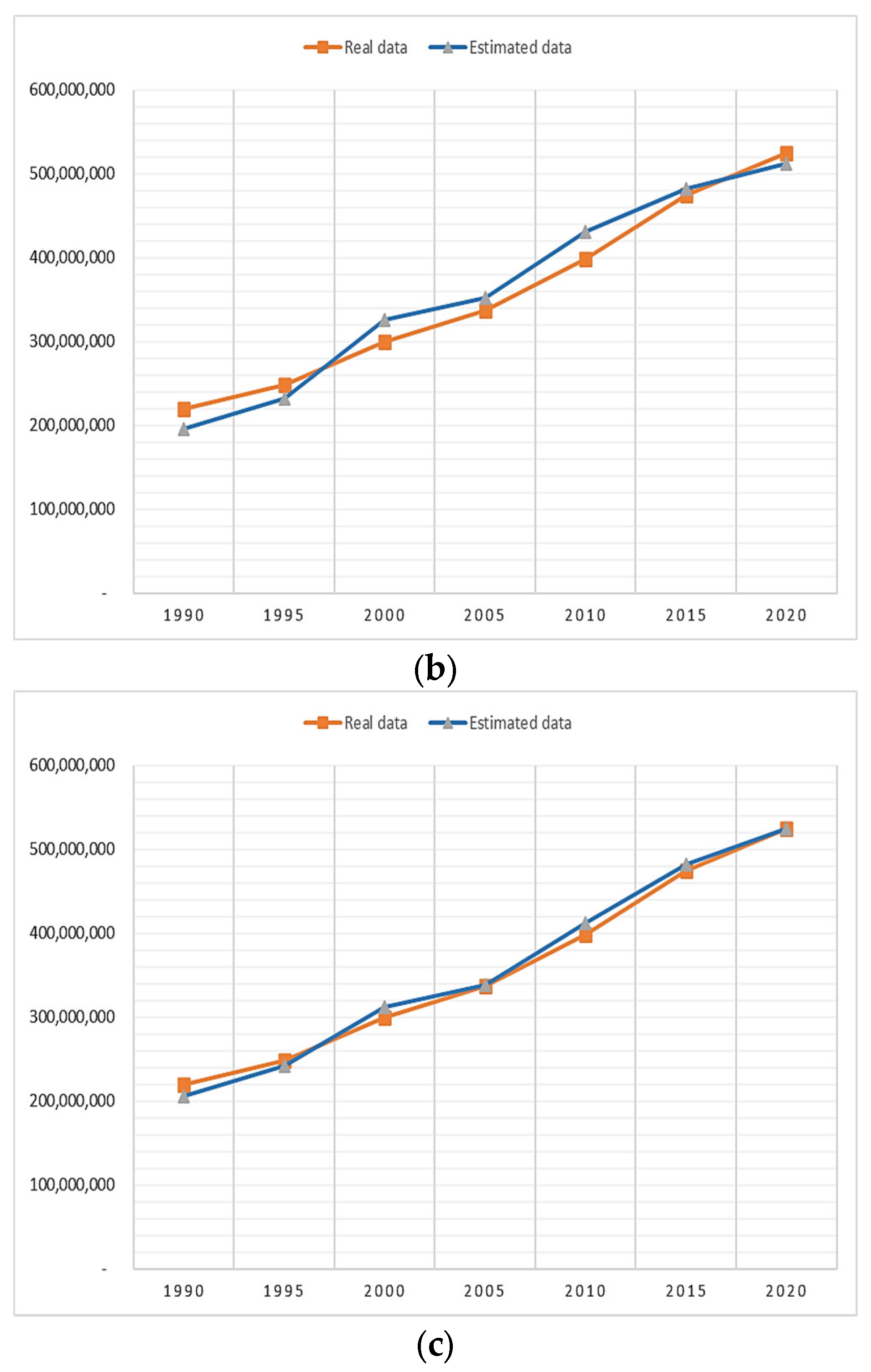
Figure 9 shows the scatter plot of the machine learning models used to estimate Turkey’s annual carbon footprint. In all three models, there was a positive correlation between the methane gas value and the predicted results. Moreover, this link was quite strong. As the value of one of the variables increased, the others increased, and the points clustered near the line. Figure 10 shows the line plots of the models.

Figure 10 shows that the relationship between the actual and predicted values is strong for all three models. When the figures are analyzed in detail, it is seen that the model with the strongest relationship is support vector regression, followed by multiple linear regression and artificial neural networks.

Since the results of the study are normalized, they are expressed between values of 0 and 1. To adapt the results to real values and understand them, denormalization is required.

Table 4. Real and estimated values.

Years	Real Data		Estimated Denormalized Data
		ANN	SVR	MLR
1993	240,635,808	234,546,234	228,985,654	224,423,254
1996	267,662,004	244,524,652	255,885,655	249,365,742
1999	277,879,815	278238,452	275,634,552	280,020,365
2002	285,698,774	290,165,447	276,998,742	299,698,742
2005	336,986,354	351,273,684	337,231,583	358,964,523
2008	387,867,898	389,246,521	392,112,365	391,742,365
2011	428,492,478	444,356,743	437,885,423	424,056,485
2014	459,365,743	465,204,873	474,876,325	440,555,634
2017	528,311,866	521,549,256	539,122,744	524,423,687
2019	508,078,171	516,743,526	500,805,324	504,889,652

shows the actual and estimated values because of denormalization.

As shown in Table 3, the mean error was 2.20% for SVR, 2.33% for ANN, and 2.87% for MLR. It is seen that these values are close to ideal values, and all are acceptable.

4. Conclusions

Carbon emissions, which are one of the most important causes of global climate change, are a significant challenge that needs to be addressed. Especially with the acceleration of coal use after the Industrial Revolution that started in the 18th century, and the increased use of fossil fuel derivatives, together with the increasing use of internal combustion land vehicles in the 19th century, the amount of carbon dioxide in the atmosphere rapidly increased. Since the 1990s, in line with this increase, many national and international organizations have started to develop policies that reduce carbon emissions as a precaution against changes in the climate. At the forefront of these efforts is the Paris Climate Agreement. With this agreement, many countries have been committed to reducing their future carbon emissions. One of the first concrete actions taken within the framework of this agreement is the EU’s Green Deal. This agreement imposes some binding obligations not only on EU countries but also on countries that have commercial activities with EU countries. The countries that have commercial ties with the EU need to reduce their carbon emissions by half by 2030. Otherwise, they will face practices such as high carbon taxation at the border.

The aim of this study was to estimate the carbon emissions of Turkey in 2030, using machine learning techniques, given the fact that Turkey is a country with a high trade volume with the EU (approximately USD 178 Billion as of 2021). In addition, it also aimed at determining how far is Turkey from reaching the target determined by the EU and offering a practical and effective model for other countries that have commercial relations with the EU.

Mediterranean countries emphasize carbon emission reduction and renewable energy policies for the transition to clean energy. For example, Jordan is one of the top three emerging markets globally for clean energy investment. It is important that these investments and transitions are supported and incentivized by the government for clean and reliable energy and its sustainability [51]. While designing the model, the literature was reviewed, and variables used in the existing studies were examined. Considering these studies, the carbon emissions of Turkey were estimated using 12 input variables. Different variables that were considered to affect carbon emissions in the case of Turkey were also included. In this study, ANN, SVR, and MLR machine learning techniques were used to measure the predictive power of the model, as they are assumed to be more effective than other classical statistical techniques. The R2 of SVR was found to be 98.4%, and it was found to have the highest predictive power.

This model was followed by MLR with a 97.6% success rate and ANN with a success rate of 95.8%, respectively. The results of this study are in agreement with the successful predictions made with machine learning techniques in some of the existing studies, such as Radyojevic (2013), Abdullah and Pauzi (2015), Garip and Oktay (2018), Appiah et al. (2019), Roumanie and Quenard (2021), Jena et al. (2021), Akyol and Uçar (2021), and Oader (2022) [4,5,7,8,13,14,15,16].

In this study, three different machine learning techniques were used: SVR, MLR, and ANN. Unlike the previous studies in the literature, it was found that SVR was more successful in terms of the measurement of carbon emissions.

Based on the success of this carbon emission measurement model, it could be a viable model to reach the Green Deal targets for decision makers in developing countries that have commercial relations with the EU, like Turkey.

According to the estimates obtained using the SVR model, the carbon footprint of Turkey is expected to be 723.97 million metric tons (mt) of CO₂ in 2030, the target year determined by the EU. This rate is 42% higher than the target rate that should be achieved according to the data available in 2020. This estimated amount of carbon coincides with other studies of Turkey covering different variables and periods.

Pabuççu and Bayramolu (2016) estimated 740.33 million metric tons (mt) of CO₂ using ANN [6], and Akyol and Uçar (2021) estimated 728.301 million metric tons (mt) of CO₂ using SMOreg [15].

According to the results obtained in this study, when the fossil-based energy sources used in the model were analyzed, it was found that Turkey will not be able to reach the 2030 or 2050 carbon targets if the current use continues, and the use of renewable energy sources is not increased. The development of renewable energy resources, energy efficiency, sustainable agriculture, and changes in the industry and transportation sectors will contribute to the reduction in carbon emissions, which will accelerate Turkey’s transition to a sustainable economy in a short time without compromising its economic growth targets. At the same time, given the huge impact of coal use on carbon emissions, coal consumption for both electricity generation and residential heating needs to be rapidly phased out. Moreover, in line with these objectives, Turkey’s environmental and economic policies need to be redesigned by policymakers in line with sustainable development goals.