Power Source Importance Assessment Based on Load Importance and New Energy Uncertainty

Abstract

With the increasing penetration of new energy sources, the volatility and uncertainty of new energy output can lead to interruptions or fluctuations in the supply of electricity. Power cuts to critical loads can have a significant impact on public safety, social stability, and the economy. Dealing with the effects of uncertainty from new energy sources means we need to find and strengthen the important loads and power sources when designing and operating the power system. Therefore, the assessment of the importance of loads, conventional power sources, and new energy sources is crucial. This paper proposes a power source importance evaluation method based on load importance and new energy uncertainty. The method constructs a load importance evaluation system considering structural characteristics, outage loss, regulation capability, and other factors. To determine the importance of each load, the method uses the ideal solution method and ranks them accordingly. Next, the method calculates the power supply coefficient, which represents the power supply capability of the power source to the critical loads. This calculation involves using the three-point estimation method, which combines the characteristics of the new energy output and the importance of each load. Following that, the evaluation of load importance and the power supply capacity to critical loads is accomplished based on the ideal solution method, taking into account the diversity of power supply characteristics. This comprehensive evaluation allows us to assess the significance of each load and the power supply capability to meet the needs of critical loads, considering the unique characteristics of each power source. Finally, an example analysis is carried out on the IEEE39 to calculate the importance of various types of power sources, which can accurately reflect the power supply capacity of power sources to important loads and verify the validity of the evaluation method. This method provides subsidies for future power system grid planning and operation.

1. Introduction

In order to realize sustainable, green, and healthy development, new energy power generation represented by wind power and photovoltaic has been developed rapidly, and the penetration rate of distributed new energy is also increasing. As the output of new energy is strongly uncertain and volatile due to multiple factors such as weather and geographic location, it poses a big challenge to the reliability of the power supply. At the same time, there are more and more types of power system loads, and each type of load and power source has different sensitivities to power outages. It is difficult to accurately reflect the differences between loads and power sources if they are evaluated only from the topology and electrical characteristics of the nodes themselves. Therefore, in the power system planning process, it is crucial to explore the component importance evaluation method that takes into account the characteristics of both loads and power sources. This ensures a continuous power supply to critical loads.

Currently, most of the studies on the importance of nodes are carried out from the perspective of topological structure characteristics and electrical operation characteristics. The literature [1] proposes a combination of TOPSIS and gray relational analysis methods based on complex networks, which can objectively evaluate the importance of power system loads. Ref. [2] proposes a comprehensive index for identifying the importance of nodes that integrally takes into account the local and global characteristics of the network and evaluates the importance of nodes based on the median method and the point weight method. However, most of the literature mentioned above mainly focuses on the topology perspective when evaluating power system nodes, which often leads to incomplete assessments of load importance. To address this limitation, many researchers have taken node topological characteristics as a starting point and incorporated various electrical indices to achieve a more comprehensive node importance assessment. Ref. [3] weighted SALSA algorithm is an improved node importance evaluation method for power system loads. It is based on node cohesion and considers both the topological structure and the power flow when assessing the importance of nodes in the power system. Ref. [4] calculates the power distribution relationship of the grid based on the power flow tracking method and divides the power distribution to the grid. The importance of subgrids is determined using subgrid structure coefficients, while the importance of nodes is determined through multi-attribute decision making. Subsequently, nodes are extracted and rearranged based on the proportion of importance attributed to subgrids.

In fact, the essence of a node is the export and import of power. The importance of a node has a great relationship with the load and power source connected to it. Therefore, it is necessary to consider the importance of the load and power source on the node to express the importance of the node. Ref. [5] classifies nodes, assessing the importance of load nodes and power nodes separately. It establishes indicators based on the characteristics of components connected to different nodes, thus enhancing the practicality of the method to some extent. The evaluation does not take into account the characteristics of the load itself. Ref. [6] investigates the grid reconfiguration issue. When selecting the power supply for restoring load nodes, they take into account the load level in the load nodes. The importance of the load is then expressed based on the proportion of the load at different load levels, serving as one of the criteria for choosing the load to be restored. However, today’s power system contains more and more types of loads, and it is difficult to make a more detailed comparison of the importance of loads only from the perspective of load levels. Moreover, the role of loads today is no longer just a component that consumes electrical energy. The ability to adjust the power supply has also been gradually discovered, and the ability of the load to participate in the coordination of the source network is increasingly valued [7,8,9].

In view of the above shortcomings of evaluating the load importance only from the topology and electrical characteristics, this paper proposes a power source importance evaluation method based on load importance and new energy uncertainty. The method constructs a load importance evaluation system considering structural characteristics, outage loss, regulation capability, and other factors. To determine the importance of each load, the method uses the ideal solution method and ranks them accordingly. Next, the method calculates the power supply coefficient, which represents the power supply capability of the power source to the critical loads. This calculation involves using the three-point estimation method, which combines the characteristics of the new energy output and the importance of each load. Following that, the evaluation of load importance and the power supply capacity to critical loads is accomplished based on the ideal solution method, taking into account the diversity of power supply characteristics. This comprehensive evaluation allows us to assess the significance of each load and the power supply capability to meet the needs of critical loads, considering the unique characteristics of each power source. Finally, an example analysis is carried out on the IEEE39 to calculate the importance of various types of power sources, which can accurately reflect the power supply capacity of power sources to important loads and verify the validity of the evaluation method. This method provides subsidies for future power system grid planning and operation.

2. Load Importance Indicator Assessment Methodology

2.1. Load Importance Indicators

2.1.1. Load Topology Factor

Since the general load aggregation factor only reflects the degree of aggregation of nodes but not the size of neighboring nodes, Ref. [10] suggests considering the size of neighboring nodes to enhance the aggregation factor metric.

$${\mathrm{C}}_{\mathrm{i}}=\frac{{\mathsf{\lambda }}_{\mathrm{i}}}{\sqrt{{\displaystyle \sum _{\mathrm{j}=1}^{\mathrm{n}}{\mathsf{\lambda }}_{\mathrm{j}}{}^2}}}+\frac{{\mathsf{\theta }}_{\mathrm{i}}}{\sqrt{{\displaystyle \sum _{\mathrm{j}=1}^{\mathrm{n}}{\mathsf{\theta }}_{\mathrm{j}}{}^2}}}$$

(1)

$${\mathsf{\theta }}_{\mathrm{i}}=\frac{\underset{1\le \mathrm{j}\le \mathrm{n}}{\max }\left\{\frac{{\mathrm{c}}_{\mathrm{j}}}{{\mathsf{\lambda }}_{\mathrm{i}}}\right\}-\frac{{\mathrm{c}}_{\mathrm{i}}}{{\mathsf{\lambda }}_{\mathrm{i}}}}{\underset{1\le \mathrm{j}\le \mathrm{n}}{\max }\left\{\frac{{\mathrm{c}}_{\mathrm{j}}}{{\mathsf{\lambda }}_{\mathrm{i}}}\right\}-\underset{1\le \mathrm{j}\le \mathrm{n}}{\min }\left\{\frac{{\mathrm{c}}_{\mathrm{j}}}{{\mathsf{\lambda }}_{\mathrm{i}}}\right\}}$$

(2)

where c_i represents the load aggregation coefficient of node i, θ_i is the normalization function, and λ_i is the sum of node i’s own degree and the degrees of all its neighbors.

The loads approach centrality as follows:

$${\mathrm{J}}_{\mathrm{i}}=\frac{\mathrm{n}-1}{{\displaystyle \sum _{\mathrm{j}\ne \mathrm{i}}^{\mathrm{n}}{\mathrm{d}}_{\mathrm{i}\mathrm{j}}}}$$

(3)

where d_ij is the shortest distance between node i and node j.

Combining Equations (2) and (3) yields the following Equation (4) for the load topology factor:

$${\mathrm{R}}_{\mathrm{i}}=\frac{{\mathrm{C}}_{\mathrm{i}}}{2{\mathrm{C}}_{\max }}+\frac{{\mathrm{J}}_{\mathrm{i}}}{2{\mathrm{J}}_{\max }}$$

(4)

where C_max and J_max are the load aggregation factor and the maximum value of load proximity centrality, respectively.

2.1.2. Load Outage Loss Indicators

Assuming a load node in the network contains N customers, including industries such as industry and commerce, the resulting loss due to a one-hour power cut can be calculated using the following Equation (5):

$${\mathrm{D}}_{\mathrm{lose},\mathrm{i}}=\frac{{\displaystyle \sum _{\mathrm{j}=1}^{\mathrm{N}}{\displaystyle \sum _{\mathrm{t}=1}^{24}{\mathrm{d}}_{\mathrm{lose},\mathrm{j}}{P}_{\mathrm{t},\mathrm{j}}}}}{24}$$

(5)

where D_lose,i denotes the outage loss of the load in the grid, d_lose,j denotes the unit price of the industry outage loss for the j-th customer in the load node, and P_t,j denotes the electricity consumption of the customer j at the t-th hour.

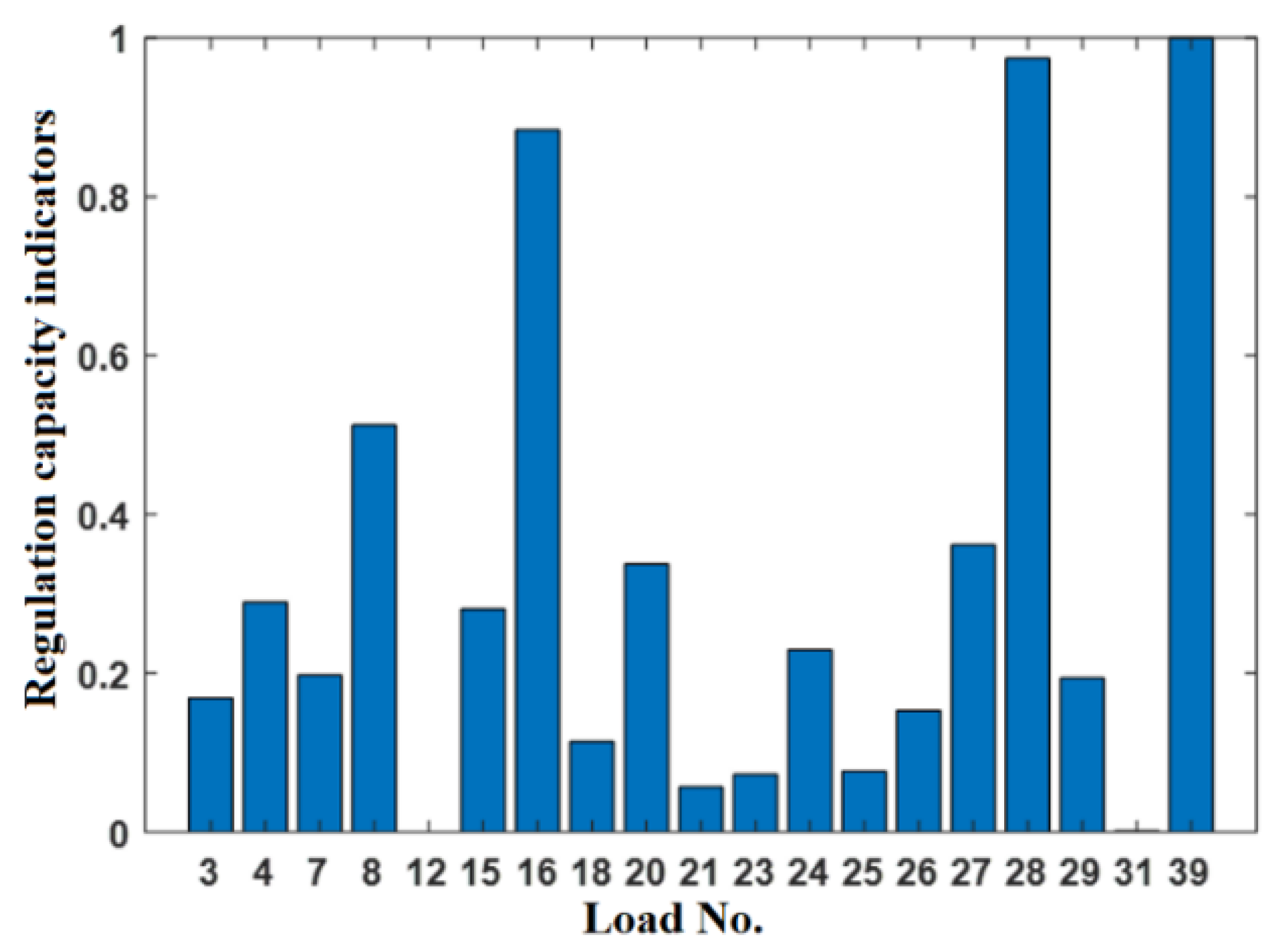
2.1.3. Load Regulation Capacity Indicators

As there are many loads that can be involved in grid regulation in a zone, to simplify the process, this paper only calculates the load regulation capacity for a typical regulated load in a zone. The specific calculation Equation (6) is as follows:

$${\mathrm{A}}_{\mathrm{i}}={\displaystyle \sum _{\mathrm{j}=1}^{{\mathrm{n}}_1}({\mathrm{P}}_{\mathrm{A}\mathrm{L},\mathrm{j}}\cdot {\mathrm{v}}_{\mathrm{A}\mathrm{L}}}{)}^{1/2}+{\displaystyle \sum _{\mathrm{j}=1}^{{\mathrm{n}}_2}{({\mathrm{P}}_{\mathrm{C},\mathrm{j}}\cdot {\mathrm{v}}_{\mathrm{C}})}^{1/2}+{\displaystyle \sum _{\mathrm{j}=1}^{{\mathrm{n}}_3}({\mathrm{P}}_{\mathrm{T}\mathrm{i},\mathrm{j}}\cdot {\mathrm{v}}_{\mathrm{T}\mathrm{i}}}}{)}^{1/2}+{\displaystyle \sum _{\mathrm{j}=1}^{{\mathrm{n}}_4}{({\mathrm{P}}_{\mathrm{E},\mathrm{j}}\cdot {\mathrm{v}}_{\mathrm{E}})}^{1/2}}$$

(6)

where A_i is the index of the adjustable load capacity of the load node i in the grid; P_AL,j, P_C,j, P_Ti,j, and P_E,j represent the adjustable depths of the electrolytic aluminum, silicon carbide, titanium alloy, and electric vehicle users in the load node i, respectively; and v_AL, v_C, v_Ti, and v_E represent the adjustable load rates (adjustable per minute) of the electrolytic aluminum, silicon carbide, titanium alloy, and electric vehicle users in the load nodes, respectively.

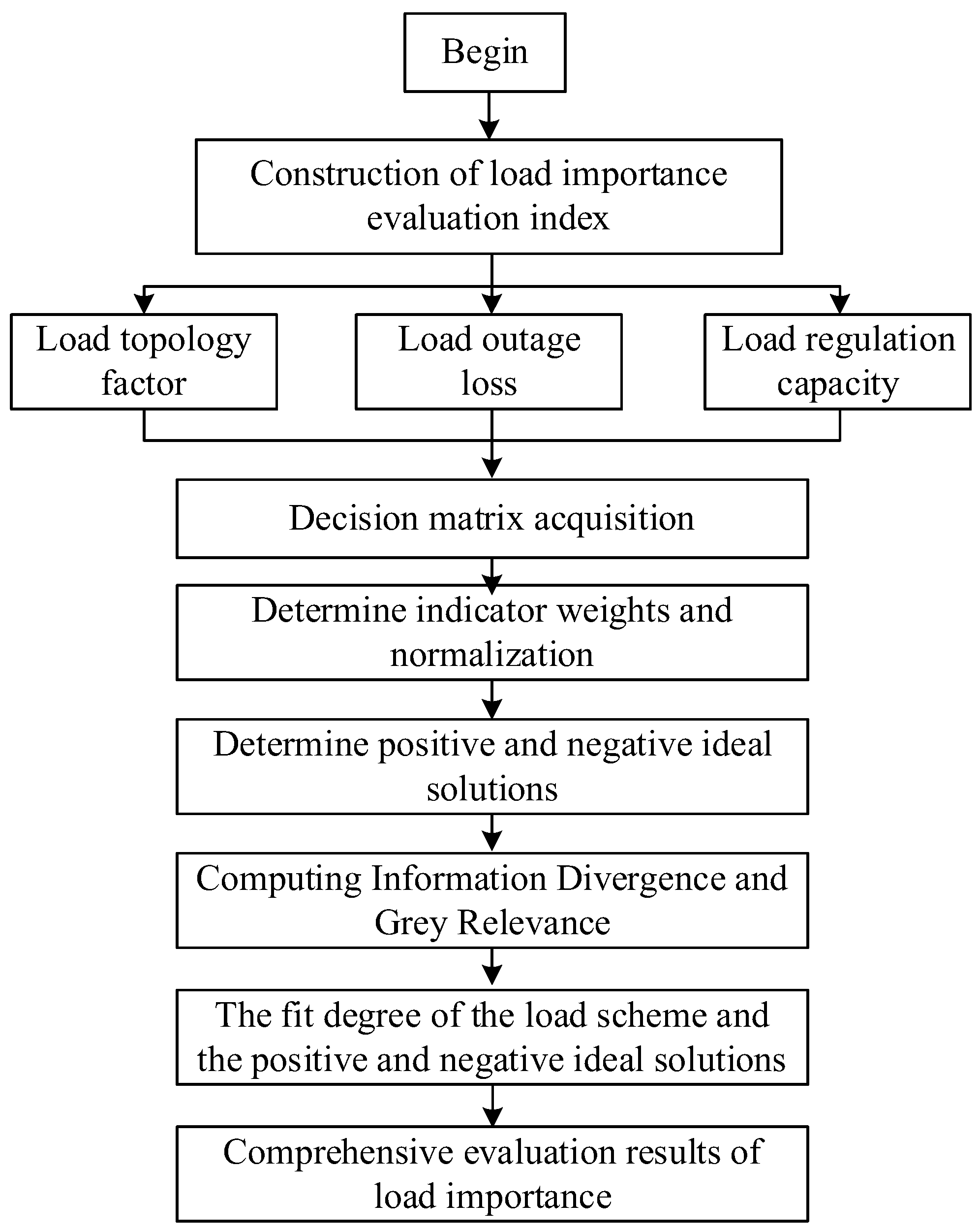
2.2. Load Importance Evaluation Method Based on Ideal Solution Method

The ideal solution method, also known as the TOPSIS algorithm [11], is a method suitable for finding the optimal solution in the case of multiple indicators. In this method, the selection of suitable weights and distance calculation are more important, which may affect the final result of the assessment. In this paper, the ideal solution method is used to calculate the load importance, and the model construction process is as follows:

(1) Calculate the index value of each load by the above index calculation method, and organize to obtain the decision matrix:

$$\mathrm{X}=\left[\begin{array}{cccc}{\mathrm{x}}_{11}& {\mathrm{x}}_{12}& \dots & {\mathrm{x}}_{1\mathrm{m}}\\ {\mathrm{x}}_{21}& {\mathrm{x}}_{22}& \dots & {\mathrm{x}}_{2\mathrm{m}}\\ ⋮& ⋮& & ⋮\\ {\mathrm{x}}_{\mathrm{n}1}& {\mathrm{x}}_{\mathrm{n}2}& \dots & {\mathrm{x}}_{\mathrm{n}\mathrm{m}}\end{array}\right]$$

(7)

where n denotes the number of loads, and m denotes the number of indicators. The column vector in the matrix ${[{\mathrm{x}}_{1,\mathrm{m}},{\mathrm{x}}_{2,\mathrm{m}},\cdots {\mathrm{x}}_{\mathrm{n},\mathrm{m}}]}^{\mathrm{T}}$ denotes the m-th vector of indicator values for each load.

(2) Compromise ratio and ideal TOPSIS-based evaluation of criteria [12] (CRITIC) is a multi-attribute decision-making method for determining the weights, which combines the Gini coefficient and Kendall’s correlation coefficient to indicate the indicator contrast and inter-indicator conflictability. Therefore, the CRITIC method was used to determine the weights of the indicators with the following formula:

The Gini coefficient for the d-th indicator is given in the following equation:

$${\mathrm{G}}_{\mathrm{d}}=\frac{1}{2{\mathrm{n}}^2{\overline{\mathrm{x}}}_{\mathrm{d}}}{\displaystyle \sum _{\mathrm{c}=1}^{\mathrm{n}}{\displaystyle \sum _{\mathrm{k}=1}^{\mathrm{n}}|{\mathrm{x}}_{\mathrm{c}\mathrm{d}}-{\mathrm{x}}_{\mathrm{k}\mathrm{d}}|}}$$

(8)

where ${\overline{\mathrm{x}}}_{\mathrm{d}}$ denotes the average indicator value for the d-th indicator.

The Kendall correlation coefficients between the d-th indicator and the remaining indicators are as follows:

$${\mathrm{T}\mathrm{a}\mathrm{u}}_{\mathrm{d}\mathrm{t}}=\frac{\mathrm{C}-\mathrm{D}}{0.5{\mathrm{n}}^2\frac{\mathrm{M}-1}{\mathrm{M}}}$$

(9)

$$\mathrm{T}\mathrm{a}{\mathrm{u}}_{\mathrm{d}}=\frac{1}{\mathrm{M}}{\displaystyle \sum _{\mathrm{t}=1}^{\mathrm{M}}\mathrm{T}\mathrm{a}{\mathrm{u}}_{\mathrm{d}\mathrm{t}}}$$

(10)

where $\mathrm{T}\mathrm{a}{\mathrm{u}}_{\mathrm{d}\mathrm{t}}$ denotes the Kendall coefficient of the d-th indicator with respect to the t-th indicator; $\mathrm{T}\mathrm{a}{\mathrm{u}}_{\mathrm{d}}$ denotes the total Kendall coefficient of the d-th indicator with respect to the other indicators; M is the lesser of the rows and columns of the matrix; C denotes the number of pairs of consistent elements in the matrix formed by the two indicators, i.e., (${\mathrm{x}}_{\mathrm{c}\mathrm{d}}>{\mathrm{x}}_{\mathrm{k}\mathrm{d}}$, ${\mathrm{x}}_{\mathrm{c}\mathrm{t}}>{\mathrm{x}}_{\mathrm{k}\mathrm{t}}$) or (${\mathrm{x}}_{\mathrm{c}\mathrm{d}}<{\mathrm{x}}_{\mathrm{k}\mathrm{d}}$, ${\mathrm{x}}_{\mathrm{c}\mathrm{t}}<{\mathrm{x}}_{\mathrm{k}\mathrm{t}}$); and D denotes the number of pairs of inconsistent elements in the matrix formed by the two indicators, i.e., (${\mathrm{x}}_{\mathrm{c}\mathrm{d}}>{\mathrm{x}}_{\mathrm{k}\mathrm{d}}$, ${\mathrm{x}}_{\mathrm{c}\mathrm{t}}<{\mathrm{x}}_{\mathrm{k}\mathrm{t}}$) or (${\mathrm{x}}_{\mathrm{c}\mathrm{d}}<{\mathrm{x}}_{\mathrm{k}\mathrm{d}}$, ${\mathrm{x}}_{\mathrm{c}\mathrm{t}}>{\mathrm{x}}_{\mathrm{k}\mathrm{t}}$).

The CRITIC method determines the weights ${\mathsf{\omega }}_{\mathrm{d}}$:

$${\mathsf{\omega }}_{\mathrm{d}}=\frac{\mathrm{T}\mathrm{a}{\mathrm{u}}_{\mathrm{d}}\times {\mathrm{G}}_{\mathrm{d}}}{{\displaystyle \sum _{\mathrm{d}=1}^{\mathrm{m}}(\mathrm{T}\mathrm{a}{\mathrm{u}}_{\mathrm{d}}\times {\mathrm{G}}_{\mathrm{d}})}}$$

(11)

(3) Combine the indicator weights and normalize the decision matrix to obtain the normalized weighted specification matrix Z, calculated as follows:

$${\mathrm{x}}_{\mathrm{i}\mathrm{j}}^{\ast }=\frac{{\mathrm{x}}_{\mathrm{i}\mathrm{j}}-{\mathrm{x}}_{\mathrm{j}\min }}{{\mathrm{x}}_{\mathrm{j}\max }-{\mathrm{x}}_{\mathrm{j}\min }}$$

(12)

$$\mathrm{Z}=\left[\begin{array}{cccc}{\mathsf{\omega }}_1{\mathrm{x}}_{11}^{\ast }& {\mathsf{\omega }}_2{\mathrm{x}}_{12}^{\ast }& \dots & {\mathsf{\omega }}_{\mathrm{m}}{\mathrm{x}}_{1\mathrm{m}}^{\ast }\\ {\mathsf{\omega }}_1{\mathrm{x}}_{21}^{\ast }& {\mathsf{\omega }}_2{\mathrm{x}}_{22}^{\ast }& \dots & {\mathsf{\omega }}_{\mathrm{m}}{\mathrm{x}}_{2\mathrm{m}}^{\ast }\\ ⋮& ⋮& & ⋮\\ {\mathsf{\omega }}_1{\mathrm{x}}_{\mathrm{n}1}^{\ast }& {\mathsf{\omega }}_2{\mathrm{x}}_{\mathrm{n}2}^{\ast }& \dots & {\mathsf{\omega }}_{\mathrm{m}}{\mathrm{x}}_{\mathrm{n}\mathrm{m}}^{\ast }\end{array}\right]$$

(13)

where ${\mathrm{x}}_{\mathrm{i}\mathrm{j}}^{\ast }$ denotes the i-th load normalized to the j-th metric, and ${\mathrm{x}}_{\mathrm{j}\max }$ and ${\mathrm{x}}_{\mathrm{j}\min }$ denote the maximum and minimum values of the j-th metric, respectively.

(4) Determining positive and negative ideal solutions:

$$\begin{array}{l}{\mathrm{Z}}^{+}=[{\mathrm{z}}_1^{+},{\mathrm{z}}_2^{+},\cdots ,{\mathrm{z}}_{\mathrm{m}}^{+}]\\ {\mathrm{Z}}^{-}=[{\mathrm{z}}_1^{-},{\mathrm{z}}_2^{-},\cdots ,{\mathrm{z}}_{\mathrm{m}}^{-}]\end{array}$$

(14)

where ${\mathrm{z}}_{\mathrm{d}}^{+}=\underset{1\le \mathrm{i}\le \mathrm{n}}{\max }{\mathrm{x}}_{\mathrm{c}\mathrm{d}}$, ${\mathrm{z}}_{\mathrm{d}}^{-}=\underset{1\le \mathrm{i}\le \mathrm{n}}{\min }{\mathrm{x}}_{\mathrm{c}\mathrm{d}}$, and ${\mathrm{x}}_{\mathrm{c}\mathrm{d}}$ denotes the elements in row c and column d of $\mathrm{X}$.

(5) Calculate the distance between the [13] loading scheme and the positive and negative ideal solutions using the information dispersion.

$$\left\{\begin{array}{l}{\mathrm{S}}_{\mathrm{i}}^{+}={\displaystyle \sum _{\mathrm{d}=1}^{\mathrm{m}}{\mathsf{\varpi }}_{\mathrm{d}}({\mathrm{z}}_{\mathrm{d}}^{+}\ln \frac{{\mathrm{z}}_{\mathrm{d}}^{+}}{{\mathrm{x}}_{\mathrm{i}\mathrm{d}}}+(1-{\mathrm{z}}_{\mathrm{d}}^{+})\ln \frac{1-{\mathrm{z}}_{\mathrm{d}}^{+}}{1-{\mathrm{x}}_{\mathrm{i}\mathrm{d}}})}\\ {\mathrm{S}}_{\mathrm{i}}^{-}={\displaystyle \sum _{\mathrm{d}=1}^{\mathrm{m}}{\mathsf{\varpi }}_{\mathrm{d}}({\mathrm{z}}_{\mathrm{d}}^{-}\ln \frac{{\mathrm{z}}_{\mathrm{d}}^{-}}{{\mathrm{x}}_{\mathrm{i}\mathrm{d}}}+(1-{\mathrm{z}}_{\mathrm{d}}^{-})\ln \frac{1-{\mathrm{z}}_{\mathrm{d}}^{-}}{1-{\mathrm{x}}_{\mathrm{i}\mathrm{d}}})}\end{array}\right.$$

(15)

where ${\mathrm{S}}_{\mathrm{i}}^{+}$ and ${\mathrm{S}}_{\mathrm{i}}^{-}$ denote the value of the information dispersion distance between load scheme i and the positive and negative ideal solutions, respectively.

(6) Taking into account the various complex direct or indirect coupling relationships in the grid, the gray correlation is introduced to quantify the magnitude of the difference between the load scenarios and the positive and negative ideal solutions.

$$\left\{\begin{array}{l}{\mathrm{h}}_{\mathrm{i}\mathrm{j}}{}^{\pm }=\frac{\underset{\mathrm{m}}{\min }\underset{\mathrm{n}}{\min }\left|{\mathrm{z}}_{\mathrm{d}}^{\pm }-{\mathrm{x}}_{\mathrm{i}\mathrm{d}}\right|+\mathsf{\rho }\underset{\mathrm{m}}{\max }\underset{\mathrm{n}}{\max }\left|{\mathrm{z}}_{\mathrm{d}}^{\pm }-{\mathrm{x}}_{\mathrm{i}\mathrm{d}}\right|}{\left|{\mathrm{z}}_{\mathrm{d}}^{\pm }-{\mathrm{x}}_{\mathrm{i}\mathrm{d}}\right|+\mathsf{\rho }\underset{\mathrm{m}}{\max }\underset{\mathrm{n}}{\max }\left|{\mathrm{z}}_{\mathrm{d}}^{\pm }-{\mathrm{x}}_{\mathrm{i}\mathrm{d}}\right|}\\ {\mathrm{H}}_{\mathrm{i}}{}^{\pm }=\frac{1}{\mathrm{m}}{\displaystyle \sum _{\mathrm{d}=1}^{\mathrm{m}}{\mathsf{\varpi }}_{\mathrm{d}}{\mathrm{h}}_{\mathrm{i}\mathrm{d}}^{\pm }},\mathrm{i}=1,2\dots ,\mathrm{N}\end{array}\right.$$

(16)

where ${\mathrm{h}}_{\mathrm{i}\mathrm{d}}{}^{\pm }$ denotes the gray correlation coefficient between the i-th load scenario and the d-th indicator, ${\mathrm{H}}_{\mathrm{i}}{}^{\pm }$ denotes the gray correlation degree of the i-th load scenario, and $\mathsf{\rho }$ is the resolution coefficient, which is generally 0.5.

(7) Combine the information dispersion value and gray correlation (the weighting this paper selects is 0.5 for each of them) to calculate the fit of each load scenario with the positive and negative ideal solutions so as to obtain the comprehensive fit of each node with the ideal solution.

$$\left\{\begin{array}{l}{\mathrm{Q}}_{\mathrm{i}}^{+}=\mathrm{a}{\mathrm{S}}_{\mathrm{i}}^{-}+\mathrm{b}{\mathrm{H}}_{\mathrm{i}}{}^{+}\\ {\mathrm{Q}}_{\mathrm{i}}^{-}=\mathrm{a}{\mathrm{S}}_{\mathrm{i}}^{+}+\mathrm{b}{\mathrm{H}}_{\mathrm{i}}{}^{¯}\end{array}\right.$$

(17)

$${\mathrm{T}}_{\mathrm{i}}=\frac{{\mathrm{Q}}_{\mathrm{i}}^{+}}{{\mathrm{Q}}_{\mathrm{i}}^{+}+{\mathrm{Q}}_{\mathrm{i}}^{-}}$$

(18)

where $\mathrm{a}+\mathrm{b}=1$, $\mathrm{a},\mathrm{b}\in \left[0,1\right]$; set $\mathrm{a}=\mathrm{b}=0.5$. ${\mathrm{Q}}_{\mathrm{i}}^{+}$ reflects the degree of correlation between the i-th load index and the positive ideal solution; the larger the value, the better the evaluation results. ${\mathrm{Q}}_{\mathrm{i}}^{-}$ is the opposite. ${\mathrm{T}}_{\mathrm{i}}$ denotes the comprehensive closeness, which is used to express the importance of each load; the larger the value, the greater the importance of the load.

The comprehensive assessment process of load importance is shown in Figure 1.

3. Power Source Importance Assessment Based on Load Importance and New Energy Uncertainty

The importance of the power supply is evaluated on the basis of the load importance calculated in Section 2. In the existing literature on power supply importance evaluation, there are evaluations from the perspectives of topological characteristics, rated power, and the generator’s own characteristics, etc. However, many approaches overlook the significance of important loads. The primary purpose of the power supply is to provide electricity to the loads, and the amount of power supplied to important loads serves as the main criterion for assessing the importance of the power supply in the power grid. A power supply integrated power supply coefficient is used to characterize the power supply’s capacity to meet the needs of important loads. Simultaneously, taking into account the distinctions between the features of new energy sources and conventional power sources, if we solely rely on this index to evaluate all types of power sources collectively, new energy sources may encounter inherent drawbacks due to the intermittent nature of their power supply during the assessment. Therefore, in addition to relying on the integrated power supply coefficient as an evaluation index, we also take into account the characteristics of different power sources and select the power source’s own characteristic indexes for different power sources in order to evaluate the importance of different power sources separately.

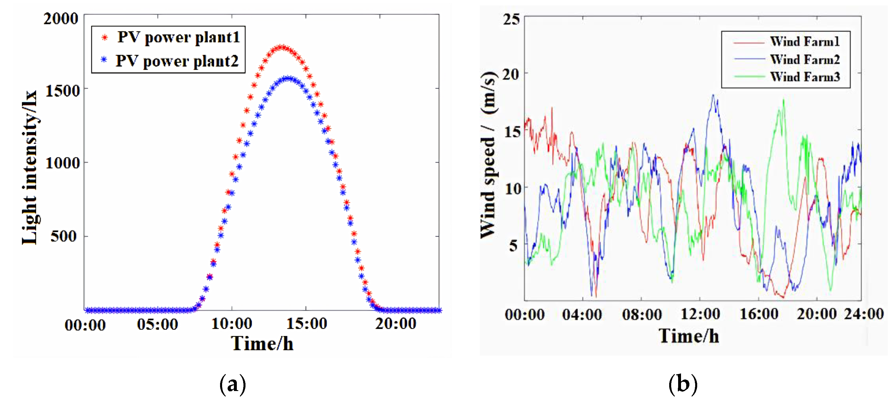
3.1. New Energy System Tidal Current Calculation Based on Point Estimation Method

3.1.1. New Energy Output Uncertainty Model

(1)

Wind Power Output Model

The uncertainty of wind power generation mainly comes from the uncontrollable wind speed in nature. Most of the existing studies use the Weibull distribution [14] to describe the wind speed. The distribution function for the two-parameter Weibull distribution is as follows:

$${\mathrm{F}}_{\mathrm{w}}(\mathrm{v})=1-\exp [-{(\mathrm{v}/\mathrm{c})}^{\mathrm{k}}]$$

(19)

where ${\mathrm{F}}_{\mathrm{w}}(\mathrm{v})$ is the distribution function of the two-parameter Weibull distribution, $\mathrm{c}$ is the scale parameter of the Weibull distribution, $\mathrm{v}$ is the wind speed, and $\mathrm{k}$ is the shape parameter of the Weibull distribution.

(2)

PV power generation output model

The output of the PV genset is highly stochastic, and it converts light energy into electrical energy through PV panels. There is a strong correlation between the variation in light intensity, which has been shown to obey a beta distribution over short time scales or long time scales [15]:

$$\mathrm{f}(\mathrm{r})=\frac{\mathsf{\Gamma }(\mathsf{\alpha }+\mathsf{\beta })}{\mathsf{\Gamma }(\mathsf{\alpha })\mathsf{\Gamma }(\mathsf{\beta })}{(\frac{\mathrm{r}}{{\mathrm{r}}_{\max }})}^{\mathsf{\alpha }-1}{(1-\frac{{\mathrm{r}}_{\mathrm{a}}}{{\mathrm{r}}_{\max }})}^{\mathsf{\beta }-1}$$

(20)

where $\mathsf{\Gamma }(•)$ is the gamma function, $\mathrm{f}(\mathrm{r})$ is the light intensity $\mathrm{r}$ probability density function, α and β are the shape parameters of the beta distribution, and r_max is the local maximum light intensity.

There is a linear relationship between light intensity and PV genset output [16] with the following equation:

$${\mathrm{P}}_{\mathrm{a}}=\left\{\begin{array}{cc}{\mathrm{P}}_{\mathrm{a},\max }\frac{\mathrm{r}}{{\mathrm{r}}_{\max }}\hfill & \mathrm{r}\le {\mathrm{r}}_{\mathrm{e}}\hfill \\ {\mathrm{P}}_{\mathrm{a},\max }\hfill & \mathrm{r}>{\mathrm{r}}_{\mathrm{e}}\hfill \end{array}\right.$$

(21)

where ${\mathrm{P}}_{\mathrm{a},\max }$ indicates the rated power of the PV cell, and ${\mathrm{r}}_{\mathrm{e}}$ is the rated light intensity.

3.1.2. Point Estimation Method

The point estimation method [17], proposed by H.P. Hong in 1998, is one of the probabilistic statistical methods. It allows quick determination of the probabilistic statistical characteristics of output variables when the input variables are independent of each other. The basic idea is to take r; estimation points in each of n independent input random variables, form an evaluation matrix of r × n column vectors, and estimate the probability statistical characteristics of the output variables by calculating the moments of each order of r × n output values. The basic principles of the general point estimation method are described below.

Suppose there is a random variable $\mathrm{X}=({\mathrm{X}}_1,{\mathrm{X}}_2,{\mathrm{X}}_3\dots {\mathrm{X}}_{\mathrm{n}})$, which is the input variable of an n-dimensional random variable function $\mathrm{Z}=\mathrm{f}({\mathrm{x}}_1,{\mathrm{x}}_2,\dots ,{\mathrm{x}}_{\mathrm{n}})$, and in which the random variables are uncorrelated and independent of each other. Let the random variable ${\mathrm{X}}_{\mathrm{i}}$ have mean ${\mathsf{\mu }}_{\mathrm{i}}$ and standard deviation ${\mathsf{\sigma }}_{\mathrm{i}}$; if r values are taken for each variable respectively, the weight of each estimation point is ${\mathrm{p}}_{\mathrm{i},\mathrm{k}}$, and the location coefficient is ${\mathsf{\xi }}_{\mathrm{i},\mathrm{k}}$.

First, each variable is estimated as a point value expression:

$${\mathrm{x}}_{\mathrm{i},\mathrm{k}}={\mathsf{\mu }}_{\mathrm{i}}+{\mathsf{\xi }}_{\mathrm{i},\mathrm{k}}{\mathsf{\sigma }}_{\mathrm{i}}\hspace{1em}\hspace{1em}\mathrm{k}=1,2,\dots \mathrm{r}$$

(22)

The weight of each estimated point is ${\mathrm{p}}_{\mathrm{i},\mathrm{k}}$ and sums to 1 as follows:

$${\displaystyle \sum _{\mathrm{i}=1}^{\mathrm{n}}{\displaystyle \sum _{\mathrm{k}=1}^{\mathrm{r}}{\mathrm{p}}_{\mathrm{i},\mathrm{k}}}}=1$$

(23)

$${\displaystyle \sum _{\mathrm{k}=1}^{\mathrm{r}}{\mathrm{p}}_{\mathrm{i},\mathrm{k}}}=1/\mathrm{n}$$

(24)

The calculation of the estimated point weights ${\mathrm{p}}_{\mathrm{i},\mathrm{k}}$ and positional coefficients ${\mathsf{\xi }}_{\mathrm{i},\mathrm{k}}$ is described below.

Let the j-th order center distance of the input variable ${\mathrm{X}}_{\mathrm{i}}$ be ${\mathrm{M}}_{\mathrm{j}}({\mathrm{x}}_{\mathrm{i}})$, with the following expression:

$${\mathrm{M}}_{\mathrm{j}}({\mathrm{x}}_{\mathrm{i}})={\displaystyle \underset{+\infty }{\overset{-\infty }{\int }}{(\mathrm{x}-\mathsf{\mu })}^{\mathrm{j}}\mathrm{f}(\mathrm{x})\mathrm{d}\mathrm{x}}$$

(25)

Define ${\mathsf{\lambda }}_{\mathrm{i},\mathrm{j}}$ in terms of the ratio of ${\mathrm{M}}_{\mathrm{j}}({\mathrm{x}}_{\mathrm{i}})$ and ${({\mathsf{\sigma }}_{\mathrm{i}})}^{\mathrm{j}}$:

$${\mathsf{\lambda }}_{\mathrm{i},\mathrm{j}}=\frac{{\mathrm{M}}_{\mathrm{j}}({\mathrm{x}}_{\mathrm{i}})}{{({\mathsf{\sigma }}_{\mathrm{i}})}^{\mathrm{j}}}$$

(26)

When $\mathrm{j}=3$, ${\mathsf{\lambda }}_{\mathrm{i},3}$ represents the skewness coefficient of the variable ${\mathrm{X}}_{\mathrm{i}}$. When $\mathrm{j}=4$, ${\mathsf{\lambda }}_{\mathrm{i},4}$ represents the kurtosis coefficient of the variable ${\mathrm{X}}_{\mathrm{i}}$.

The output variables $\mathrm{Z}=\mathrm{f}({\mathrm{x}}_1,{\mathrm{x}}_2,\dots ,{\mathrm{x}}_{\mathrm{n}})$ are subjected to a multivariate Taylor series expansion at each input variable ${\mathrm{X}}_{\mathrm{i}}$. The relationship between each estimated point weight ${\mathrm{p}}_{\mathrm{i},\mathrm{k}}$, the position coefficients ${\mathsf{\xi }}_{\mathrm{i},\mathrm{k}}$, and ${\mathsf{\lambda }}_{\mathrm{i},\mathrm{j}}$ can be obtained by performing a multivariate Taylor series expansion calculation at $\mathrm{k}\times \mathrm{n}$ points:

$${\displaystyle \sum _{\mathrm{i}=1}^{\mathrm{r}}{\mathrm{p}}_{\mathrm{i},\mathrm{k}}}{({\mathsf{\xi }}_{\mathrm{i},\mathrm{k}})}^{\mathrm{j}}={\mathsf{\lambda }}_{\mathrm{i},\mathrm{j}},\hspace{1em}\mathrm{j}=1,2,\dots ,2\mathrm{r}-1,\mathrm{i}=1,2,\dots ,\mathrm{n}$$

(27)

The weights ${\mathrm{p}}_{\mathrm{i},\mathrm{k}}$, location coefficients ${\mathsf{\xi }}_{\mathrm{i},\mathrm{k}}$, and locations of each estimate can be found. When substituting the estimated points into $\mathrm{Z}=\mathrm{f}({\mathrm{x}}_1,{\mathrm{x}}_2,\dots ,{\mathrm{x}}_{\mathrm{n}})$, if you take the estimated values ${\mathrm{x}}_{\mathrm{i},\mathrm{k}}$ for the variables ${\mathrm{X}}_{\mathrm{i}}$, then the other variables take their mean values, and the result of this calculation has a weight of ${\mathrm{p}}_{\mathrm{i},\mathrm{k}}$.

The function $\mathrm{Z}=\mathrm{f}({\mathrm{x}}_1,{\mathrm{x}}_2,\dots ,{\mathrm{x}}_{\mathrm{n}})$ is computed to obtain the $\mathrm{k}\times \mathrm{n}$ output values of the output variable Z. The moment estimates of each order of Z are obtained according to the magnitude of the weights ${\mathrm{p}}_{\mathrm{i},\mathrm{k}}$ at each estimation point:

$$\mathrm{E}({\mathrm{Z}}^{\mathrm{j}})={{\displaystyle \sum _{\mathrm{k}=1}^{\mathrm{r}}{\displaystyle \sum _{\mathrm{i}=1}^{\mathrm{n}}{\mathrm{p}}_{\mathrm{i},\mathrm{j}}\times (\mathrm{f}({\mathsf{\mu }}_1,{\mathsf{\mu }}_2,\dots ,{\mathrm{x}}_{\mathrm{i},\mathrm{k}},\dots ,{\mathsf{\mu }}_{\mathrm{n}},))}}}^{\mathrm{j}}\begin{array}{cc}& \mathrm{j}=1,2,\dots \end{array}$$

(28)

In this paper, the three-point estimation method is used, i.e., k = 3. The calculation process is similar to the above process.

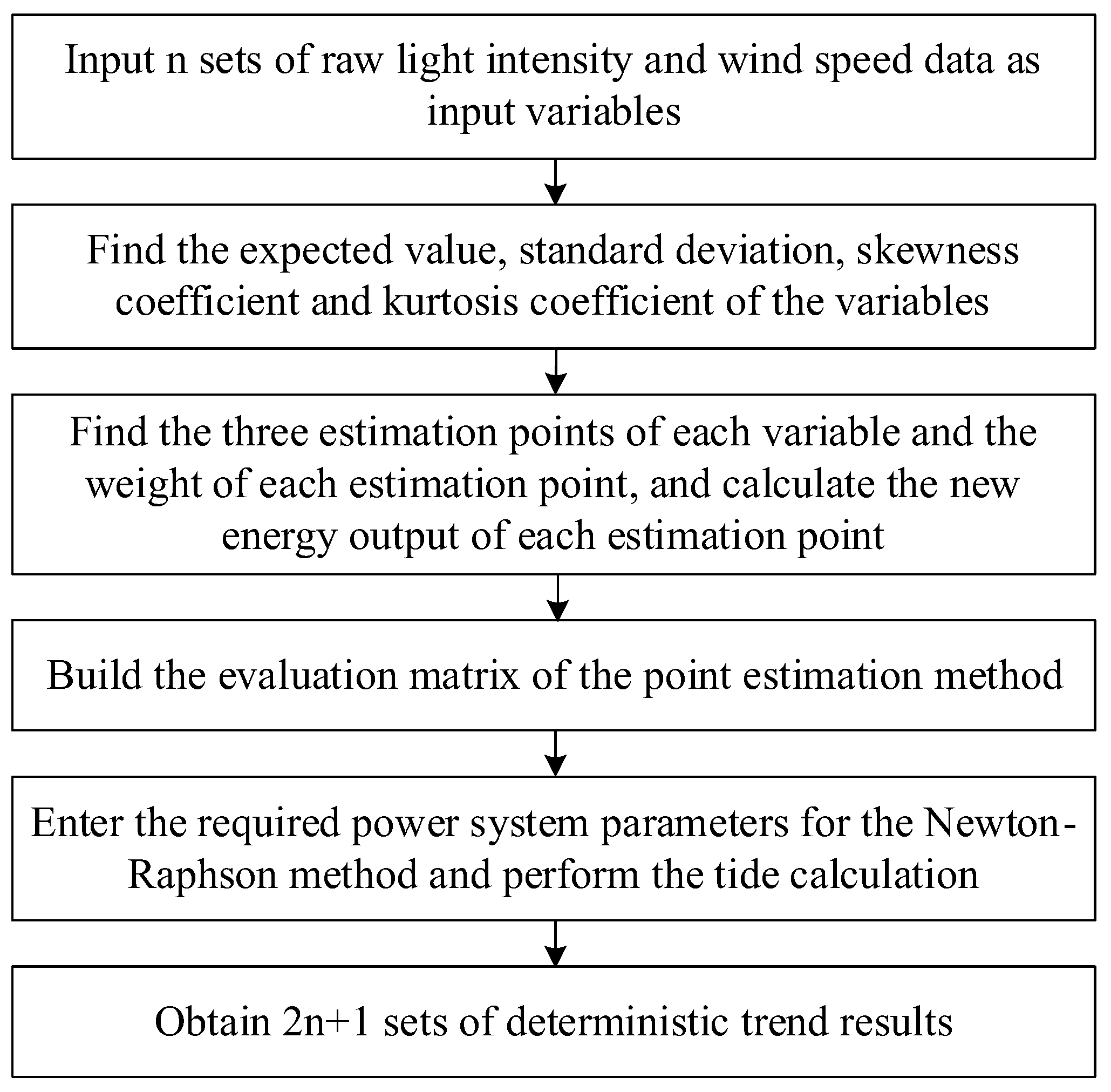
3.1.3. Power Flow Calculation Steps Based on the Point Estimation Method

When the conventional power supply in the power system is replaced by a significant number of new energy sources, such as wind and solar, it introduces uncertainty in the input quantity. Consequently, the conventional power flow calculation method, which relies on fixed input quantities, becomes inappropriate. To address this, the three-point estimation method is considered. It allows us to quickly obtain the probability and statistical characteristics of output variables for functions with multiple random input variables. By combining this method with the Newton–Raphson method, probability power flow calculations can be performed efficiently. The process is shown in Figure 2.

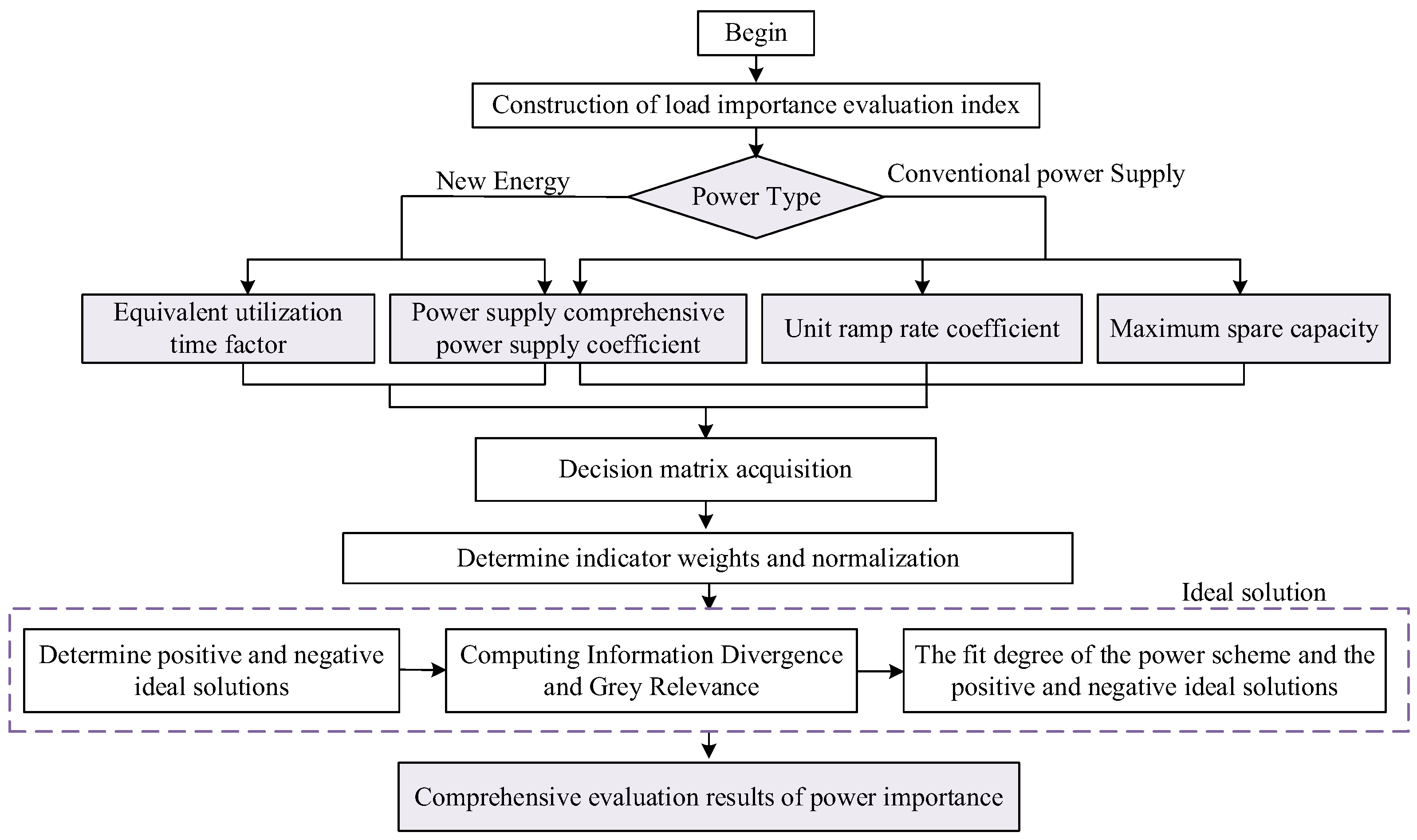
3.2. Power Importance Assessment Based on Load Importance and Power Characteristics

3.2.1. Power Supply Composite Supply Factor Indicator

In the previous part of this paper, the importance of the load was calculated through the three aspects of the load: topology characteristics, power failure loss, and load regulation capability. Based on the above indicators, the product of the power supplied by each generator to different loads and the importance of the load is defined as the comprehensive power supply coefficient of the power supply, and its calculation formula is as follows:

$${\mathrm{G}}_{\mathrm{i}}={\displaystyle \sum _{\mathrm{v}=1}^{2\mathrm{n}+1}{\displaystyle \sum _{\mathrm{j}=1}^{{\mathrm{n}}_{\mathrm{L}}}{\mathsf{\omega }}_{\mathrm{v}}{\mathrm{I}}_{{\mathrm{L}}_{\mathrm{j}}}{\mathrm{P}}_{{\mathrm{G}}_{\mathrm{i}}{\mathrm{L}}_{\mathrm{j}},\mathrm{v}}}}$$

(29)

where ${\mathrm{G}}_{\mathrm{i}}$ denotes the combined power supply coefficient of the power source i; n and ${\mathrm{n}}_{\mathrm{L}}$ denote the number of new energy sources on the grid and the number of loads on the grid, respectively; ${\mathsf{\omega }}_{\mathrm{v}}$ denotes the weight of the v-th tide calculation result; ${\mathrm{I}}_{{\mathrm{L}}_{\mathrm{j}}}$ denotes the importance of the load j; and ${\mathrm{P}}_{{\mathrm{G}}_{\mathrm{i}}{\mathrm{L}}_{\mathrm{j}},\mathrm{v}}$ denotes the power supplied by the power source i to the load j in the v-th tide calculation result.

3.2.2. Power Supply Importance Indicators for Different Power Supply Characteristics

Earlier, the integrated power supply coefficient of power supply was calculated considering the volatility of new energy output and the importance of loads. This coefficient partly represents the significance of the power supply in the power system, where higher importance is given to power supply to important loads. However, due to the distinct characteristics of new energy and conventional power sources, additional indicators are selected for different power sources, considering their specific features. This enables separate evaluations for different power sources, considering their individual attributes:

(1)

Wind farm self-characteristic index

The wind farm’s own characteristic index is the wind farm equivalent utilization time coefficient, whose equation is

$${\mathrm{T}}_{\mathrm{w},\mathrm{i}}=\frac{{\displaystyle {\int }_0^{\mathrm{T}}{\mathrm{P}}_{\mathrm{W},\mathrm{i}}(\mathrm{t})\mathrm{d}\mathrm{t}}}{{\mathrm{P}}_{\mathrm{W},\mathrm{i}}^{\mathrm{N}}\mathrm{T}},\mathrm{i}\in {\mathrm{G}}_{\mathrm{W}}$$

(30)

where ${\mathrm{P}}_{\mathrm{W},\mathrm{i}}(\mathrm{t})$ denotes the output of the i-th wind farm at time t, ${\mathrm{P}}_{\mathrm{W},\mathrm{i}}^{\mathrm{N}}$ denotes the rated installed capacity of the i-th wind farm, ${\mathrm{G}}_{\mathrm{W}}$ denotes the wind farm power pool, ${\mathrm{T}}_{\mathrm{w},\mathrm{i}}$ denotes the wind farm equivalent utilization time factor, and T is the number of wind farm equivalent hours.

(2)

The photovoltaic power station self-characteristic index

Similar to the equivalent utilization time coefficient of wind farms, the index reflecting the equivalent utilization time coefficient of photovoltaic power plants can be expressed as follows:

$${\mathrm{T}}_{\mathrm{S},\mathrm{i}}=\frac{{\displaystyle {\int }_0^{\mathrm{T}}{\mathrm{P}}_{\mathrm{S},\mathrm{i}}(\mathrm{t})\mathrm{d}\mathrm{t}}}{{\mathrm{P}}_{\mathrm{S},\mathrm{i}}^{\mathrm{N}}\mathrm{T}},\mathrm{i}\in {\mathrm{G}}_{\mathrm{S}}$$

(31)

where ${\mathrm{P}}_{\mathrm{S},\mathrm{i}}(\mathrm{t})$ represents the output of the i-th photovoltaic power station at time t, ${\mathrm{P}}_{\mathrm{S},\mathrm{i}}^{\mathrm{N}}$ represents the rated installed capacity of the i-th photovoltaic power station, ${\mathrm{G}}_{\mathrm{S}}$ represents the power source collection of the photovoltaic power station, ${\mathrm{T}}_{\mathrm{S},\mathrm{i}}$ represents the equivalent utilization time coefficient of the photovoltaic power station, and T represents the equivalent hours of the photovoltaic power station.

(3)

The conventional power supply self-characteristic index

➀ Maximum spare capacity, which can be expressed as follows:

$${\mathrm{B}}_{\mathrm{C},\mathrm{i}}={\mathrm{P}}_{\mathrm{C},\mathrm{i}}^{\mathrm{N}}-{\mathrm{P}}_{\mathrm{C},\mathrm{i}}^{\min },\mathrm{i}\in {\mathrm{G}}_{\mathrm{C}}$$

(32)

where ${\mathrm{G}}_{\mathrm{C}}$ represents the set of conventional power supplies, ${\mathrm{P}}_{\mathrm{C},\mathrm{i}}^{\mathrm{N}}$ represents the rated capacity of the i-th conventional power supply, and ${\mathrm{P}}_{\mathrm{C},\mathrm{i}}^{\min }$ represents the minimum technical output of the i-th conventional power supply.

➁ The ramp rate coefficient of the unit can be reflected by the standby unit ramp rate coefficient:

$${\mathrm{M}}_{\mathrm{C},\mathrm{i}}=\frac{{\mathrm{R}}_{\mathrm{i}}}{{\mathrm{P}}_{\mathrm{C},\mathrm{i}}^{\mathrm{N}}},\mathrm{i}\in {\mathrm{G}}_{\mathrm{C}}$$

(33)

where ${\mathrm{R}}_{\mathrm{i}}$ represents the ramp rate of the i-th conventional power supply, ${\mathrm{P}}_{\mathrm{C},\mathrm{i}}^{\mathrm{N}}$ represents the rated capacity of the i-th conventional power supply, ${\mathrm{G}}_{\mathrm{C}}$ represents the set of conventional power supplies, and ${\mathrm{M}}_{\mathrm{C},\mathrm{i}}$ represents the unit ramp rate coefficient of the i-th conventional power supply.

3.3. Evaluation Method of Source-Load Importance Index Based on Ideal Algorithm

In this paper, the ideal solution method is used to calculate the importance of load and power supply. The comprehensive evaluation process of the importance of source and load is shown in Figure 3. The specific process algorithm is consistent with the load-importance solution process.

4. Example Analysis

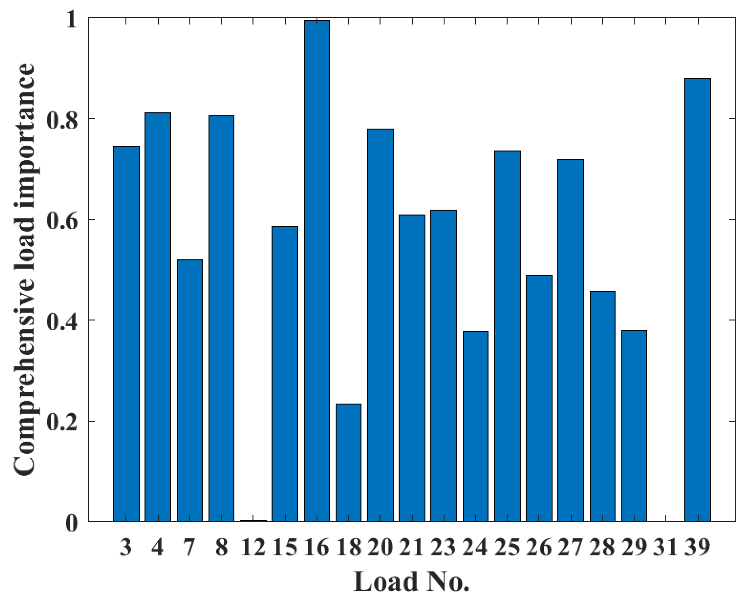
4.1. Load Importance Assessment

The system of IEEE39 nodes is used for the arithmetic analysis, and the system must be modified. Assuming each load node in the system represents an area with various electrical energy users inside, nodes 7, 16, 20, 26, 27, 28, and 39 contain typical industrial adjustable loads. Nodes 3 and 27 contain pharmaceutical companies. Nodes 7, 21, 23, and 25 contain semiconductor companies, with each node having 20 users inside. The following results can be obtained by the above-mentioned index calculation method, as shown in

Table 1. Table of load importance assessment index values.

Load No.	Load Topology Factor	Load Outage Loss	Load Regulation Capacity
3	0.702	3646.572	3.210
4	0.700	6558.973	5.412
7	0.325	5253.125	3.732
8	0.489	8684.986	9.490
12	0.354	103.588	0.120
15	0.589	4123.819	5.252
16	1	2913.223	16.291
18	0.569	3501.365	2.200
20	0.476	9633.306	6.292
21	0.539	3349.172	1.152
23	0.508	2946.491	1.444
24	0.532	4225.990	4.313
25	0.636	3109.785	1.515
26	0.760	5753.872	2.914
27	0.494	6153.832	6.731
28	0.337	6062.701	17.938
29	0.479	3112.751	3.659
31	0.316	117.652	0.148
39	0.383	14,606.531	18.409

.

The importance of each load in the different importance assessment indicators can be derived from Table 1, and the results of each indicator are analyzed below.

As can be seen from Figure 4 and

Table 2. Outage loss index value and load power top ten table.

Rank	Top 10 Load Outage Losses	Top 10 Load Power Loads
1	39	39
2	20	20
3	21	8
4	8	4
5	7	16
6	27	3
7	23	15
8	4	24
9	25	29
10	3	27

, there is a strong correlation between the size of the outage loss indicator and the load power size. The general characteristic is that the higher the power of the load, the higher its outage loss. But the outage loss ranking of the nodes also varies due to the different users contained within each load and the different sensitivity to losing the same amount of power. The size determination of outage loss depends on the power size of the load itself, but it is also influenced by the type of users within the load. Loads containing special users, such as semiconductor or pharmaceutical companies, will have a relatively significant impact on the value of the outage loss index.

For the load regulation capacity index, the results of its load regulation capacity index are shown in Figure 5. The load regulation capacity of loads 7, 16, 20, 26, 27, 28, and 39 containing adjustable industrial enterprises is better relative to that of load power similar and without adjustable industrial enterprises.

The three indicators for load importance assessment have been calculated above, and the combined load importance is derived by the ideal solution method. The combined weighting method of AHP and CRITIC was used to derive the final weights shown in

Table 3. Indicator weighting table.

Indicator	Load Topology Factor	Load Outage Loss	Load Regulation Capacity
Combined weights	0.330	0.432	0.238

.

Table 4. Top 10 ranking table of load composite importance and each index.

Rank	Load Importance of This Paper	Top 10 Ranking of Importance of This Article	Top 10 Ranking of Importance in Ref. [5]	Top 10 Load Topology	Top 10 Load Outage Losses	Top 10 Load Regulation Capacity
1	1	16	16	16	39	39
2	0.875	39	25	26	20	28
3	0.810	4	21	25	21	16
4	0.802	8	4	3	8	8
5	0.772	20	3	4	7	27
6	0.741	3	26	23	27	20
7	0.735	25	29	29	23	4
8	0.715	27	39	20	4	15
9	0.615	23	23	21	25	24
10	0.608	21	20	24	3	7

presents the top 10 loads ranked by their comprehensive load importance in this paper. Figure 6 and Table 4 demonstrate that the comprehensive load importance considers both the topological and electrical characteristics of the loads. Interestingly, 7 out of the top 10 nodes in the comprehensive load importance (nodes 3, 4, 16, 20, 21, 23, and 25) also appear in the top 10 of the agglomeration coefficient index. However, despite these 7 loads remaining in the top 10, their rankings differ when compared to each other. There are changes in the rankings. For instance, load 4 surpasses load 3 in ranking because of its higher value of the outage loss index. Conversely, load 25 drops in ranking due to its less prominent outage loss index and load regulation capability index. Additionally, some loads are more centrally located but do not contain special enterprises like semiconductors and have relatively lower load power. Despite this, their comprehensive importance still ranks them within the top ten, such as nodes 26, 29, and 24. It can be shown that the larger the agglomeration coefficient, the more centrally located the load is and, generally, the higher the importance, but its comprehensive importance is also influenced by the outage loss and load regulation capacity indexes.

In summary, the load importance assessment method considers the location characteristics of the node, the load’s sensitivity to outages, and its ability to enhance grid coordination. It treats the load as a zone, taking into account the types of users within the zone. The method calculates outage losses for the entire load zone, considering the varying outage sensitivity of different users. This comprehensive approach is more realistic than solely assessing based on load power, as it considers multiple factors that influence the importance of the load in the power system. Protecting critical loads based on the load criticality assessment method can minimize the damage after a sudden failure.

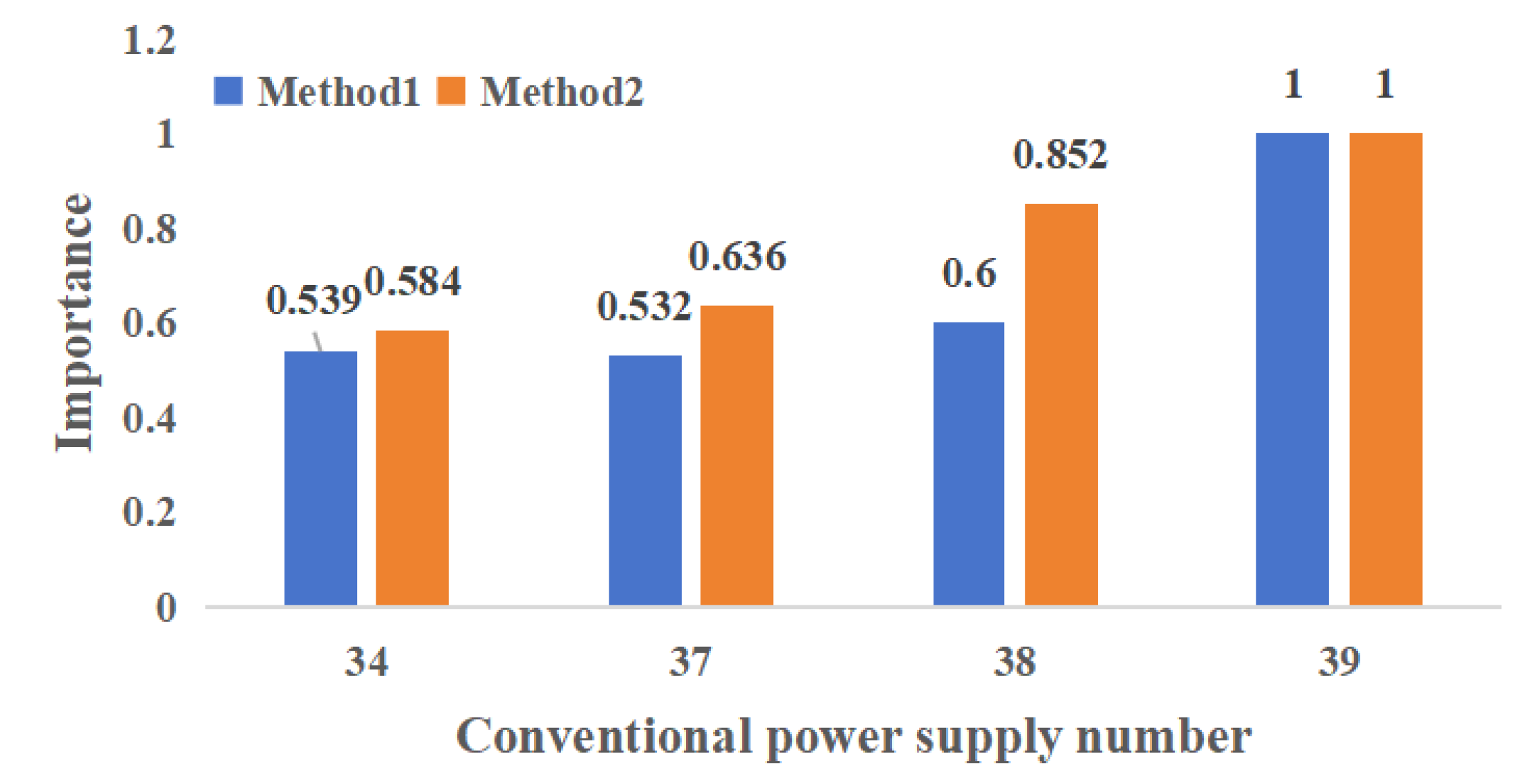
4.2. Power Supply Importance Assessment

Replacing some of the generators in the IEEE-39 system with new energy sources, the modified IEEE-39 system contains three wind farms and two PV farms. The wind farms are set in nodes 30, 32, and 33, and the PV farms are set in nodes 35 and 36. Using the historical wind speed data of wind farms and the historical light intensity data of PV farms in 2012 in a certain place, three of the wind farms and the sample data of two PV farms were taken.

Table 5. New energy parameter table.

Power No.	Type	Rated Capacity
30	Wind	250
32	Wind	650
33	Wind	632
35	Solar	650
36	Solar	560

and

Table 6. General power parameter table.

Power No.	Minimum Technical Output	Rated Capacity	Climb Rate
31	400	1100	350
34	158	508	200
37	150	540	225
38	430	830	300
39	500	1000	325

below present the parameter tables for new and conventional power sources, respectively, while Figure 7 represents the wind speed and light variation graphs for wind farms and PV plants.

In the context of the new energy scenario, the wind speed of the wind farm and the light intensity of the PV plant were used as input. The three-point estimation method was applied to obtain three estimation points for both wind speed and light intensity, as shown in

Table 7. Table of estimated wind speed and light intensity points for new energy fields.

New Energy Field	1	2	3	4	5
xi,1	13.91	13.51	15.81	1654.75	1437.21
xi,2	2.85	2.83	2.79	40.91	44.69
xi,3	8.65	8.06	9.25	464.67	462.61

.

To obtain the output data for the new energy field represented by each estimated point, 15 sets of tidal current input data were collected. Tidal current calculations were performed for each set, resulting in 15 sets of results. The weights assigned to each group are shown in

Table 8. Table of the weights of the results of the calculation of each group of currents.

Group	1	2	3	4	5	6	7	8	9	10	11
Weight	0.049	0.038	0.037	0.021	0.021	0.044	0.039	0.038	0.067	0.067	0.579

below.

The power distribution results of power supply loads obtained through the tide tracking method, combined with the load importance settlement results from Section 4.1, provide the comprehensive power supply coefficient of power supply and other indicators. Additionally, they show the importance results of various types of power supplies, as demonstrated in

Table 9. Conventional power supply index values and importance results.

Power No.	Combined Power Supply Actor	Maximum Spare Capacity	Climb Rate Coefficient	Conventional Power Importance	Importance of Substituting Power Supply Capacity for Integrated Power Supply Factor
34	390.984	350	0.394	0.539	0.584
37	361.583	390	0.417	0.532	0.636
38	418.569	400	0.361	0.6	0.852
39	873.018	500	0.325	1	1

,

Table 10. Wind farm values and importance results for each index.

Power No.	Combined Power Supply Factor	Equivalent Utilization Time Factor	Wind Farm Importance	Importance of Substituting Power Supply Capacity for Integrated Power Supply Factor
30	114.971	0.582	0.389	0.496
32	281.450	0.528	0.868	1
33	388.284	0.624	1	0.990

and

Table 11. Photovoltaic power plant index values and importance results.

Power No.	Combined Power Supply Factor	Equivalent Utilization Time Factor	PV Power Plant Importance	Importance of Substituting Power Supply Capacity for Integrated Power Supply Factor
35	111.563	0.356	0.734	1
36	137.167	0.362	1	0.742

, as well as Figure 8 and Figure 9. Method 1 in the figure is the evaluation method of power supply importance in this paper, and Method 2 is the evaluation method of replacing the comprehensive power supply coefficient with power supply capacity based on the method in this paper. The difference between the two methods is whether the influence of load importance is considered or not.

As observed from Table 9 and Figure 8, conventional power supplies 39 and 38 hold the first and second ranks in importance, mainly because of their high combined power supply factor and maximum standby capacity. On the other hand, power supplies 34 and 37, despite having relatively high climbing rate coefficients, cannot compensate for the gap in combined power supply factor and maximum standby capacity, leading to their lower ranks in importance.

The last column of Table 9 indicates the relative importance of conventional power supplies evaluated using Method 2. It can be found that the importance of power supply 37 is greater than that of power supply 34, and the overall relative importance of power supplies has increased. In Method 1, the reason why the importance of power supply 34 is higher than that of power supply 37 is that the main supply loads 20 and 16 of power supply 34 have higher importance compared to the main supply loads 25 and 3 of power supply 37. Consequently, despite power supply 37 having a higher rated capacity than power supply 34, its integrated supply factor is lower due to the difference in the importance of their main supply loads.

Correct, when load importance is not considered, the power supplied to different loads is treated equally. This means that there is no distinction between supplying power to important loads and supplying power to ordinary loads. Taking load importance into account is crucial to differentiate and prioritize the power supply to critical loads versus less critical loads, ensuring a more efficient and effective power distribution in the system.

From Table 10 and Table 11, and Figure 9, it is evident that the importance of new energy power supply is significantly related to its integrated power supply coefficient. However, when load importance is not considered, and the power supply capacity is used instead of the integrated power supply coefficient to assess the importance of power supply, the importance results of wind farms 32 and 33, and photovoltaic power plants 35 and 36 are exactly opposite to the results obtained using the method described in this paper. This highlights the significance of considering load importance in accurately assessing the importance of power supply from new energy sources. Exactly, although wind farm 32 has a higher capacity compared to wind farm 33, the main supply loads of wind farm 33 (loads 20 and 16) are more important than the main supply loads of wind farm 32 (loads 12 and 15). As a result, the integrated supply coefficient of wind farm 33 is higher than that of wind farm 32, especially when the difference in rated capacity between the two is not substantial. This illustrates the significance of considering load importance when evaluating the importance of power supply from different wind farms. Similarly, the difference in the importance of the two methods for photovoltaic power plants 35 and 36 is also due to the difference in the importance of the main supply loads of the two sources, with the importance of the main supply loads of the former 21 and 23 being lower than that of the main supply loads of the latter 23 and 24.

In a comprehensive comparison, the importance results of the power supplies obtained by considering the influence of load importance are different compared to those without considering. Considering the influence of load importance can reflect the importance of the power supplies supplying more important loads, and the resulting important power supplies can better guarantee the supply of important loads. Indeed, this research can be applied to enhance the power system’s resilience against disasters. By considering the importance of loads and power sources, a backbone network framework can be constructed, consisting of more crucial loads and important power sources, while minimizing the number of lines required. This approach focuses on protecting these critical components, aligning with the need to ensure continuous power supply to important loads and prevent chain failures from occurring. By implementing such a strategy, the power system’s ability to withstand disasters can be significantly improved.

5. Conclusions

This paper proposes a power source importance evaluation method based on load importance and new energy uncertainty. The method constructs a load importance evaluation system considering structural characteristics, outage loss, regulation capability, and other factors. To determine the importance of each load, the method uses the ideal solution method and ranks them accordingly. Next, the method calculates the power supply coefficient, which represents the power supply capability of the power source to the critical loads. This calculation involves using the three-point estimation method, which combines the characteristics of the new energy output and the importance of each load. Following that, the evaluation of load importance and the power supply capacity to critical loads is accomplished based on the ideal solution method, taking into account the diversity of power supply characteristics. This comprehensive evaluation allows us to assess the significance of each load and the power supply capability to meet the needs of critical loads, considering the unique characteristics of each power source. Finally, an example analysis is carried out on the IEEE39 to calculate the importance of various types of power sources, which can accurately reflect the power supply capacity of power sources to important loads and verify the validity of the evaluation method. The results of the example show the following:

(1)

The load importance assessment method takes a comprehensive approach, considering various factors such as the node’s location characteristics, the load’s sensitivity to power outages, and its ability to enhance the coordination capacity of the power grid. It treats the load as a part of the load area, accounting for the types of users within it and calculating the outage losses for the entire load area, considering the varying outage sensitivity of different users. This approach is more realistic than solely assessing based on load power. Additionally, the method also takes into account the adjustable ability of the load, highlighting the significant role of loads in participating in the coordination of the power grid source network.

(2)

The way of separately evaluating the importance of different kinds of power supply can fully evaluate the importance of power supply from the perspective of power supply and the characteristics of the power supply itself. Considering the influence of load importance and taking the comprehensive power supply coefficient as the assessment index, it can be concluded that the important power supply is more capable of guaranteeing the power supply of important loads.

(3)

This method plays an important role in the safe and stable operation of the power system. At the system network planning level, the load importance assessment helps construct a backbone network framework that prioritizes crucial loads and essential power sources while minimizing the number of lines required. By protecting this framework, we ensure the continuous power supply to important loads and reduce the risk of chain failures. This approach aligns with the objective of safeguarding the power system’s stability and resilience, thereby enhancing its ability to withstand potential disruptions and maintain a reliable power supply to critical loads.

References

1. Chao, Y.; Heyang, S.; Tong, L. Coupled Model and Node Importance Evaluation of Electric Power Cyber-Physical Systems Considering Carbon Power Flow. Energies 2022, 15, 8223. [Google Scholar] [CrossRef]
2. Wang, Y.; Zou, Y.; Huang, L.; Li, K. Key Nodes Identification of Power Grid Considering Local and Global Characteristics. Chin. J. Comput. Phys. 2018, 35, 119–126. [Google Scholar]
3. Geng, J.Q.; Piao, X.F.; Qu, Y.B.; Song, H.H. Method for Finding the Important Nodes of an Electrical Power System Based on Weighted-SALSA Algorithm. IET Gener. Transm. Distrib. 2019, 13, 4933–4941. [Google Scholar] [CrossRef]
4. Zou, Y.; Tan, S.; Liu, X.; Zhang, S.; Li, H. Power GridBased on Subnet Partition Key Node Recognition. Comput. Phys. 2013. [Google Scholar]
5. Zhao, Y.; Han, C.; Lin, Z.; Yang, L.; Wang, L.; Huang, J. Optimization Strategy of Two-Stage Core Backbone Grid of Power System with Renewable Energy. Power Grid Technol. 2019, 43, 371–386. [Google Scholar]
6. Chen, B.; Wang, H.; Cao, X. Optimization of Load Recovery in Late Stage of Grid Reconstruction Considering Load Fuzzy Uncertainty: Automation of Electric Power Systems. Autom. Electr. Power Syst. 2016, 40, 6–12. [Google Scholar]
7. Chen, P. Elastic Load Resource Aggregation and Regulate Potential Forecast Model Research; North China Electric Power University: Beijing, China, 2021. [Google Scholar]
8. Anderson, J. North American Power Futures Trading Volume on Nodal Exchange Jumps in April. Platts Megawatt Dly. 2019, 24, 2–3. [Google Scholar]
9. Banner, K.M.; Irvine, K.M.; Rodhouse, T.J. Statistical Power of Dynamic Occupancy Models to Identify Temporal Change: Informing the North American Bat Monitoring Program. Ecol. Indic. 2019, 105, 166–176. [Google Scholar] [CrossRef]
10. Chen, Q. The Assessment of the Outage Cost of Customersand the Cost-Effective of the Reliability of Distribution Network; Northeastern University: Boston, MA, USA, 2015. [Google Scholar]
11. Wang, Y.; Zhou, X.; Liu, H.; Chen, X.; Yan, Z.; Li, D.; Liu, C.; Wang, J. Evaluation of the Maturity of Urban Energy Internet Development Based on AHP-Entropy Weight Method and Improved TOPSIS. Energies 2023, 16, 5151. [Google Scholar] [CrossRef]
12. Lin, G.; Mo, T.; Ye, X. Critical Node Identification of Power Networks Based on TOPSIS and CRITIC Methods. High Volt. Eng. 2018, 44, 3383–3389. [Google Scholar]
13. Chen, C.; Rong, Y.; Ji, C. Speaker Verification Method Based on Deep Information Divergence Maximization. J. Commun. 2021, 42, 231–237. [Google Scholar]
14. Wang, W.; Chen, K.; Bai, Y. Comparative Study on Wind Speed Distribution Models of Hohhot Suburb Based on Measured Data. Acta Energ. Solaris Sin. 2021, 42, 370–376. [Google Scholar]
15. Fernandez-Jimenez, L.A.; Monteiro, C.; Ramirez-Rosado, I.J. Short-Term Probabilistic Forecasting Models Using Beta Distributions for Photovoltaic Plants. Energy Rep. 2023, 9, 495–502. [Google Scholar] [CrossRef]
16. Cheng, Z.-L.; Li, H.-K.; Li, F.-J.; Zeng, X.-Z. Multi Objective Optimal Power Flow Based on Wind Power Photovoltage Output Uncertainty. Control Theory Appl. 2021, 40, 11–16. [Google Scholar]
17. Xiao, Q.; Wu, L.; Chen, C. Probabilistic Power Flow Computation Using Nested Point Estimate Method. IET Gener. Transm. Distrib. 2021, 16, 1064–1082. [Google Scholar] [CrossRef]
Figure 1. Load importance ideal solution flow chart.
Sustainability 15 12941 g001
Figure 2. Flow chart of tide calculation based on point estimation method.
Sustainability 15 12941 g002
Figure 3. Flow chart of source importance evaluation based on ideal solution method.
Sustainability 15 12941 g003
Figure 4. Outage loss index value versus load power.
Sustainability 15 12941 g004
Figure 5. Load regulation capacity index chart.
Sustainability 15 12941 g005
Figure 6. Integrated load importance chart.
Sustainability 15 12941 g006
Figure 7. Variation curves of light intensity in part of photovoltaic power plant and wind speed in part of wind farm. (a) Variation curves of light intensity in part of photovoltaic power plant; (b) Variation curves of wind speed in part of wind farm.
Sustainability 15 12941 g007
Figure 8. Conventional power supply relative importance results.
Sustainability 15 12941 g008
Figure 9. Wind farm photovoltaic power plant importance degree results. (a) Wind farm importance degree results. (b) Photovoltaic power plant importance degree results.
Sustainability 15 12941 g009