Triaxial Shear Analysis Using Discrete Element Methods for Sandy Soil with an Improved Flexible Membrane Boundary

Abstract

Exploring strain localization has substantial potential to significantly impact the disaster resilience and mitigation capabilities of infrastructure, thus influencing project sustainability. Consequently, the field of sustainable geotechnical engineering is progressively directing attention toward studying soil strain localization. This research focuses on triaxial testing to deepen our understanding of this phenomenon by applying discrete element methods, thereby fostering the advancement of sustainable geotechnical engineering practices. While rigid-wall-based discrete element triaxial tests have been extensively studied, using flexible boundaries in these tests has received limited attention. This study introduces a three-stage method to enhance stress application in flexible membranes by applying confining pressure. A comparison of triaxial tests was conducted at both macroscopic and microscopic scales, utilizing flexible and rigid boundaries. Moreover, numerical simulations were performed on flexible membrane samples with various particle sizes to identify appropriate dimensions for flexible boundaries. Our results demonstrate that the improved flexible membrane provides more accurate representations of macroscopic and microscopic sample variations than rigid walls. Keeping the particle sizes for flexible membranes within the range of 0.2 to 0.8 times the characteristic particle size (r) is essential for striking a balance between simulation accuracy and computational efficiency. These findings enhance the accuracy of triaxial compression test simulations and offer a valuable foundation for studying strain localization in soils. Understanding these phenomena is essential for various geotechnical engineering applications, such as foundation design and slope stability analysis. Furthermore, these findings form a pivotal foundation for resource optimization and enhancing the reliability of engineered structures, thereby driving the advancement of sustainable geotechnical engineering practices.

1. Introduction

Strain localization, a phenomenon characterized by the concentration of strains within specific spatial regions [1], is frequently linked to the degradation of geotechnical materials. Studying strain localization is pivotal in sustainable geotechnical engineering, as it directly influences the dependability and security of engineering structures and the effective utilization of resources. This phenomenon becomes apparent in various scenarios, such as practical situations involving shear-related degradation, like the sliding of embankment dams. Moreover, strain localization has been observed in experiments conducted with indoor soil samples [2,3,4,5,6,7,8,9]. The implications of strain localization can encompass failures, deformations, or even the collapse of infrastructure, thereby impacting the longevity and performance of projects. Shear zones are regions where strains intensify within confined spaces, forming formations that resemble strips. The formation and evolution of these shear zones exhibit distinct characteristics of strain localization, playing a crucial role in significantly influencing the mechanical properties of the soil mass [6,10,11].

Therefore, it is crucial to understand the mechanism governing shear zone formation and accurately depict this phenomenon [9,12]. This study can potentially improve infrastructure design, construction, and operational processes, thereby contributing to enhanced project sustainability. Many scholars have chosen indoor tests to observe shear zones due to their convenient execution [13,14,15,16]. However, these tests provide only a macroscopic perspective on soil shear damage, lacking the capacity to capture the intricate attributes of strain localization. Consequently, numerous researchers have turned to numerical simulation techniques. The finite element method has been widely used to simulate the development and progression of the shear zone [17,18,19,20,21,22]. However, limitations in the intrinsic model and continuum medium algorithm can result in significant mesh-related dependencies in the evolution of shear bands following strain localization.

Recent advancements in computational speed have facilitated innovative approaches to numerical simulation. The discrete element method, which considers particle interactions at a microscopic scale and incorporates parameters like particle size, shape, and gradation, enhances the accuracy of soil behavior simulations [23]. A focused study using the discrete element method is essential for precisely depicting shear zone development.

Researchers have utilized the discrete element method to investigate the developmental mechanism of shear bands. They have explored the formation mechanism and mechanical response of shear zones during biaxial tests [1,24] and direct shear tests [25]. Additionally, researchers have studied factors such as constraint pressure [26] and drainage-consolidation conditions [27] that influence strain localization. Nevertheless, several discrete element analyses have used rigid walls for simplicity [28,29], which restrict lateral deformation and may introduce discrepancies.

In response to this challenge, flexible membranes have increasingly been used to analyze mechanical responses. Initially, particles located at the specimen’s periphery were used as flexible membranes to assess the compatibility of the discrete element model with indoor tests and to examine micro-level changes within the sample [30]. However, this approach introduced an inconsistency: particles could be classified as specimen particles in one computational cycle and membrane particles in the next, requiring consistency in material properties. To overcome this limitation, hexagonal spherical particles were introduced as constituents for constructing flexible membranes. This allowed the separate assignment of material properties from those of specimen particles [31]. Nevertheless, despite this improvement, the movement of membrane particles continued to be constrained in the X and Y directions, although they could move along their respective layers.

In this regard, Lu et al. [32] introduced a novel method that employs a quadrilateral arrangement of spherical particles in constructing flexible membranes. They emphasized the importance of maintaining a greater height for the flexible membrane than the specimen to achieve uniform force distribution at both ends [32]. Qu et al. [33] extended this approach by utilizing strain energy equivalents in constructing flexible membranes and conducting a comparative analysis of triaxial tests involving flexible and rigid boundaries. Numerous researchers have also investigated the mechanical behavior of specimens with flexible membrane boundaries [34,35,36,37,38].

These membranes exhibit noticeable evolution, transitioning from an initial roughness to gradual refinement. In the initial stages, rough peripheral particles were utilized, and then, transitioned to a compact hexagonal arrangement. Subsequently, an approach considering the mechanical behavior of the top and bottom edges was introduced, leading to an increased membrane height. Research suggests a correlation between the application of confining pressure and simulation accuracy [31,39]. Furthermore, the constituent membrane particle size significantly impacts the behavior, computational accuracy, and efficiency of triaxial samples [40]. Therefore, particle size selection plays a critical role in constructing these flexible membranes.

However, it is essential to note that the primary methods of applying force to flexible membranes include the single-force and two-stage force modes. Nevertheless, the single-force mode is susceptible to soil particle overflow from the gap between the flexible membrane and the loading plate. On the other hand, the two-stage force mode restricts particle movement in the X–Y plane of both the upper and lower flexible membranes, resulting in an uneven stress distribution across the specimen. Moreover, the current research on determining the particle size of the constituent flexible membranes is limited, lacking a solid scientific foundation for making informed membrane selections. The accurate choice of membrane particle size and the appropriate application of flexible boundary confining pressure directly influence simulation precision, thereby contributing to the scientific understanding of shear zone development.

To address the current research gap in membrane particle size selection and boundary confining pressure application, this paper utilizes the PFC3D 5.0 software. To improve the rationale for applying confining pressure to specimens, refinement is introduced to the methodology of applying confining pressure. This refinement proposes a three-stage approach for applying confining pressure. This method involves using three distinct confining pressures: at the specimen’s location, on top of the specimen, and at the flexible membrane higher than the specimen. Subsequently, numerical simulations of triaxial tests are conducted on specimens with a flexible membrane and are compared with specimens using rigid walls. This comparative analysis covers both the macroscopic and microscopic scales of investigation.

Additionally, diverse particle sizes are chosen to form flexible membranes. These membranes undergo triaxial tests using specimens incorporating flexible membranes with varying particle sizes. This comparative investigation is performed on a macroscopic scale.

The primary objective of this study is to determine the optimal methods for applying confining pressure and determining suitable particle sizes for flexible membranes. These findings are expected to contribute significantly to our shear zone development comprehension.

In summary, this research aims to provide insights into the application of confining pressure and the selection of particle sizes for flexible membranes. These contributions aim to enhance the understanding of the mechanisms underlying shear band development. The results of this study can serve as a fundamental reference for integrating flexible membranes into triaxial tests, facilitating their broad application in investigations related to strain localization. By thoughtfully considering these localization phenomena, we can optimize the utilization of natural resources, minimize environmental impacts, and ensure the enduring sustainability of engineering.

2. Materials and Methods

This study utilized the Particle Flow Code in Three Dimensions (PFC3D) software, developed by Itasca, to investigate suitable methods for applying confining pressure and determining the optimal size of the flexible membrane particles. This software’s selection aligns precisely with this paper’s research objectives. To ensure comparability with the indoor tests, as recommended by Li et al., the numerical simulation used specimens with dimensions similar to those in the indoor tests. Therefore, a cylindrical specimen was chosen to simulate the indoor triaxial test, with sizes that precisely match those of the indoor test specimen (diameter of 40 mm and height of 80 mm). Detailed explanations of soil specimen preparation, the generation of boundary conditions, parameter selection, and data acquisition are provided in the following sections.

2.1. Establishment of Flexible Boundaries

In indoor triaxial tests, latex membranes possess notable qualities characterized by their high flexibility and strong tensile properties, referred to as flexible boundaries [32]. However, creating flexible boundaries in three dimensions poses a challenge, which has led to the prevalent use of rigid walls in simulations instead of latex membranes. Qu et al. [33] noted that rigid walls impede strain localization within the specimen, possibly leading to inaccurate estimations of specimen strength. Furthermore, rigid walls fundamentally contrast with the flexible characteristics of latex membrane boundaries.

Cil et al. [34] demonstrated that flexible membranes, formed by assembling discrete particles, can be stretched and contracted similarly to latex membranes. This property enables them to replicate the flexible characteristics of latex membranes in the context of discrete element method (DEM) simulations. Consequently, in this study, a flexible membrane formed by combining spherical particles acts as an approximate substitute for the latex membrane in indoor tests.

Considering the current approach to establishing the flexible membrane and the loading mechanism, a three-stage method is proposed for applying the confining pressure. The steps in this modeling approach include determining the particle size of the boundary particles, identifying particle generation positions, establishing the contact model, and applying pressure to these boundary particles.

2.1.1. Determination of Boundary Particle Size

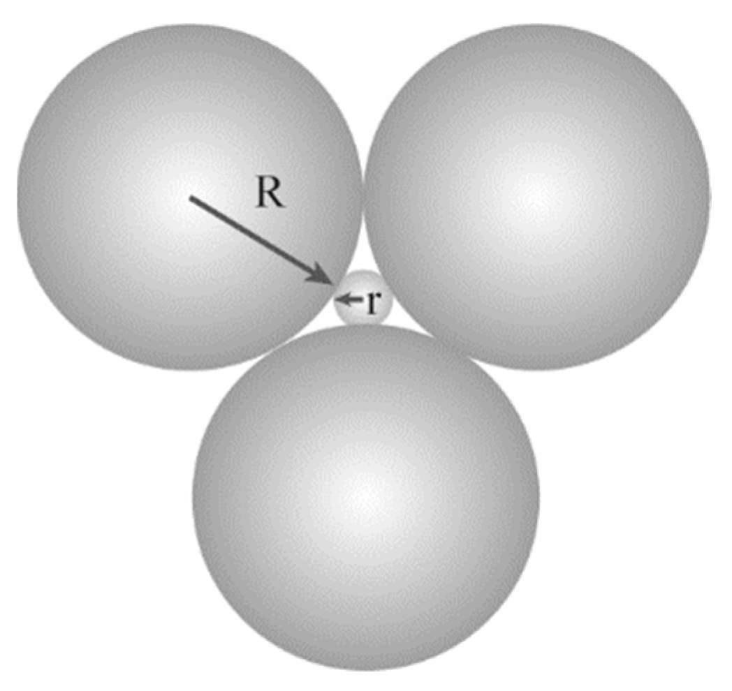
The particles used in the flexible boundary have identical diameters, and their size corresponds to the particles within the soil specimen [35]. Lu et al. [32] highlight these membrane particles’ role in facilitating the specimen’s local deformation while applying confining pressure to the soil particles. Despite the difference in diameter between the flexible membrane particles used in the numerical triaxial simulation test and the thickness of the latex membrane in the indoor triaxial test, it is sufficient if they exhibit similar tensile properties and ensure a reasonable application of confining pressure. As shown in Figure 1, the maximum allowable size of the flexible membrane particles in the simulation can be determined by Equation (1) and the equation can ensure that the smallest soil sample particles do not escape through the boundary gaps.

Although a smaller flexible membrane particle size is theoretically more ideal for applying peripheral pressure to the sample, excessively small particles can substantially increase computation time. Consequently, Lu et al. [32] chose a particle size of 2.8 mm to create a flexible membrane, resulting in a ratio of 25 between the sample width and the flexible membrane particle size. Based on this size and considering computational efficiency, this paper presents a method for setting up a flexible membrane, using a 1 mm radius for the boundary particles.

$$R\le 3/(2\sqrt{3}-3)r$$

(1)

In Equation (1), R (m) is the radius of the flexible film particles, and r (m) is the radius of the specimen particles.

2.1.2. Determination of the Location of the Generation of Each Particle at the Boundary

Previous studies conducted by scholars have investigated the arrangement of particles in the flexible membrane and have determined that a hexagonal layout is more appropriate. This layout ensures that each membrane particle is surrounded by six neighboring particles, which better reflects the continuity of the flexible membrane [38]. Hence, this paper adopts the hexagonal layout for modeling the flexible membranes using spherical particles.

For the triaxial numerical simulation test, the size of the specimen was 40 mm × 80 mm. A total of 46 layers of spherical particles were generated along the z-axis direction, from top to bottom, with each layer comprising 63 spherical particles. Figure 2 presents a schematic diagram illustrating the modeling of the flexible membrane.

To enhance the establishment of the flexible membrane model, an improvement was made based on the research conducted by other scholars [26]. In this improvement, two additional layers of spherical particles were generated at the upper and lower ends of the model. These four layers of spherical particles were fixed in place to simulate the function of an O-ring. This addition stabilizes the specimen during the confining pressure servo or shear process. It prevents the internal particles from spilling beyond the loading wall and the boundary particles within the gaps.

Furthermore, a separate confining pressure was applied to the flexible membrane near the loading plates to ensure the rationality of the forces acting on the specimen at the upper and lower loading plates.

As a result of these modifications, the final size approximation of the flexible membrane model is 40 mm × 87 mm × 2 mm (diameter × height × thickness).

2.1.3. Selection of a Contact Model between Boundary Particles

The representation of flexibility in flexible membranes plays a significant role in model calibration, and it primarily relies on the contact bonding behavior between the constituent particles of the flexible membrane. Hence, selecting an appropriate interparticle contact model is crucial to simulate flexible membranes accurately.

In indoor experiments, the latex membrane typically undergoes tensile deformation. Considering the similarities between the mechanical properties of the latex membrane’s tensile deformation and the “linear bonding contact model” in PFC3D within the bond strength range, this paper chooses the “linear bonding contact model” as the contact model for the membrane particles. This selection ensures that the mechanical properties of the contact model align well with the tensile deformation behavior of the latex membrane. This model selection aligns with the contact model used in the study by Qu et al. [33]. The parameters for the contact model were derived from numerical tensile tests performed on the flexible boundary. The calibrated results of this process are visually presented in Figure 3.

2.1.4. Application of Boundary Particle Confining Pressure

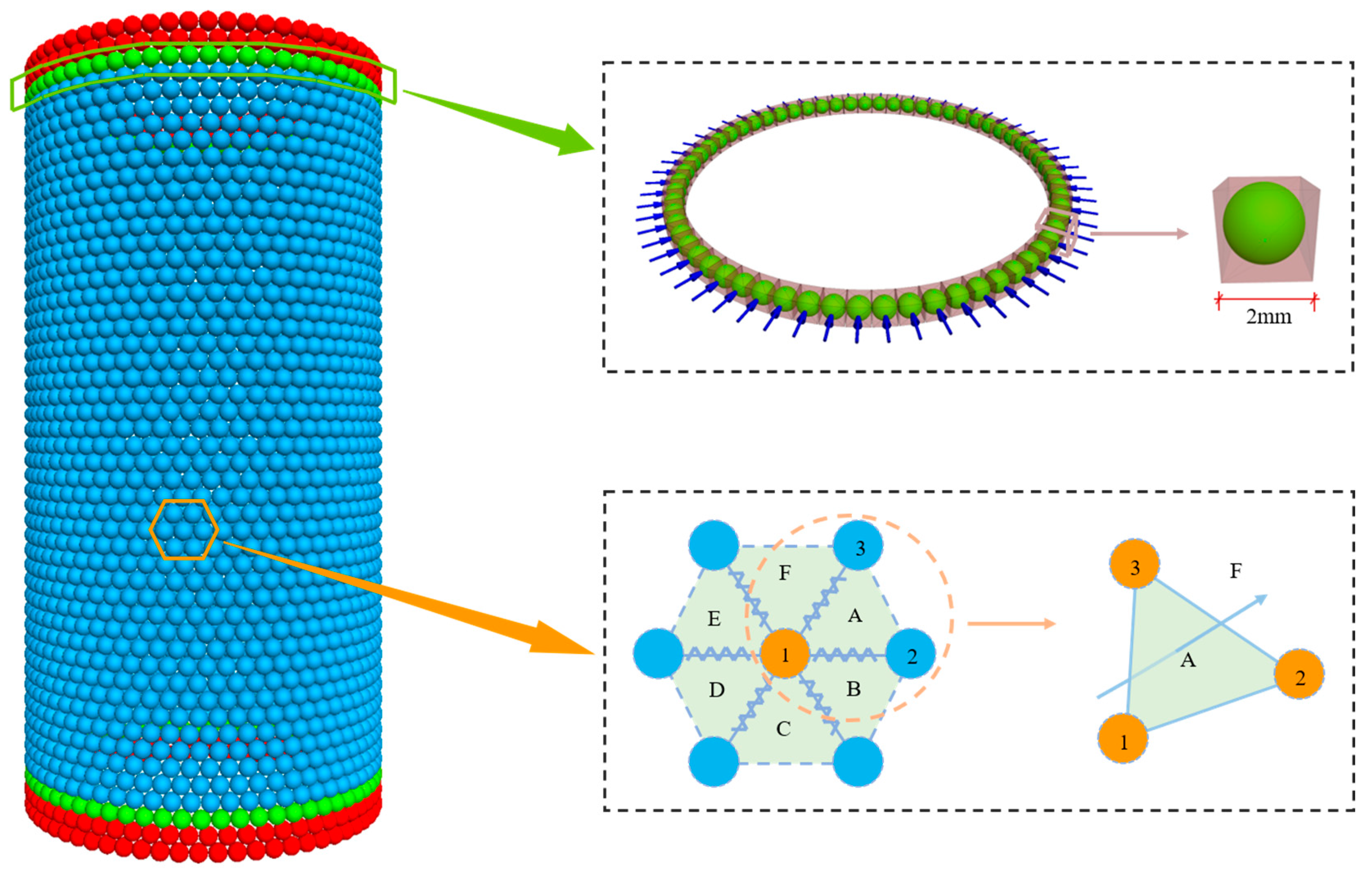
To ensure a more realistic application of confining pressure to the specimen, this paper classifies the flexible membrane into three groups: boundary group 1, comprising the upper and lower edges indicated by the red particles; boundary group 2, composed of the green particles near the upper and lower loading plates; and group 3, representing the central section of the flexible membrane’s main body and depicted by the blue particles. The grouping diagram can be found in Figure 4.

For each group of the flexible membranes, different algorithms were utilized to apply the confining pressure:

• Boundary Group 1 Confining Pressure Setting

Boundary group 1 prevents specimen shaking and particle spillage at the upper and lower boundaries during the simulation. To replicate the function of an O-ring in indoor triaxial tests, boundary group 1 remains fixed throughout the simulation.

2.

Boundary Group 2 Confining Pressure Setting

Circumferential pressure is applied to Boundary Group 2, where each ball particle is modeled as a cube externally tangent to the ball. Boundary Group 2 comprises the portion of the specimen in contact with the loading plate. According to Wang [41], the specimen’s end-boundary conditions significantly influence the shear zone’s development. Previous studies have constrained the movement of the specimen’s ends in the X–Y direction. This paper applies confining pressure specifically to the particles within Boundary Group 2 to accurately simulate indoor testing conditions, as illustrated in Figure 4. The force acting on these particles is computed using Equation (2):

$$\overrightarrow{F}={\sigma }_3\times L^2\times {\overrightarrow{n}}_r$$

(2)

where $\overrightarrow{F}$ (KN) is the vector force applied to the center of each particle in boundary group 2, $L$ (m) is the length of a side of a cube, ${\sigma }_3$ (kPa) is the confining pressure, and ${\overrightarrow{n}}_r$ is the unit vector, with the center of each spherical particle pointing to the center of the circle in which the boundary group 2 is located.

3.

Boundary Group 3 Confining Pressure Setting

To accurately apply the confining pressure to the specimen even during the deformation process, the method proposed by Z. Li [33] is utilized for setting the confining pressure on the particles of boundary group 3. The external force applied to the boundary group 3 particles is calculated using the following equations:

$$\overrightarrow{F}={\sigma }_3\times A^{123}\times {\overrightarrow{n}}^{123}$$

(3)

$${\overrightarrow{F}}_{1A}={\overrightarrow{F}}_{2A}={\overrightarrow{F}}_{3A}=\frac{1}{3}\times ‖F‖\times {\overrightarrow{n}}^{123}$$

(4)

$${\overrightarrow{F}}_1={\overrightarrow{F}}_{1A}+{\overrightarrow{F}}_{1B}+{\overrightarrow{F}}_{1C}+{\overrightarrow{F}}_{1D}+{\overrightarrow{F}}_{1E}+{\overrightarrow{F}}_{1F}$$

(5)

where ${\sigma }_3$ (kPa) is the confining pressure, $A^{123}$ is the area of triangular unit plane 123, and ${\overrightarrow{n}}^{123}$ is the unit normal vector of the triangle face.

2.2. Sample Preparation

The experiment employed on-site sandy soil with a dry density of 1.66 g/cm³ and water content of 8%, in accordance with the soil sample gradation depicted in Figure 5. Unconsolidated and undrained tests were conducted using GDS static triaxial apparatus, standard equipment for such experiments. Previous research by Zhou [42] and colleagues indicates that when the shear rate in the triaxial shear test remains at or below 0.10 mm/min, the shear strength of sandy soil shows limited discernible variations under different effective confining pressure conditions. Consequently, the test loading rate was set at 0.1 mm/min. The results of the indoor testing are illustrated in Figure 6.

Spherical particles were used in the indoor triaxial test simulation to represent the constituent particles of the specimens. The efficiency of computer operations is essential during the soil specimen generation process. Directly using the indoor sand and soil gradation for numerical simulation would decrease computational efficiency, considering the fine nature of the indoor test sand and soil particles. To address this, in this paper, the gradation range was expanded five times while maintaining the accuracy of the calculation results. The selection of the particle gradation model is depicted in Figure 5. A total of 7045 particles were generated, a quantity considered sufficient for achieving stable computational results, as demonstrated by Kuhn and Bagi [43].

Moreover, considering the presence of rolling resistance during the shear process of sand particles, the selected contact model for the sand particles was the anti-rolling linear contact model. The initial porosity ratio of the numerical specimens was set at 0.389, which is consistent with the conditions in the indoor experiments. Confining pressures of 50 kPa, 100 kPa, and 150 kPa were selected based on the isotropic compression approach used in the studies by Lu [32], Cil [34], and other researchers. To achieve quasi-static conditions and loading efficiency [33], the loading plate was adjusted at a rate of 5 mm/s. The calibration method proposed by Cil [34] was employed to calibrate the stress–strain behavior of numerical specimens with that observed in indoor experiments. Figure 6 illustrates the calibration process results, visually representing the aligned stress–strain behavior. The calibrated parameters are provided in

Table 1. Meso-parameters of the particle contact.

Microscopic Parameters	Kn/Ks	Friction	cb_Tenf	cb_Shearf	rr_Fric
Flexible boundary	1	0	5 × 1010	5 × 1010	0
Soil particles	3	0.4	/	/	0.5

.

Two setups were analyzed to assess the impacts of different boundary conditions on the simulation outcomes: one with a flexible membrane and another with a rigid wall. The particle size for the flexible membrane was specifically set at 0.75 mm through preliminary calculations to ensure precise data generation. The Fish function in the software was employed to directly extract stress–strain data, which were then presented as stress–strain curves. A qualitative assessment was carried out by comparing these curves from both setups with the experimental data, as confirmed in previous studies [32,33,34]. Porosity data were obtained using measuring spheres with a radius of 4 mm and exported through the Fish language. A porosity cloud, visualized from this measured data, facilitated the observation of porosity changes during shear zone evolution [1,26]. Through this qualitative analysis, it was possible to track the development of the shear zone alongside changes in the porosity distribution.

The impact of particle size on the simulation results was explored by examining seven different particle sizes. By analyzing stress–strain cloud diagrams derived from these sizes and comparing them with the experimental curves, the appropriate particle size for the flexible membrane was determined.

This paper primarily analyzes porosity and coordination number data to elucidate the mechanism behind shear zone development characteristics. Also, measurement circles were established inside and outside the shear zone, and stress–strain curves within these zones were analyzed qualitatively. Porosity, coordination number, and stress–strain data were obtained using the Fish language in PFC3D.

However, it is essential to note that isotropic consolidation in this study may not be universally applicable to all engineering scenarios due to specific soil conditions or other factors.

This section describes the sample parameters required for the tests, simulations, and data acquisition. The following section will delve into the impacts of the flexible membranes on the simulation results and the shear behavior of sandy soils.

3. Results

3.1. Comparative Analysis of the Effect of Latex Film on the Simulation Results

Figure 6 displays the stress–strain curves obtained from the simulations, highlighting variations under different boundary conditions. The evolution of the shear zone was monitored through porosity analysis. A monitoring point approach was employed due to software limitations preventing cloud diagram export. Figure 7 illustrates the arrangement of the monitoring points, while Figure 8 displays the resulting porosity distribution map.

Upon comparing the stress–strain curves obtained under different confining pressures, several noteworthy observations can be made. Firstly, at a confining pressure of 50 kPa, the proportional limit point of the stress–strain curve obtained from the simulation using the flexible membrane setup closely matches the proportional limit point of the test curve. In contrast, the proportional limit point of the stress–strain curve obtained from the simulation using the rigid wall setup significantly differs from the test curve.

Additionally, the peak stress point in the stress–strain curve from the simulation with the flexible membrane setup is slightly higher than that of the test curve. Conversely, the peak stress point in the stress–strain curve from the simulation with the rigid wall setup is noticeably lower than that of the test curve.

With increasing confining pressure, the stress–strain curve from the simulation using the flexible membrane setup shows improved agreement with the test curve. The proportional limit point and the peak stress point of these two curves almost coincide. In contrast, the corresponding points in the stress–strain curve obtained from the simulation using the rigid wall setup remain significantly different from those in the test curve.

Using a flexible membrane in the simulation greatly enhanced the predictions for the proportional limit and the peak stress of the granular material. Compared to the simulations with a rigid wall at a 150 kPa confining pressure, using a flexible membrane improved predictions by 9.4% for the proportional limit and 5.3% for the peak stress. This indicates that specimens with flexible membranes offer a more accurate representation of stress–strain behavior.

Lu et al. [32] noted that applying rigid constraints in simulations can cause localized zones of damage and lead to excessive confining pressures. This, in turn, may lead to inaccuracies in predicting post-peak behaviors. Thus, utilizing a flexible membrane to obtain stress–strain curves for the specimens provides a more reasonable and accurate representation of their mechanical response.

The porosity cloud plots obtained from the simulations with different boundary conditions offer valuable insights into specimen behavior. A comparison of the results shows that using a flexible membrane to simulate the latex membrane enables the clear monitoring of compression zone generation and shear band development at both ends. In contrast, these phenomena are not clearly observed in the simulation using a rigid wall.

The differences in observations arise from the limitations of the rigid wall setup, which solely permits overall lateral deformation, lacking the ability to accommodate bulge deformation. In contrast, the flexible membrane, consisting of pebble combination particles simulating the latex membrane, can induce bulge deformation that better matches the actual behavior of the specimen. Moreover, the flexible membrane setup allows for the unrestricted relative movement of particles within the specimen, providing a representation that aligns more closely with the conditions encountered in indoor model tests.

As a result, selecting the flexible membrane to simulate the latex membrane yields a more accurate prediction of the macroscopic stress–strain behavior and deformation characteristics of granular materials.

Applying confining pressure to a sample using a flexible film involves exerting force on the particles that make up the film. Thus, the size of these particles directly affects the effectiveness of applying confining pressure to the sample, thereby influencing the simulation’s accuracy. To address this issue, seven schemes are employed for generating flexible membranes, each with different particle radii: 2.5 mm (R/r = 2), 1.875 mm (R/r = 1.5), 1.25 mm (R/r = 1), 1 mm (R/r = 0.8), 0.75 mm (R/r = 0.6), 0.5 mm (R/r = 0.4), and 0.25 mm (R/r = 0.2). R represents the flexible membrane’s particle radius, and r corresponds to the minimum particle size in the group with the widest particle size range within the sample. Notably, the discrepancy between the confining pressure ultimately applied to the sample and the predetermined confining pressure is kept within 5%. Figure 9 displays the stress–strain curve obtained from the simulation.

Figure 9 clearly illustrates the influence of confining pressure and radius ratio on the simulation results. For a confining pressure of 50 kPa and a radius ratio greater than or equal to 1, the simulation curve consistently lies below the corresponding test curve, showing significant deviations at both the proportional limit and peak stress points. In contrast, for a radius ratio of less than 1, the simulation curve tends to lie above the test curve, closely matching it at the proportional limit point but slightly surpassing it at the peak stress point. Furthermore, as the confining pressure increases to 100 kPa and 150 kPa, discrepancies between the simulation and test curves become evident, particularly in cases where the radius ratio is greater than or equal to 1, specifically at the peak stress point. In contrast, for cases where the radius ratio is less than 1, the simulation curves show excellent agreement with the test curves, with a satisfactory overlap observed at the proportional limit point.

In conclusion, when the radius ratio exceeds 0.8, the flexible membrane exhibits greater roughness, leading to more notable disparities between the simulated and actual results. Conversely, a radius ratio below 0.2 results in excess particles in the flexible membrane, leading to extended computation times and increased costs. Therefore, to strike a balance between accuracy and efficiency, keeping the radius ratio within the range of 0.2 to 0.8 is advisable.

In conclusion, an optimal radius ratio between 0.2 and 0.8 ensures a balanced trade-off between computational precision and efficiency. This finding contrasts with conclusions from other researchers. For instance, scholars like Qu et al. [33] stress the importance of accounting for boundary effects when choosing the particle size of the flexible membrane. On the other hand, researchers like Cil et al. [34] suggest using the smallest specimen particles as a reference. However, it is essential to acknowledge that the smallest particle size may vary among different test conditions. Relying solely on the smallest particle size as the criterion for selecting the size of the flexible membrane may result in inefficient computations. The flexible membrane functions as a conduit for transferring confining pressure, achieving this through interactions with the specimen particles, as indicated by Lu and other researchers [32]. A more rational approach involves selecting the flexible membrane’s size while considering the specimen particles’ dimensions.

3.2. Study of the Shear Mechanical Behavior of Sandy Soils

3.2.1. Macroscopic Mechanical Response

The research above demonstrates that using flexible membranes offers a more accurate representation of particles’ macroscopic behavior and deformation characteristics. Moreover, using flexible boundaries with a radius ratio ranging from 0.2 to 0.8 strikes a balance between calculation accuracy and efficiency. Based on these findings, a particle size of 0.75 mm is chosen for the flexible boundary to conduct a comprehensive investigation into the shear mechanical behavior of sand. 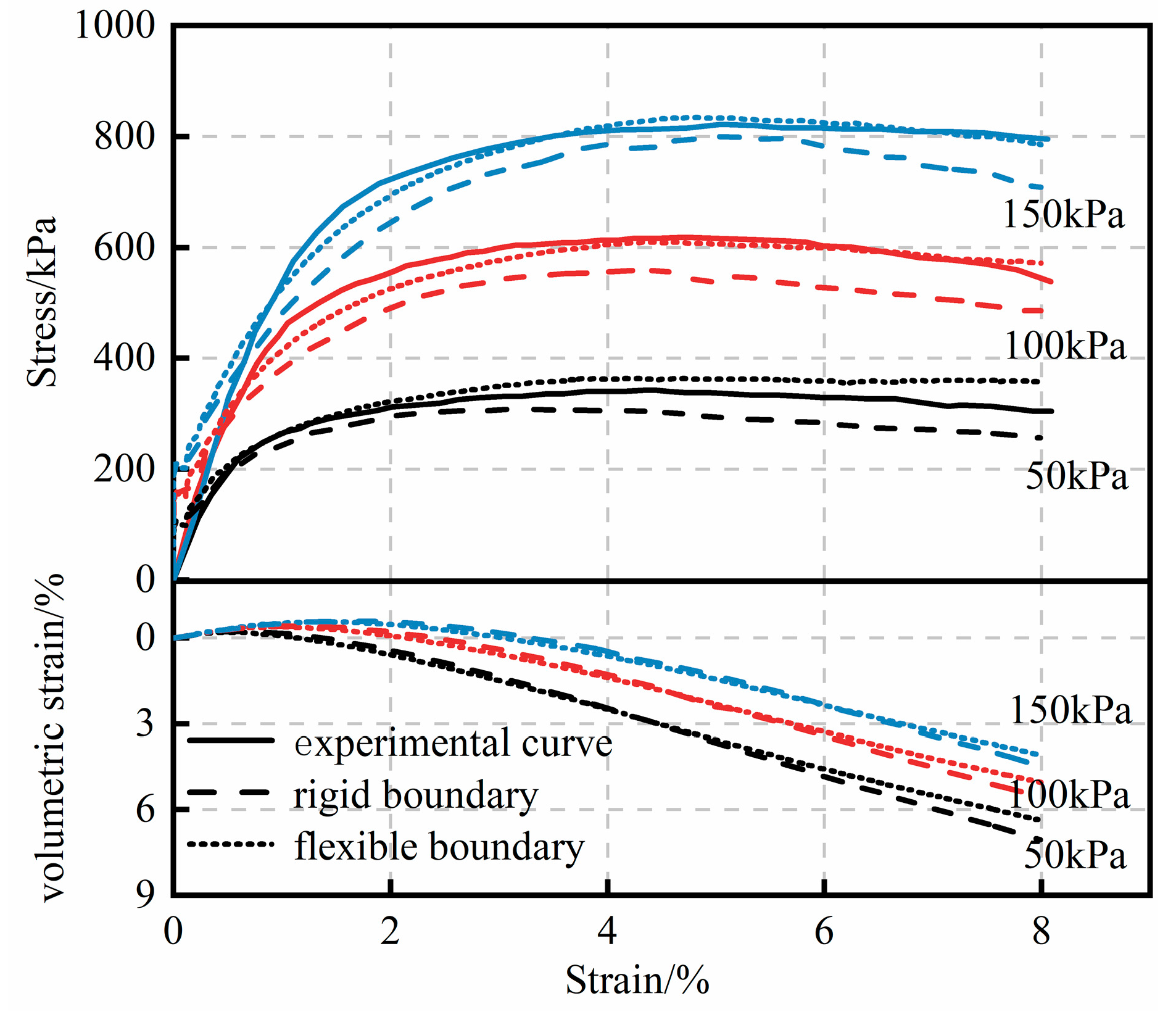Figure 10 displays the stress–strain and volume–strain curves obtained from the simulation. The volumetric strain during triaxial compression is calculated using Formula (6) in the programming. Additionally, the radial strain in the flexible boundary is determined by averaging the radial strain at each small ball position, which is calculated programmatically by traversing the small balls in the flexible boundary.

$$\theta =\frac{V^{\prime }-V}{V}= {\varepsilon }_h+ 2{\varepsilon }_r$$

(6)

where $\theta$ is the volumetric strain, ${\varepsilon }_h$ is the axial strain, and ${\varepsilon }_r$ is the radial strain.

From Figure 10, it is evident that the simulation results of samples with flexible membranes closely resemble the indoor experiments. In contrast, samples with rigid walls exhibit earlier entry into the strain-softening stage compared to both the indoor experiments and samples with flexible membranes. As volume–strain measurements were not conducted during the indoor investigations, the analysis solely concentrates on the volume–strain curve obtained from numerical simulation.

As depicted in the figure, the numerical simulations display volume shrinkage during the initial loading stage. The maximum volume shrinkage of the flexible membrane specimens under different confining pressures is similar to that of the rigid wall specimens. Subsequently, the samples begin to expand after reaching the peak of volume shrinkage. The volume expansion rates of samples with flexible membranes at the end of loading under different confining pressures are measured as 6.4%, 5.0%, and 4.1%. In comparison, samples with rigid walls exhibit rates of 7.1%, 5.6%, and 4.5%, respectively. It becomes clear that with increasing confining pressure, the difference in volume expansion between the two boundary conditions gradually diminishes, resulting in the convergence of the volume–strain curves for samples with rigid walls and samples with flexible membranes. This convergence can be attributed to the improved restraining capacity of the flexible membrane against the lateral deformation of the specimen under increasing confining pressures.

Consequently, the flexible membrane can be effectively considered a rigid wall at a sufficiently high confining pressure. However, the simulation of volume–strain by flexible membranes provides more detailed results, particularly in capturing the volume expansion behavior. This observation corroborates the findings of Lu et al. [32]. However, it is essential to note that their study primarily concentrated on simulations involving loose sand, whereas our research specifically examines the behavior of dense sand.

3.2.2. Porosity and Particle Coordination Number Distribution

The formation of the shear zone in the specimen involves alterations in both porosity and particle coordination number. This occurs due to the relative sliding of soil on both sides of the shear zone, resulting in heightened disturbance and the loosening of the soil structure within the shear zone. Consequently, this leads to an increase in porosity and a decrease in the coordination number of particles. By monitoring the changes in porosity and coordination number, valuable insights can be gained into the development of the shear zone.

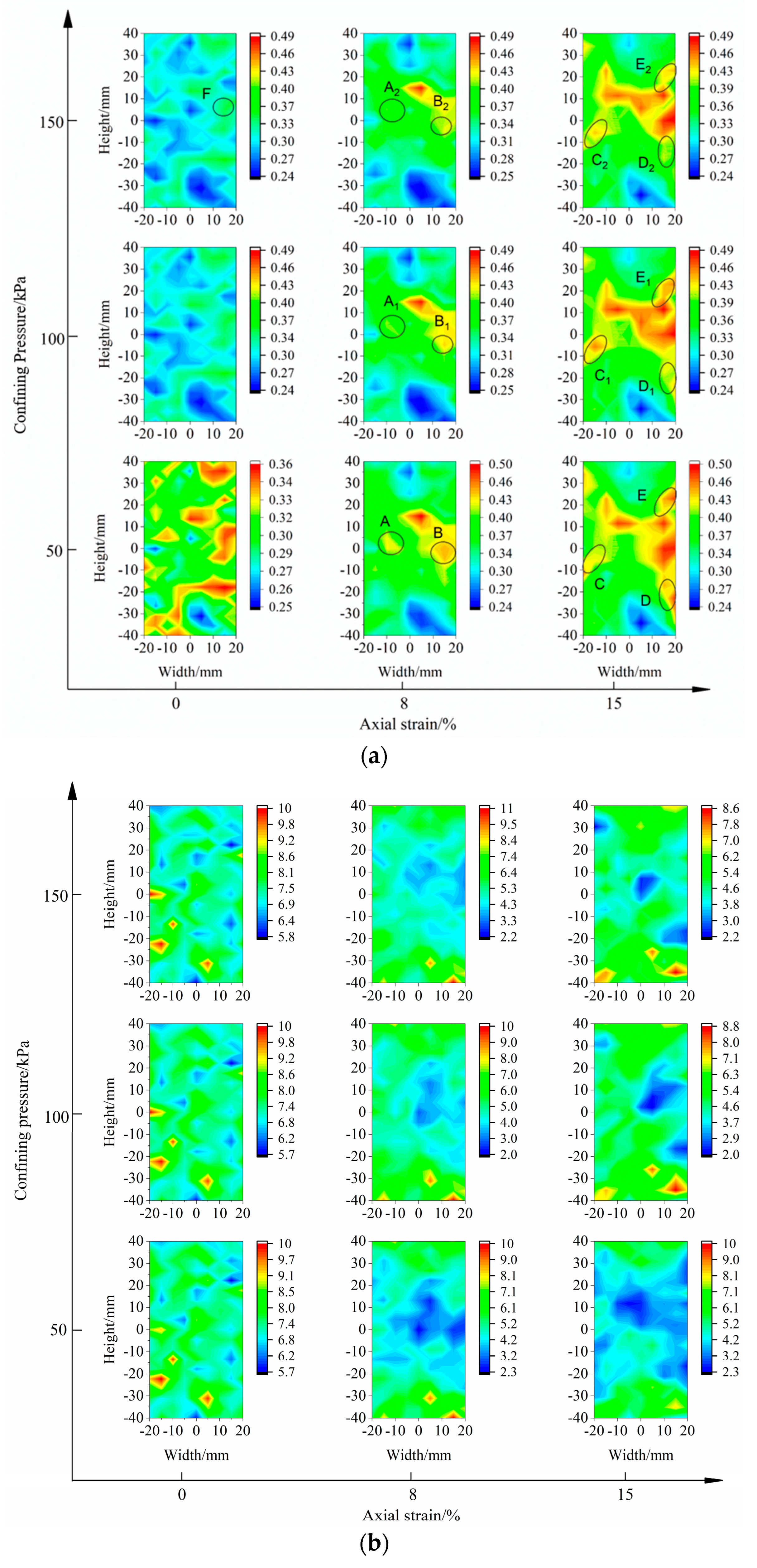
Figure 7 illustrates the arrangement of measurement spheres, and the corresponding porosity-versus-coordination-number cloud is presented in Figure 11. An analysis of Figure 11 reveals that as axial strain increases, both porosity and coordination number undergo continuous changes, and the shear zone originates from the lower right, extending toward the upper left.

In contrast to the existing literature, where Zhu et al. [44] documented cross-shear damage in dense sand samples, our study reveals distinct features. The shear band identified in our simulations shows an inclined orientation, and the initial heterogeneity of the specimen can explain this phenomenon.

Figure 11a provides a clear illustration: the porosity in the F region peaks at 0.35, representing the highest porosity at 0% strain. As axial strain increases, the shear band originates from this position and extends to form a through-shear zone. This observation highlights a crucial finding: the development of the shear band is closely linked to the initial state of the specimen.

As the axial strains reach 8% and 15%, the porosity in the A–E region steadily decreases with increased confining pressure (Figure 12). This decrease in porosity contributes to a narrowing trend in the width of the shear zone. Similarly, Figure 11b demonstrates that the region with a low coordination number progressively narrows and diminishes with the increase in confining pressure (Figure 12). This observation supports the idea of a gradually narrowing shear zone with increasing confining pressure.

This phenomenon can be attributed to the increased compactness of the specimen as the confining pressure rises. Lin demonstrated a clear correlation between material density and shear zone width, indicating that higher material density results in narrower shear zones [45]. Specifically, at 150 kPa, the average porosity decreases by 6% compared to that at 50 kPa. As a result, the particles become more tightly packed, restricting the formation of shear zones to a narrower region.

3.2.3. Stress–Strain Curves inside and outside the Shear Zone

To obtain stress–strain curves on both sides of the shear zone, three measuring balls were selected on the inner and outer sides of the shear zone, as depicted in Figure 7. The monitoring results are shown in Figure 13. In Figure 13, 1, 2, and 3 are obtained by monitoring measurement points 1, 2, and 3 within the shear zone, and 4, 5, and 6 are obtained by monitoring measurement points 4, 5, and 6 outside the shear zone.

Upon observation of Figure 13, it becomes apparent that the stress–strain relationship within and outside the shear zone exhibits distinct patterns. Specifically, the interior of the shear zone demonstrates a noticeable strain softening phenomenon, while the exterior displays unloading behavior. This phenomenon has been illustrated through finite element analysis, as described in reference [13].

This phenomenon can be attributed to the shear zone in which soil particles experience damage due to relative misalignment. As loading continues, the stress required to induce unit strain within the shear zone decreases, resulting in strain softening within the shear zone region. On the other hand, the region outside the shear zone experiences an increased stress requirement for failure due to the compression density effect. Therefore, as the soil within the shear zone experiences strain localization and softening, the soil outside the shear zone has not yet reached the critical stress needed for failure. This discrepancy results in the stress–strain curve unloading along a specific path.

4. Discussion

The primary objectives of this study are to conduct a comparative analysis between the utilization of flexible membranes and rigid walls, examine the influence of various boundary conditions on our simulation outcomes, investigate the particle size composition of a flexible membrane, and analyze the impact of particle size on our simulation results. The overarching goal of this research is to comprehensively understand the effects of these conditions on the behavior of granular materials.

In conclusion, this study offers compelling evidence to support the superior use of flexible membranes in accurately representing granular materials’ macroscopic behavior and deformation characteristics [25,26,27]. The flexible membrane device successfully simulated the experimental boundary conditions and effectively reflected the shear failure process of the specimens [28]. In contrast, the rigid wall setting was unable to capture essential phenomena, such as the generation of compression zones and the development of shear bands. This disparity can be attributed to the limitations of the rigid wall setting, which only allows for overall lateral deformation without considering protrusion deformation.

The flexible film, composed of pebble composite particles, faithfully replicated the behavior of actual samples by exhibiting protrusion deformation. Additionally, the flexible membrane setting allowed for the relative movement of particles within the sample, making it more representative of the conditions encountered in indoor model tests. This comprehensive representation led to a more accurate prediction of the macroscopic stress–strain behavior and deformation characteristics of granular materials.

Furthermore, this study provided novel insights into the development of shear bands. The observation revealed that shear bands initiate from the position with the highest porosity in the initially generated sample, suggesting that they originate from the weakest area. This finding contrasts with previous research and contributes a deeper understanding of shear band formation mechanisms.

Another distinctive aspect of this study involves the consideration of particle size within the flexible membrane device. Unlike previous studies that primarily focused on reducing boundary effects [28], our research highlights the significant influence of particle size on both the application of confining pressure and simulation accuracy. Our results demonstrate the influence of confining pressure and radius ratio on the simulation outcomes by exploring seven schemes involving different particle radii ranging from 2.5 mm to 0.25 mm. Maintaining a radius ratio within the range of 0.2 to 0.8 is crucial to balancing accuracy and efficiency. Ratios exceeding 0.8 result in increased roughness in the flexible film, leading to substantial deviations from the actual results. Conversely, ratios below 0.2 introduce excessive particles in the flexible film, increasing computational time and cost.

This investigation also provides insights into the stress–strain relationships inside and outside the shear band. Distinct behaviors were observed, with the external area of the shear band exhibiting unloading, while the internal area displayed strain softening. This phenomenon arises from the relative dislodgment and damage of soil particles within the shear band. As loading progresses, the stress required to induce unit strain in the shear band area decreases, resulting in strain softening. In contrast, the soil outside the shear band has not yet reached failure stress due to compaction effects, leading to unloading along a separate path on the stress–strain curve.

Surprisingly, this research reveals that increased confining pressure results in more concentrated strain localization and narrowing of the shear band. This can be attributed to the heightened compactness of the sample as the confining pressure escalates. Monitoring porosity demonstrates a 6% decrease in average porosity under 150 kPa confining pressure compared to 50 kPa confining pressure. The closely interlocked particles lead to shear bands occurring only in locally narrow areas.

In summary, this study effectively highlights the benefits of employing flexible membranes for simulating granular materials, leading to a more precise depiction of macroscopic behavior and deformation characteristics. This approach successfully captures the development of shear bands, surpassing the limitations of rigid wall devices. By monitoring porosity and considering particle size, this research substantially enhances our comprehension of shear band formation and the impact of boundary conditions. Choosing an appropriate radius ratio in the flexible membrane device achieves a balance between accuracy and efficiency in simulating stress–strain behavior. These findings make valuable contributions to advancing the understanding and prediction of the mechanical response of granular materials. They empower engineers to make well-informed decisions during the design and construction stages of infrastructure projects, ultimately enhancing the dependability and longevity of engineered structures.

5. Conclusions

This study utilized a numerical simulation method to examine the triaxial compression of a flexible membrane, with specific enhancements in applying confining pressure to the membrane. The investigation centered on the impact of flexible membrane particle size and conducted a comprehensive analysis of shear damage behavior in sandy soil from a fine-scale perspective, thereby surpassing the limitations of conventional macroscopic experiments. The simulation results produced noteworthy findings, offering valuable insights for soil engineering practice and setting the stage for future research endeavors.

Applying a flexible membrane in triaxial compression tests significantly improved the prediction accuracy of fundamental granular material properties, including the proportional limit and peak stress points. Significant improvements of 9.4% and 5.3% were achieved, along with successfully replicating shear expansion behavior. These outcomes provide reliable predictions for engineering applications, supporting structural design optimization and the development of effective soil engineering solutions.

This study emphasized the critical role of flexible membrane particle size within the range of 0.2 to 0.8 r. This carefully selected size range ensured excellent agreement between the simulation and experimental results, maintaining data stability. It offers a reliable guideline for future test designs, ensuring overall reliability and serving as a foundation for comprehensively exploring shear damage behavior in sandy soils.

A significant correlation was observed between the specimens’ initial state and the shear zone formation location. Specifically, shear bands tended to form in regions with larger initial porosity under certain initial conditions. This finding emphasizes the importance of considering initial states in engineering projects, especially in the context of soil engineering practice.

As the confining pressure increased, strain localization became more concentrated, leading to narrower shear zones. This observation reveals the evolving patterns of soil damage characteristics under varying confining pressure conditions.

An intriguing discovery was the distinct stress–strain relationships within the soil body on either side of the shear zone. The outer region displayed unloading behavior, while the inner part exhibited strain softening. This insight holds significance for understanding soil damage mechanisms and local behavior.

Strain localization, a geological phenomenon significantly affecting rock deformation and land stability, has considerable socio-economic implications that extend throughout communities and infrastructure. Targeted research focusing on shear zones offers a crucial pathway to sustainable development while reducing ensuing socio-economic disruptions. Integrating this research into land use planning and engineering design enables societies to minimize vulnerability to landslides and related hazards. This holistic approach safeguards human lives and notably alleviates enduring financial burdens on the local economy. The exploration of shear zones significantly influences infrastructure resilience and hazard mitigation, rendering it a fundamental tool for advancing sustainable geotechnical engineering practices and ensuring global socio-economic well-being.

However, it is essential to acknowledge the limitations of this study. The investigation did not consider soil body anisotropy, which affects the scope of the results. Furthermore, due to spatial and testing apparatus limitations, the focus was solely on one specimen size, disregarding the potential impact of specimen size on the outcomes. These limitations suggest promising directions for future research, aiming to enhance our understanding of shear damage behavior in sandy soils. Future studies should consider soil anisotropy in various engineering scenarios and explore the effects of different specimen sizes to develop a comprehensive understanding of the impact of these factors on study outcomes.