Application of a Semi-Empirical Approach to Map Maximum Urban Heat Island Intensity in Singapore

Abstract

Differences in land surface characteristics across a city produce great spatial and temporal variability in air temperature. This fact is particularly pronounced between urban and surrounding rural areas giving rise to the canopy-layer urban heat island (CL-UHI) phenomenon. In the present study, we apply the dimensional analysis technique to develop a simple semi-empirical equation to map daily maximum CL-UHI (UHI_max) intensities during nighttime over the city of Singapore for specific weather conditions. By adopting the methodology proposed by Theeuwes et al., but selecting meteorological and morphological parameters that affect UHI_max intensity most for Singapore, evaluation of the developed equation shows good agreement with observations (RMSE = 1.13 K and IOA = 0.76). Model performance depends strongly on wind conditions and is best during weak winds when ‘ideal’ conditions for UHI development are approached (RMSE = 0.65 K and IOA = 0.85). Results using the simple equation developed to map UHI_max intensities in Singapore under dry weather conditions are comparable to those obtained from more sophisticated numerical models, which demand significant computational resources, and the complex parameterizations involved require expertise to carry out the simulations. The resulting maps of the present study can be used to investigate less favorable thermal conditions and assess population vulnerability to a certain temperature excess, as well as provide insights for urban planning strategies of mitigation measures according to the land cover and morphology of a location.

1. Introduction

The urban heat island is a well-known phenomenon that has been studied since the early 19th century [1]. Of the various heat island types, the canopy-layer urban heat island (CL-UHI) is the most important one with regard to healthy and sustainable cities. It is quantified as the difference in near-surface air temperature between built-up areas and rural surroundings [2]. Numerous studies have focused on understanding and explaining the processes involved in this phenomenon in diverse urban environments around the world [3,4,5]. Urban morphology, land cover, and anthropogenic heat fluxes are key factors altering the local surface energy balance, which, together with geographical location and meteorological conditions, produce nocturnal heat islands of various intensities. In particular, the prevalence of impervious as opposed to natural surfaces in the city, the presence of buildings, and the high thermal admittance of urban materials increase the absorption of incoming shortwave radiation and storage of heat energy. Moreover, the available energy is preferentially partitioned into sensible at the expense of latent heat flux. All these factors contribute to a reduced nocturnal cooling rate in the city, which gives rise to higher urban–rural air temperature differences [6]. CL-UHI magnitudes are generally negatively (positively) correlated with the sky-view factor (street aspect ratio) [7,8,9], inverse relationships are found with the amount of urban vegetation [10,11,12], and local circulations such as the sea breeze have been shown to reduce urban heat [13,14].

The CL-UHI effect has been thoroughly studied using observations [15,16,17] and numerical models [18,19]. Monitoring studies can be expensive and time-consuming and are often limited to a few individual sites and meteorological conditions and are therefore not necessarily representative of air temperature variability across entire cities, weather conditions, or particular seasons. Numerical models instead are capable of estimating spatiotemporal patterns of CL-UHI intensity through sophisticated simulations but are approximations of reality and need to be properly validated. Numerous studies have focused on simulating the spatial variability of CL-UHI intensities in many different cities [19,20,21,22,23]. Some have also assessed model sensitivity to distinct urban parameterization schemes (e.g., single or multi-layer urban canopy models) [24,25]. However, all these models demand significant computational resources, and the complex parameterizations involved require expertise to carry out the simulations. Hence, more simple approaches, such as empirical models based on observations, have been developed to estimate spatial air temperature patterns and CL-UHI intensities. The relative simplicity of this empirical approach makes it easy to use; however, the application of such a model is restricted to conditions similar to those under which it was developed, e.g., for a particular location and specific weather conditions. The most common statistical approach uses multiple linear regression relationships between the CL-UHI and parameters known to influence its intensity [26,27,28,29]. However, these models do not provide much insight into the physical workings of the phenomenon. Alternatively, some studies use physically based equations and dimensional analysis based on Buckingham’s $\Pi$-theorem [30] to estimate CL-UHI patterns. This technique consists of extracting dimensionless variables based on the physical dimensions (e.g., time, mass) of physical quantities giving rise to a physically meaningful equation between independent variables. Previous studies using scaling methods have derived physically based equations to calculate CL-UHI intensities based on variables such as boundary layer height or surface sensible heat flux, which might not commonly be measured in other cities [31,32].

A more recent study by Theeuwes et al. [33] (hereafter referred to as T17) developed a diagnostic equation to calculate the nocturnal maximum CL-UHI intensity using commonly measured standard weather variables such as air temperature, radiation, and wind speed. Empirical models are usually designed for a single study city; however, T17 proved that this equation was giving good results in the 14 European cities studied. To our knowledge, at least two studies have applied the equation developed by T17 in Chinese cities. Results from the humid subtropical city of Xi’an [34] and the temperate climate city of Nanjing [35,36] show reasonable agreement with observations, although model–observation correlations were slightly worse than those obtained by T17. Hence, Zhang et al. [34] adapted the original equation to the target city in order to better represent the local characteristics.

The main objective of the present study is to develop a simple semi-empirical equation using basic climate and urban land cover parameters to estimate daily maximum CL-UHI intensity (UHI_max) using long-term observations in tropical Singapore. To achieve this purpose, we adapt the methodology proposed in T17 to better represent the local characteristics of Singapore. A number of past studies have already analyzed the spatial and temporal evolution of CL-UHI intensity over Singapore using observations [37,38,39] and numerical simulations [40]. However, the present study provides an alternative method to estimate spatial patterns of maximum CL-UHI intensities that is easy to apply and provides detailed spatial information on the local-scale air temperature variability under selected meteorological conditions. Section 2 provides a description of the study area, observation network, local climate, and urban morphological characteristics of Singapore. The original T17 model is applied to Singapore in Section 3. Section 4 introduces the modified model for Singapore, which is evaluated in Section 5. Maps of UHI_max intensities for different weather conditions are shown in Section 6, followed by a discussion and concluding remarks in Section 7.

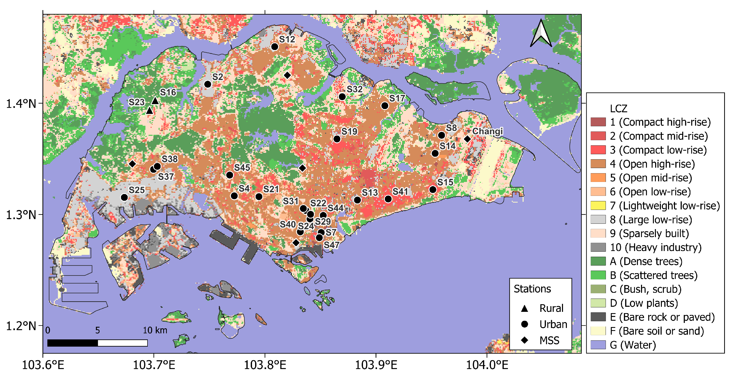
2. Study Area, Observational Data, and Urban Morphological Characteristics

Singapore is an island city-state located close to the equator (1°21′ N, 103°49′ E) occupying an area of ∼722.5 km² [41] (Figure 1). Most of the terrain is low-lying with little change in topography across the island. The highest point is 168 m a.s.l., located in a nature reserve close to the center of the island, which is also home to several freshwater reservoirs. Regarding land cover classification, the local climate zone (LCZ) scheme is sometimes used to divide the landscape into regions of uniform surface cover, structure, material, and human activity, having a characteristic CL air temperature [42]. The LCZ map for Singapore is developed using Google Earth Engine, a cloud-based platform for planetary-scale geospatial analysis [43,44]. The procedure consists of classifying several times the training areas developed for Singapore into LCZ categories, using satellite data products within the period 2014–2016, and the final LCZ map comprises the modal category [45]. The most predominant built type region in Singapore is LCZ 4 (open high-rise), followed by LCZs 9 (sparsely built) and 8 (large low-rise), respectively (Figure 1, [45]).

Observations obtained between August 2011 and May 2014 are used in the present study with experimental details fully explained in Roth et al. [39] (referred to as R22 hereafter). Briefly, a network of sensors installed specifically to measure air temperature at a height of 2–3 m above ground provides locally representative observations. Twenty-four sensors are located in urban areas and two in rural areas representing the rural ‘reference’ (Figure 1). Sensor locations were chosen to represent maximum thermal differences between neighborhoods representing a wide range of LCZ classes found in Singapore. Relevant key features of the 26 stations used are summarized in

Table 1. Coordinates, morphological and land cover characteristics of measurement stations. SVF—sky-view factor, H/W—height-to-width ratio, $F_{urb}$—urban fraction, $F_{veg}$—vegetation fraction, LCZ—local climate zone. LCZ 1 (compact high-rise), LCZ 2 (compact midrise), LCZ 3 (compact low-rise), LCZ 4 (open high-rise), LCZ 5 (open midrise), LCZ 6 (open low-rise), LCZ 8 (large low-rise), LCZ A (dense trees), and LCZ B (scattered trees) [42].

Station ID	Lon (°)	Lat (°)	Local SVF	$\mathit{H}/\mathit{W}$ (300-m Average)	${\mathit{F}}_{\mathit{urb}}$ (300-m Average)	${\mathit{F}}_{\mathit{veg}}$ (300-m Average)	LCZ
Urban stations
S2	1.4171	103.7485	0.69	0.41	0.88	0.10	8
S4	1.3167	103.7724	0.19	0.20	0.44	0.47	A/4
S7	1.2837	103.8507	0.19	5.16	0.87	0.06	1
S8	1.3712	103.9591	0.37	0.97	0.64	0.31	4
S12	1.4509	103.8088	0.55	0.44	0.85	0.10	8
S13	1.3129	103.8833	0.66	0.96	0.84	0.13	2
S14	1.3549	103.9533	0.32	0.94	0.76	0.19	4
S15	1.3223	103.9512	0.67	0.76	0.75	0.20	3
S17	1.3978	103.9080	0.47	1.83	0.77	0.20	4
S19	1.3679	103.8649	0.84	0.77	0.76	0.19	3
S21	1.3160	103.7946	0.54	0.61	0.43	0.56	6
S22	1.3035	103.8369	0.24	2.49	0.82	0.17	1
S24	1.2960	103.8406	0.55	1.52	0.68	0.30	5
S25	1.3153	103.6734	0.56	0.39	0.90	0.07	8
S29	1.3001	103.8411	0.52	1.18	0.69	0.30	4
S31	1.3053	103.8346	0.70	2.15	0.82	0.17	3
S32	1.4059	103.8696	0.78	0.14	0.30	0.70	6
S37	1.3405	103.6997	0.70	0.99	0.70	0.25	4
S38	1.3432	103.7031	0.26	1.52	0.69	0.28	4
S40	1.2844	103.8319	0.44	0.63	0.70	0.28	5
S41	1.3139	103.9110	0.86	0.88	0.78	0.18	3
S44	1.2991	103.8525	0.41	1.84	0.91	0.09	1/2
S45	1.3354	103.7683	0.79	0.74	0.76	0.24	3
S47	1.2791	103.8490	0.14	3.81	0.91	0.09	1
Rural stations1
S16	1.4028	103.7012	0.66	0.01	0.08	0.9	B
S23	1.3939	103.6961	0.83	0.01	0.07	0.9	B

¹ Air temperatures from S16 and S23 are averaged to calculate the rural reference air temperature.

, which lists station coordinates and the morphological and land cover characteristics within a 300 m grid covering the respective station. Except for the local sky-view factor (SVF), which is obtained at the actual station location, urban parameters represent average values across a 300 m × 300 m grid cell closest to the station used in a recent numerical modeling study [46]. Also, 300 m × 300 m corresponds to the footprint or source areas of canopy-layer air temperature sensors (see, e.g., [39]). Data from an additional five weather stations operated by the Meteorological Service of Singapore (MSS) are employed to select days without rainfall (Figure 1). Finally, synoptic weather conditions are characterized using solar radiation, 2 m air and dew-point temperatures, and 10 m wind speed collected at the MSS Changi weather station (Figure 1).

Daily UHI_max magnitude is computed as the maximum difference of hourly air temperature at any urban station ($T_{2m,urb}$) minus the air temperature at the rural reference station ($T_{2m,rur}$) during nighttime (from 20 LT to 06 LT): UHI_max = $T_{2m,urb}-T_{2m,rur}$. Here, $T_{2m,rur}$ is calculated as the average of stations S16 and S23 (see R22 for further explanations on the selection of the rural reference sites). R22 presents a detailed analysis of the effect of weather on CL-UHI, with the highest magnitudes observed during dry, calm, and clear nights. Using the same filtering approach for ‘ideal’ conditions as in R22 leaves only 36 nights or 3.5% of the entire dataset. This sample size is too small for rigorous analysis. Hence, the present study only filters for rainfall by excluding days with >0.2 mm rainfall measured simultaneously at the five MSS stations. The remaining dataset for further analysis comprises 303 dry days (30% of the original data).

3. Application of Diagnostic Equation Proposed in Theeuwes et al. [33]

Below we apply the diagnostic equation proposed by T17 and evaluate its performance in the context of tropical Singapore. T17 derives the following relationship based on dimensional analysis and using routine weather observations and standard land cover and morphological parameters:

$$\begin{array}{c}\hfill {\mathrm{UHI}}_{\max }=(2-SVF-F_{veg})\sqrt[4]{\frac{K_{in}·DT{R}^3}{U_{24h,av}}}\end{array}$$

(1)

Here, $K_{in}$ is the downward shortwave radiation in kinematic units (K m s⁻¹)), DTR the daily temperature range (DTR (K) = $T_{max}-T_{min}$), and $U_{24h,av}$ the 24 h average 10 m wind speed (m s⁻¹), all measured at a rural reference site. The SVF at the station location is estimated from building height and street width data, and $F_{veg}$ is the vegetation fraction within a 500 m circle centered on the urban station. Equation (1) is only valid over the parameter range for which it has been developed, which for SVF and $F_{veg}$ are 0.2 to 0.9 and 0 to 0.4, respectively. Hence, our stations S4, S7, S21, S32, and S47 are excluded from the evaluation. Also, since the present study did not measure $K_{in}$ and $U_{24h,av}$ at our rural sites, we use respective data from the Changi weather station (Figure 1). Given that Changi is an official WMO weather station (WMO Index Number: 48698) and considering the absence of significant topography and little variability of synoptic conditions across the relatively small size of Singapore, we assume that the Changi data is representative of regional weather and hence similar day-to-day variability is expected to that at the rural sites. Therefore, using $K_{in}$ and $U_{24h,av}$ at Changi station, DTR measured at the rural site and SVF, and $F_{veg}$ from Table 1, the proposed equation in T17 (Equation (1)) is applied to predict UHI_max intensities at 19 urban stations for the 303 dry days of the study period. Modeled UHI_max magnitudes are compared with observed UHI_max intensities at the selected urban stations (Figure 2a).

Model accuracy is quantified using the index of agreement (IOA) and Pearson correlation coefficient (R), and the root mean squared error (RMSE) and median absolute error (MEAE) are used to calculate model deviations from observations. Although the errors appear acceptable (RMSE = 1.10 K and MEAE = 0.75 K), UHI_max is slightly overestimated, and the relationships show considerable scatter (Figure 2a).

Compared to previous studies using the same approach, model error statistics are similar to those obtained for European cities (RMSE = 0.91 K and MEAE = 0.58 K) (T17) or Nanjing (RMSE = 1.00 K and MEAE = 0.68 K) [36]. However, the present R value is significantly lower, 0.37, compared to 0.81 and 0.67, respectively. The poor performance of the model for Singapore is hypothesized to be due to a combination of reasons:

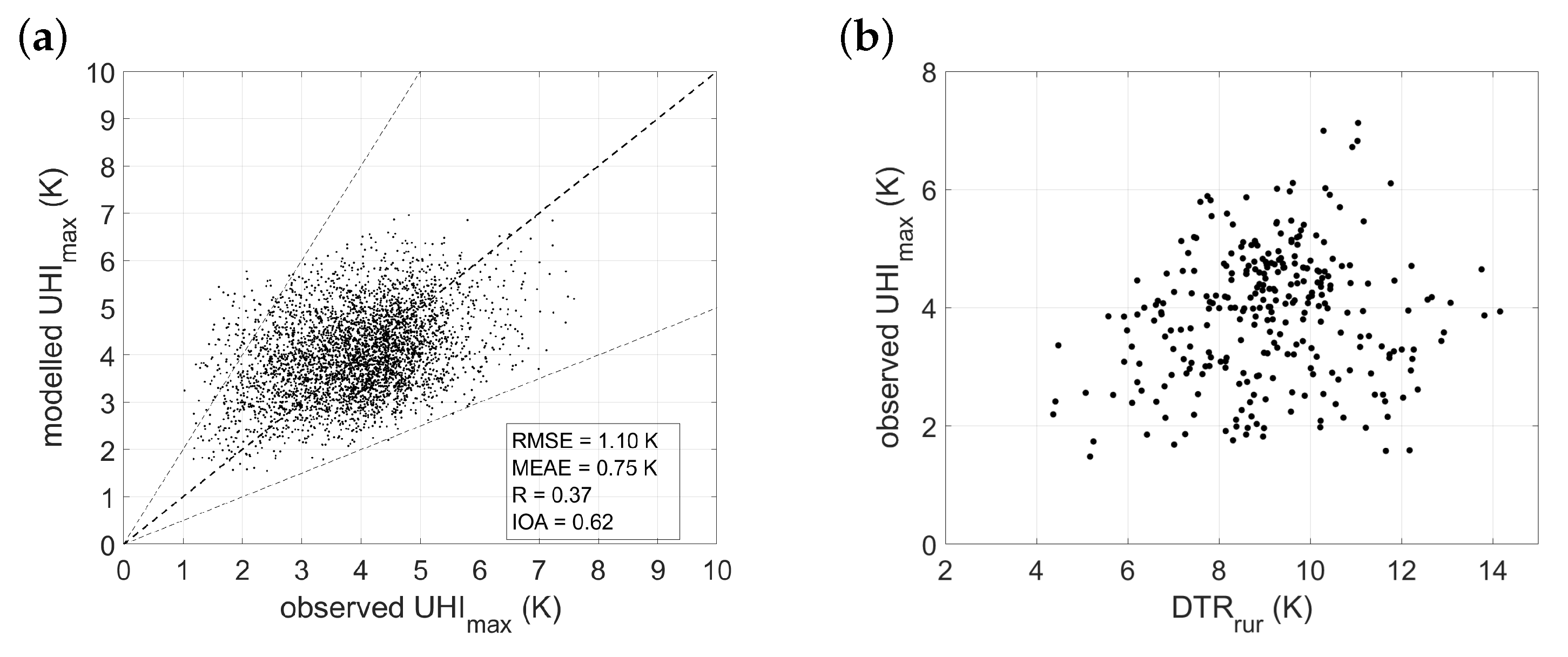
• Different reference stations are used for the weather variables. $K_{in}$ and $U_{24h,av}$ are mainly considered in the equation to determine the seasonal variability of weather conditions within the study period. Although similar day-to-day variability is expected at Changi compared to the rural site, the magnitude, particularly for wind speed, might vary.
• The rural reference sites are characterized by different land cover types. LCZ D (low plants) is used in T17, but LCZ B (scattered trees) in the present study. DTR for the former is therefore likely larger since daytime air temperature will be higher over an open area, compared to a partially shaded area. This discrepancy could be responsible for the large scatter in Figure 2b, as compared to the strong relationship between UHI_max and DTR observed in T17.

Although model errors are comparable to those obtained in other cities, empirical equations are restricted to circumstances similar to those under which they were derived. The established ranges for urban parameters (SVF and $F_{veg}$) also exclude some stations representative of specific areas of Singapore (e.g., S7 (LCZ 1) in the business district). Given the important differences in the local climate context, we therefore develop in the next section a similar equation following the same methodology proposed by T17, but selecting meteorological and morphological parameters that provide better explanatory power for UHI_max intensities for the specific local climate and urban geometry of Singapore.

4. Development of the Model Equation for Singapore

The empirical equation developed here is based on relationships between independent variables thought to significantly affect UHI_max intensities. A set of dimensionless groups is defined from such variables through dimensionless analysis [30], from which a relationship with UHI_max is determined empirically using data from 24 urban stations and 303 dry days.

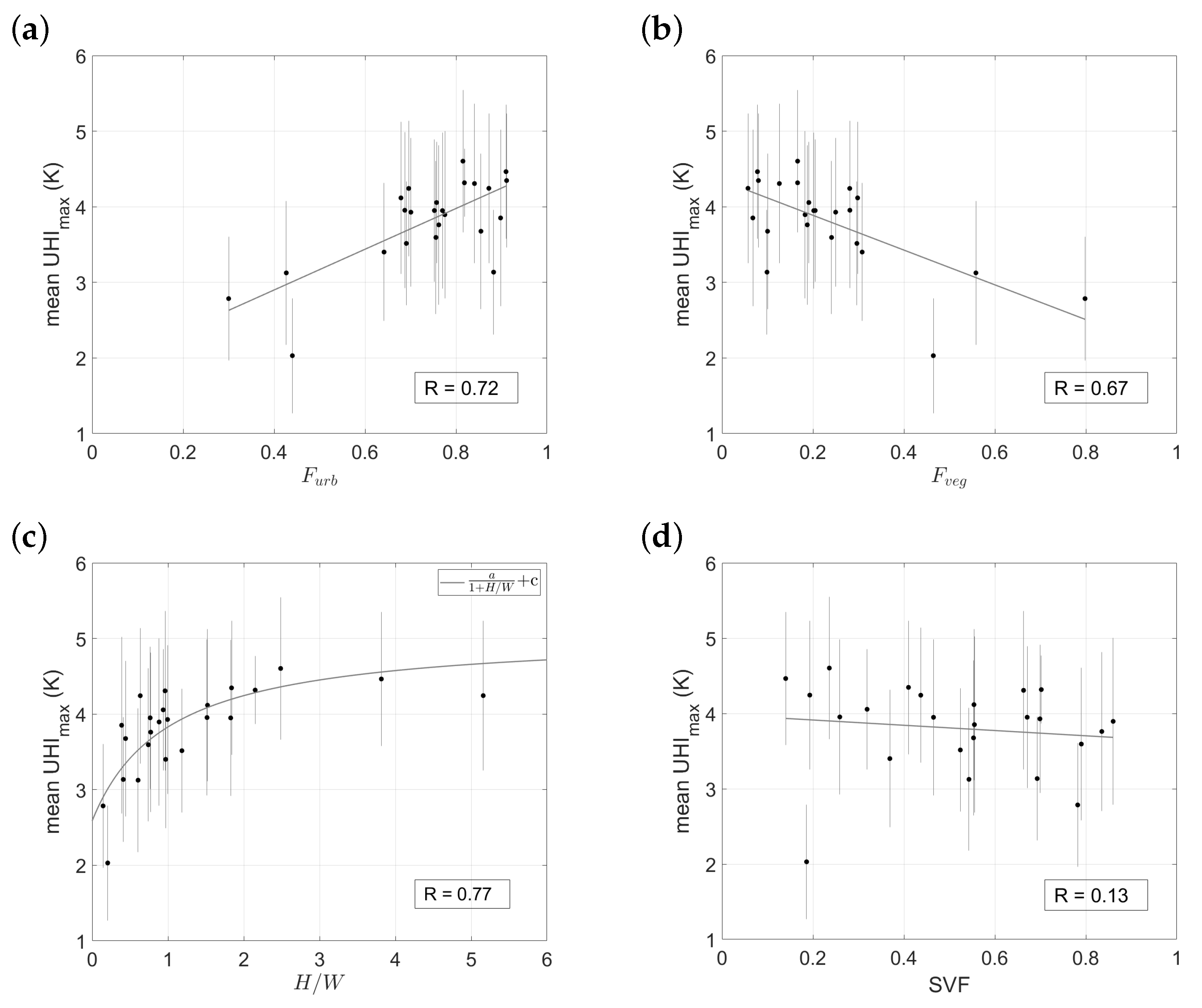
4.1. Selection of Independent Variables

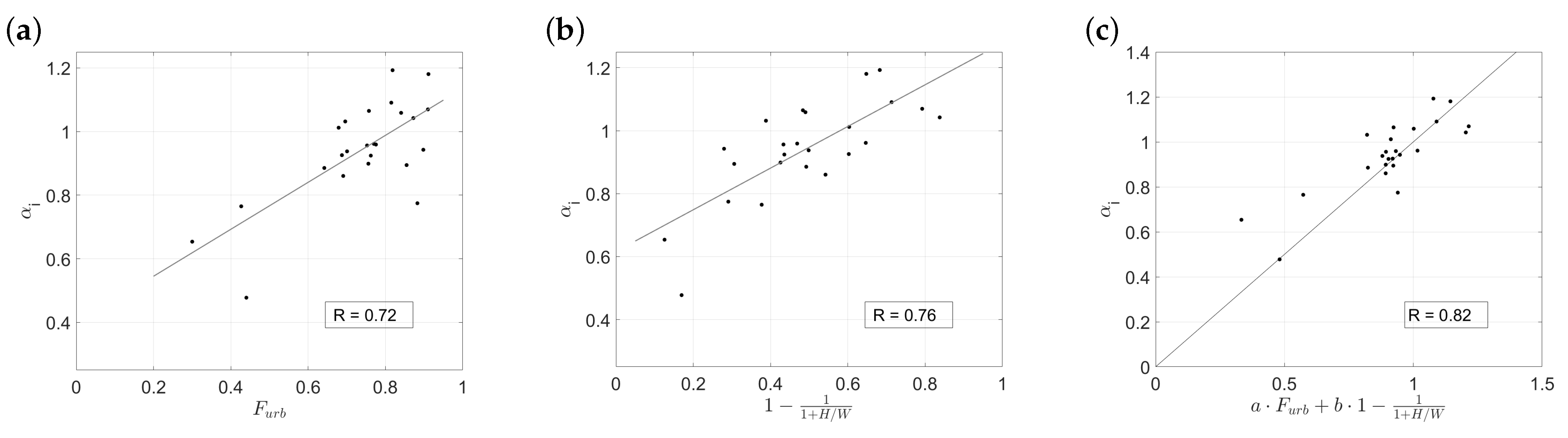
4.1.1. Land Cover and Morphological Parameters

Land cover and morphological parameters are key factors in generating nighttime intra-urban differences in air temperature and hence CL-UHI magnitude [2]. As expected, UHI_max increases with urban fraction ($F_{urb}$) and decreases with $F_{veg}$, with a slightly lower correlation coefficient for the latter (Figure 3). Street geometry can be characterized by street aspect ratio (H/W) and SVF. In the present study, H/W is the average for an area within a 300 m circle centered on the station, and SVF is determined from fisheye images at the actual station location [47]. Scatter plots do not reveal a clear trend of UHI_max with the local SVF (R = 0.13, Figure 3d). On the other hand, a good fit in the form of an exponential relationship is found for H/W (R = 0.77, Figure 3c). Therefore, $F_{urb}$ and H/W are selected as key independent variables to build our model.

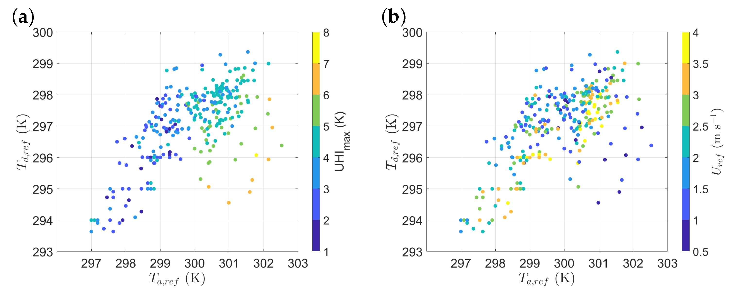
4.1.2. Meteorological Variables

Meteorological conditions influence UHI development and are therefore important to determine urban–rural differences [2,39]. Here, we select representative meteorological variables that are known to affect daily and seasonal UHI_max intensity.

Wind limits the development of the CL-UHI, the latter being largest under calm conditions [39,48]. Wind speed measured at 10 m a.g.l. ($U_{ref}$) is chosen as one of the key variables in the model. In addition, clear skies promote strong daytime insolation and larger nighttime UHI intensity given that surface cooling driven by longwave radiation loss is slower in urban than rural environments. Incoming shortwave radiation ($K_{in}$) reflects the day-to-day variability of the energy that reaches the urban surface and hence can be used as a proxy of daytime cloud conditions, with the assumption that similar conditions extend into nighttime.

Soil moisture also contributes to CL-UHI development and variability (e.g., [49]). Wet rural soils will have a higher heat capacity (and thermal admittance) and hence slow nighttime cooling, which will result in a reduced UHI intensity. To some extent, this variable is already considered by selecting dry days only. However, soil moisture also varies within dry days depending on how much time has passed since a particular rainfall event. The proposed model also considers a reference air ($T_{a,ref}$) and dew-point ($T_{d,ref}$) temperature measured at Changi station. The ratio between $T_{a,ref}$ and $T_{d,ref}$ is an indirect measure of relative humidity and can be used to detect changes in atmospheric humidity due to short-term rainfall events as well as seasonal rainfall variability throughout the year. A positive trend is observed between UHI_max and $T_{a,ref}$ and $T_{d,ref}$ (Figure 4a), except for the highest magnitudes (UHI_max > 6 K). The reason for this is that UHI_max is at the time also affected by other meteorological variables and hence the difficulty to find an individual relationship with only one parameter. The scatter points with the highest UHI_max intensities in Figure 4a occur for high $T_{a,ref}$ but low $T_{d,ref}$, which would indicate air humidity diminishes, and it also coincides with low wind speed conditions ($U_{ref}$ < 1.5 m s⁻¹) (Figure 4b). We therefore use $T_{a,ref}$, $T_{d,ref}$, $U_{ref}$, and $K_{in}$ as indicators of further weather variability within the 303 dry days selected.

4.2. Development of the Model Equation for Singapore

To develop the equation, the dataset is randomly split into two subsets: 70% (212 nights) of the data are used to build the model and 30% (91 nights) to evaluate model performance. More data are employed to design the model to ensure the inclusion of greater variability of weather conditions. From above, the selected meteorological variables are $K_{in}$ in its kinematic form (K m s⁻¹), nocturnal $U_{ref}$ (m s⁻¹), $T_{a,ref}$ and $T_{d,ref}$ (K) measured at the reference Changi station, as well as land cover and morphological characteristics $F_{urb}$ and H/W, respectively.

Given that $F_{urb}$ and H/W are dimensionless, dimensional analysis is only applied to the meteorological variables, with the primary dimensions being temperature, length, and time. The application of Buckingham’s $\Pi$-theorem (Appendix A) results in two independent dimensionless groups,

$$\begin{array}{c}\hfill {\Pi }_1=\frac{{\mathrm{UHI}}_{\max }}{T_{a,ref}};{\Pi }_2=\frac{K_{\downarrow }}{T_{d,ref}·U_{ref}}\end{array}$$

(2)

The function relating ${\Pi }_1$ and ${\Pi }_2$ is derived from observations such that ${\Pi }_1=f\left({\Pi }_2\right)$. Considering that f might have a linear or exponential form, ${\Pi }_1=\alpha {\Pi }_2^{\beta }$. The latter is written as $log\left({\Pi }_1\right)=\beta ·log\left({\Pi }_2\right)+log\left(\alpha \right)$ to find the best linear fit for each station (Figure 5).

The linear fit for each station provides the best fit with a slope of $\beta$ = 0.6 (3/5) for all stations. Hence, the relationship between ${\Pi }_1$ and ${\Pi }_2$ can be written as ${\Pi }_1={\alpha }_i{\Pi }_2^{(3/5)}$, where subscript i refers to each individual station. Unlike $\beta$, parameter $\alpha$ varies from station to station as a function of land cover and morphological characteristics: $\alpha =f(F_{urb},H/W)$. The dependency on $H/W$ is reformulated as $1-\raisebox{1ex}{$1$}\!\left/ \!\raisebox{-1ex}{$\left(1+H/W\right)$}\right.$ to obtain a positive linear trend and avoid undefined results when H/W = 0. Scatter plots between $\alpha$ and the morphological characteristics, $F_{urb}$ and H/W, for all stations, show linear trends with reasonably high correlation coefficients of R = 0.72 and R = 0.76, respectively (Figure 6a,b). Hence, $\alpha$ can be estimated as $\alpha =a·F_{urb}+b·\left(1-\raisebox{1ex}{$1$}\!\left/ \!\raisebox{-1ex}{$(1+H/W)$}\right.\right)$, where coefficients a and b are determined using a simple regression model to arrive at $\alpha =0.9·F_{urb}+0.5·\left(1-\raisebox{1ex}{$1$}\!\left/ \!\raisebox{-1ex}{$(1+H/W)$}\right.\right)$ (Figure 6c).

Replacing the latter expression and rewriting the two dimensionless groups (${\Pi }_1$ and ${\Pi }_2$) as ${\Pi }_1={\alpha }_i{\Pi }_2^{3/5}$, the final equation to estimate UHI_max magnitudes over Singapore becomes:

$${\mathrm{UHI}}_{\max }=\left[0.9·F_{urb}+0.5·\left(1-\frac{1}{1+H/W}\right)\right]·{\left(\frac{T_{a,ref}^{5/3}·K_{in}}{T_{d,ref}·U_{ref}}\right)}^{3/5}$$

(3)

5. Model Evaluation

The performance of Equation (3) is evaluated with the observed UHI_max using the test dataset (Figure 7). Model results show an acceptable agreement with observations (IOA = 0.76) and R = 0.58 (Figure 7) and slightly improve compared to applying the model equation (Equation (1)) proposed by T17 (Figure 2). Overall, the model slightly underestimates observed UHI_max and error metrics are similar to those observed in other studies using Equation (1) (

Table 2. Model performance metrics to estimate UHI_max.

Dataset	IOA	RMSE (K)	MEAE (K)	R
Theeuwes et al. [33]—European cities		0.91	0.58	0.81
Zhang et al. [34]—Xi’an (China)		1.68	1.14	0.67
Yang et al. [36]—Nanjing (China)		1.00	0.68
Theeuwes et al. [33]—Singapore	0.62	1.10	0.75	0.37
Equation (3) for Singapore	0.76	1.13	0.79	0.58

).

Using the same dataset, we also analyze model performance at selected individual stations representing the range of urban LCZs present in the study area (Figure 8). Values of RMSE range between 0.9 and 1.3 K, being of the same order of magnitude as those obtained using physically based mesoscale models applied over the same study area [46,50]. The statistical model captures UHI_max variability across the selected stations with IOA varying between 0.59 and 0.76. The worst model agreement is obtained at S21 (LCZ 6). This is likely due to the low number of data points at the low end of $F_{urb}$, since only three urban stations have $F_{urb}$ below 0.45.

Figure 8 also shows the capability of the model to estimate the variability of UHI_max as a function of weather conditions variability. Further analysis at the individual station level reveals that scatter increases with stronger reference wind speed (not shown). Hence, further analysis is conducted to quantify model accuracy as a function of $U_{ref}$ (Figure 9). Absolute errors calculated as the difference between modeled and observed UHI_max magnitudes for all stations confirm that the smallest differences (<1 K) are usually found when $U_{ref}$ is <2.5 m s⁻¹ (Figure 9). Equation (3) is mainly developed to estimate UHI_max intensities according to urban parameters, whose influence on UHI development is most pronounced under calm wind conditions. The best performance of the model is therefore obtained for low reference wind speeds (

Table 3. Model performance metrics using the test dataset (91 nights) and entire period (303 nights) for two wind speed regimes.

Wind Speed Ranges	Test Period				Entire Period
	IOA	R	RMSE	MEAE	IOA	R	RMSE	MEAE
$U_{ref}$ < 2.5 m s−1	0.86	0.76	0.95	0.64	0.81	0.66	0.99	0.68
$U_{ref}$ > 2.5 m s−1	0.49	0.31	1.33	1.03	0.70	0.50	1.18	0.84

), which correspond to the largest UHI_max values and maximum influence from local characteristics (e.g., H/W and $F_{urb}$).

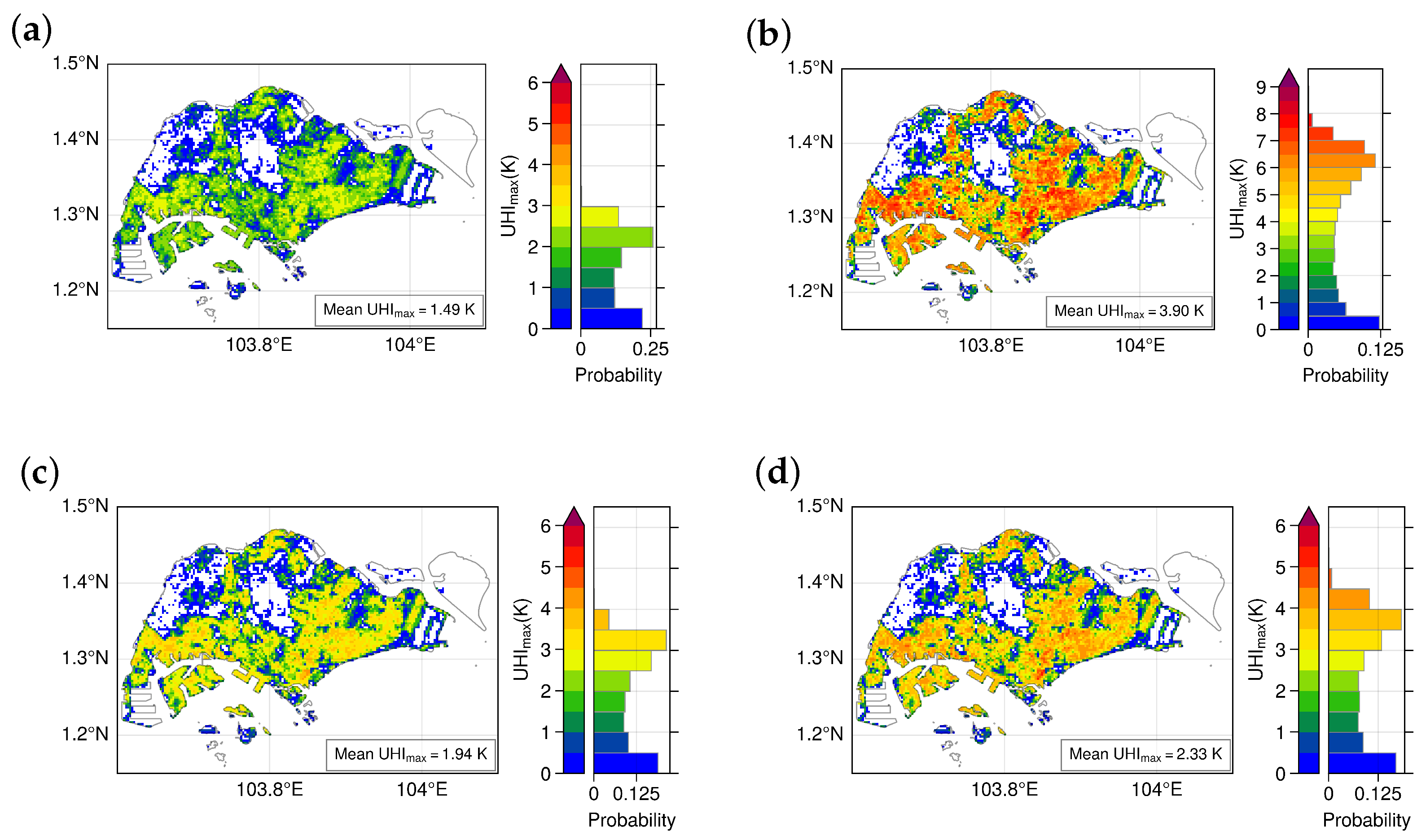
6. Mapping Spatial Patterns of UHI_max Intensities

Using morphological data available for the entire city at 300 m × 300 m resolution [46], the model can be applied to generate maps of UHI_max intensity under dry conditions for different seasons. Figure 10 shows the spatial distribution of UHI_max calculated as the mean of 36 ‘ideal’ (dry, calm, and clear) nights within the study period. The corresponding scatter plot reveals a very good correlation with observations (R = 0.85) and low prediction errors (RMSE = 0.65 K and MEAE = 0.55 K) (

Table 4. Model performance metrics for different periods and weather conditions.

Case	IOA	R	RMSE (K)	MEAE (K)
‘Ideal’ conditions	0.85	0.85	0.65	0.55
Lowest UHImax—5 February 2012	0.55	0.80	0.94	0.84
Largest UHImax—19 June 2013	0.89	0.86	0.90	0.52
mean UHImax for February	0.82	0.83	0.57	0.55
mean UHImax for June	0.72	0.83	1.01	0.90

). These evaluation metrics confirm the better performance of the model during low wind conditions, which coincides with the maximum UHI_max intensity (Figure 10b).

The largest UHI_max intensities reach 5.5–6.0 K covering around 1% of the total area and are mainly located in the densely built-up financial and business districts (LCZ 1) close to the south-central coast. Other areas with UHI_max > 4.5 K can be found in high-density residential districts (LCZ 2) in the southeast and industrial areas (LCZ 8) in the southwest of Singapore. The spatial average of the modeled UHI_max across built-up areas is 2.64 K, which can be interpreted as the maximum nighttime city-wide average air temperature increment caused by the presence of the city. The most frequent UHI_max intensity range across the city is between 4.0 and 4.5 K, covering 16.4% of the urban area. The second most frequent range of 0.0–0.5 K covers 15.4% of the built-up area and is found next to the coast or bordering reservoirs, parks, and secondary rainforests. In addition, the gridded model results for the mean UHI_max are used to analyze the spatial distribution based on the urban LCZ classification by resampling the original (100 m) map [45] to the present 300 m resolution (Figure 10c). The highest UHI_max intensities are found in LCZs 2 and 1, with the highest magnitude of 6.1 K corresponding to a grid cell pixel located in the business district belonging to LCZ 1. The distribution of the spatial analysis follows the expected variability of urban–rural differences as a function of the LCZ class [42]. The present results are similar to those observed in previous studies in Singapore under ‘ideal’ heat island conditions [37,39] and support the utility of the present simple statistical modeling approach.

Additional maps represent the typical seasonal variability in Singapore (Figure 11). They include monthly average maps based on dry days for the entire study period corresponding to the month with the generally lowest and highest UHI magnitudes in February and June, respectively [37,39]. Also shown are the maps for two individual nights with the lowest and highest daily UHI_max observed across all stations during the study period. UHI_max variability across the city is low on 5 February 2012, with the most frequent UHI_max magnitude band of 2.0–2.5 K covering 25.7% of the total built-up area (Figure 11a). Maximum values barely exceed 3.0 K (0.3% of the area), and the average nighttime temperature increment due to built-up areas across the city is 1.49 K. Comparison with observations shows good model performance (Table 4). February is part of the Northeast monsoon season and characterized by cloudy and rainy conditions, but the model nevertheless works well for dry periods during this otherwise wet month.

Spatial UHI_max variability is much larger when values are higher, as shown by the map for 19 June 2013 (Figure 11b). Five stations recorded their highest UHI_max intensity on this day, with the highest value of 7.53 K observed at S07 (LCZ 1) [39]. June coincides with the inter-monsoon period, which is characterized by calm winds and clear skies, both of which maximize heat island development and hence differences across different land covers. Unlike for February, the UHI_max probability distribution shows larger magnitudes and hence larger differences across different urban areas. The most prevalent UHI_max temperature bin is 6.0–6.5 K and covers 11.6% of the built-up area. Maximum intensities reach between 8.0 and 8.5 K. This is slightly higher than what was observed, but this particular range is only modeled over 0.1% of the built-up area, and 5% of the area shows UHI_max values > 7.0 K as observed at five stations. This confirms that the model is able to accurately capture the peak UHI_max values during these conditions. Model error metrics more generally also suggest good performance for this particular day (Table 4). The available spatial data also enable predicting the area (and population) exposed to a certain urban temperature excess, an important measure related to human thermal comfort. In the case of this particular day, 50% of the city’s built-up area, for example, was experiencing an UHI_max of 4.5 K or higher.

The corresponding monthly average maps confirm the generally lower (larger) UHI_max values and variability across the city experienced in February (June) (Figure 11c,d), as a result of the particular weather conditions in each month pointed out above. The spatial distribution is similar in both months, with the highest and lowest UHI_max values obtained over the more heavily built-up and greener areas, respectively. The maximum February (June) UHI_max values do not exceed 4.0 (5.0) K, and the probability distribution peaks between 3.0 and 3.5 (3.5–4.0) K, with ∼50% of the built-up area experiencing UHI_max values > 2.0 (2.5) K. Highest values always correspond to the south-central coast classified as LCZ 1. The mean UHI max across all built-up areas in February (June) is 1.94 (2.33) K. The model evaluated across all days of the respective month shows again good performance with a high R of 0.83 and prediction errors of between 0.52 and 1.01 K (Table 4).

7. Summary and Conclusions

A semi-empirical equation is derived to estimate daily UHI_max intensities in Singapore using the dimensional analysis technique and long-term (∼3 years) observations. The main purpose is to generate a simple and fast method to map the spatial distribution of UHI_max for dry weather conditions based on $F_{urb}$ and H/W.

We first tested the equation proposed by T17 for European cities for Singapore using the available weather data. The comparison of the model with observations results in slightly higher prediction errors but relatively low agreement compared to those obtained in T17. This discrepancy is hypothesized to be partly due to the present weather reference values ($K_{in}$ and $U_{ref}$) not being obtained at the rural reference site, but rather an official weather station. A more important reason for the differences is, however, the choice of the rural reference site which is grass and cropland in T17, but scattered trees in the present study. This will influence the cooling behavior of the rural environment and therefore alter the relationship between UHI_max and DTR [33]. We therefore develop a similar statistical model but adapted to predict UHI_max intensities during dry conditions in Singapore using the methodology proposed in T17. The main results are as follows:

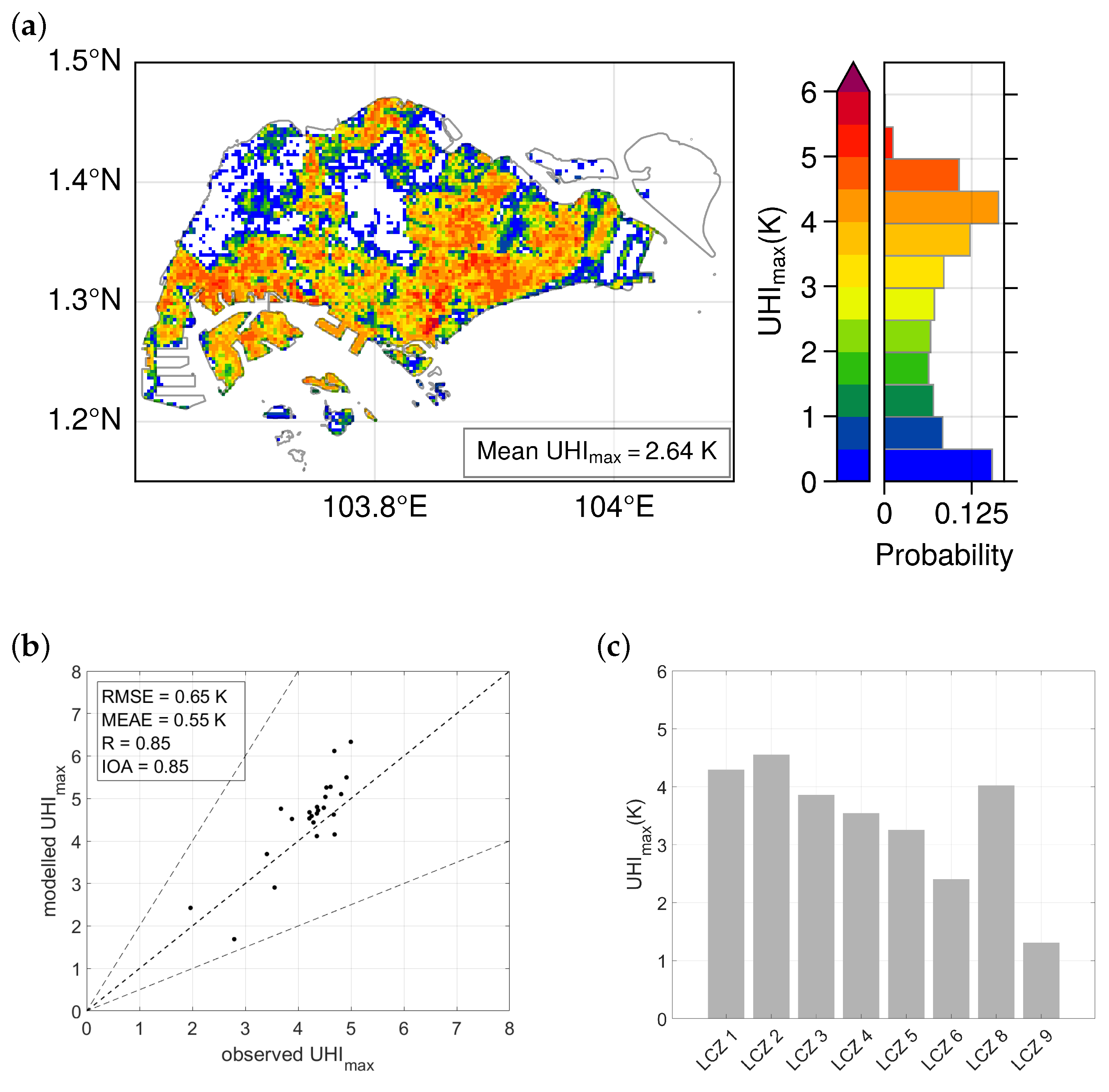
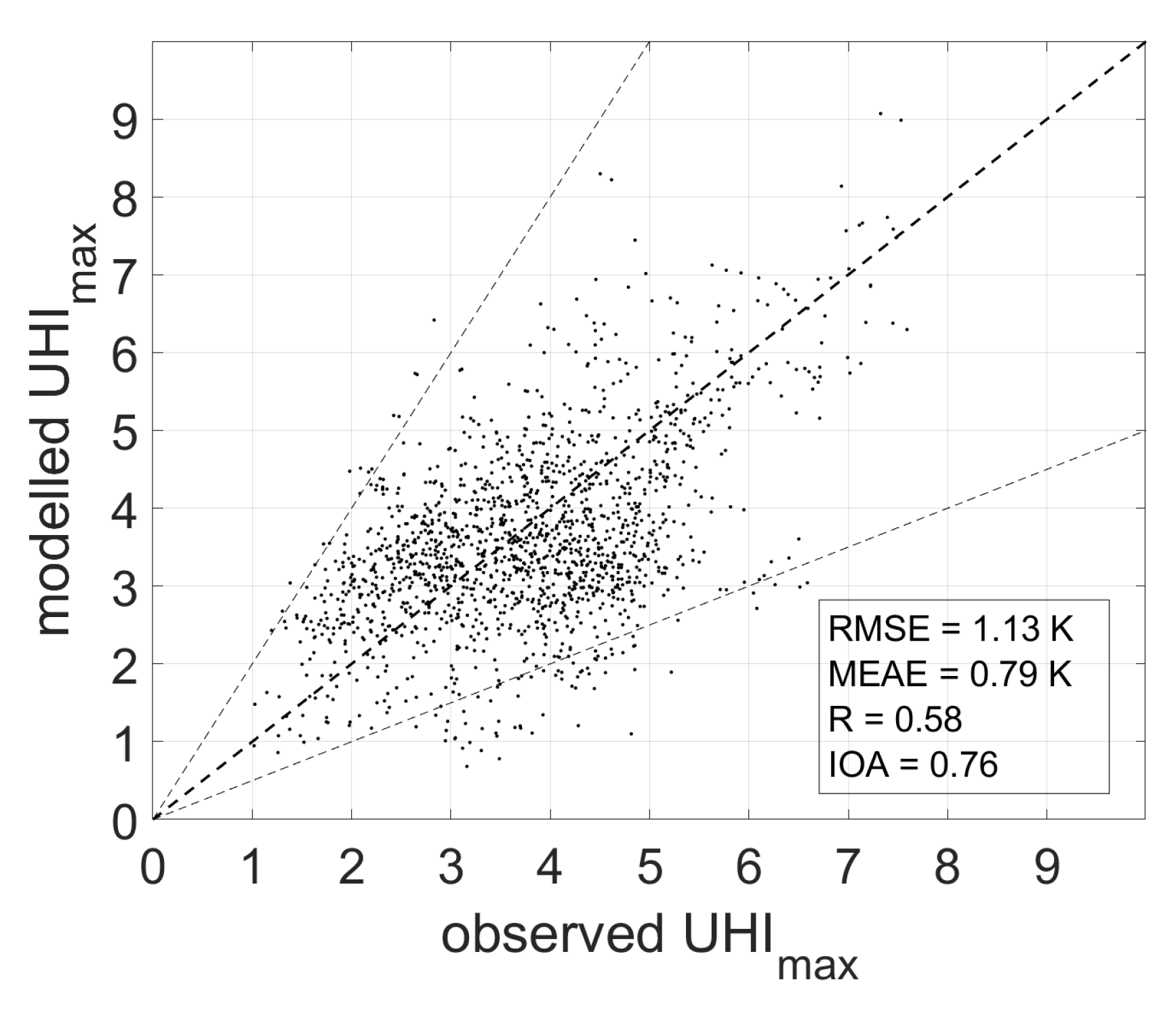
• Evaluation of the model adapted to Singapore (Equation (3)) shows overall good agreement with observations of daily UHI_max for different dry weather conditions.
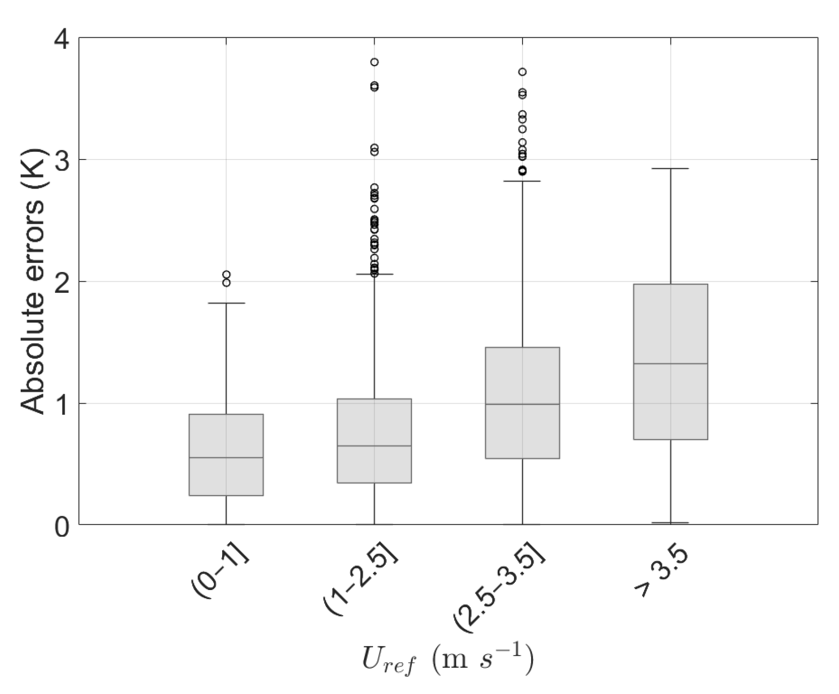
• Model performance shows a strong dependency of the estimated UHI_max on wind speed. Best performance is reached for low wind speed (<2.5 m s⁻¹ at the reference site). During these conditions, the model provides reliable estimations of UHI_max with low errors (RMSE and MEAE < 1 K) and a high level of agreement with observations (R > 0.80).
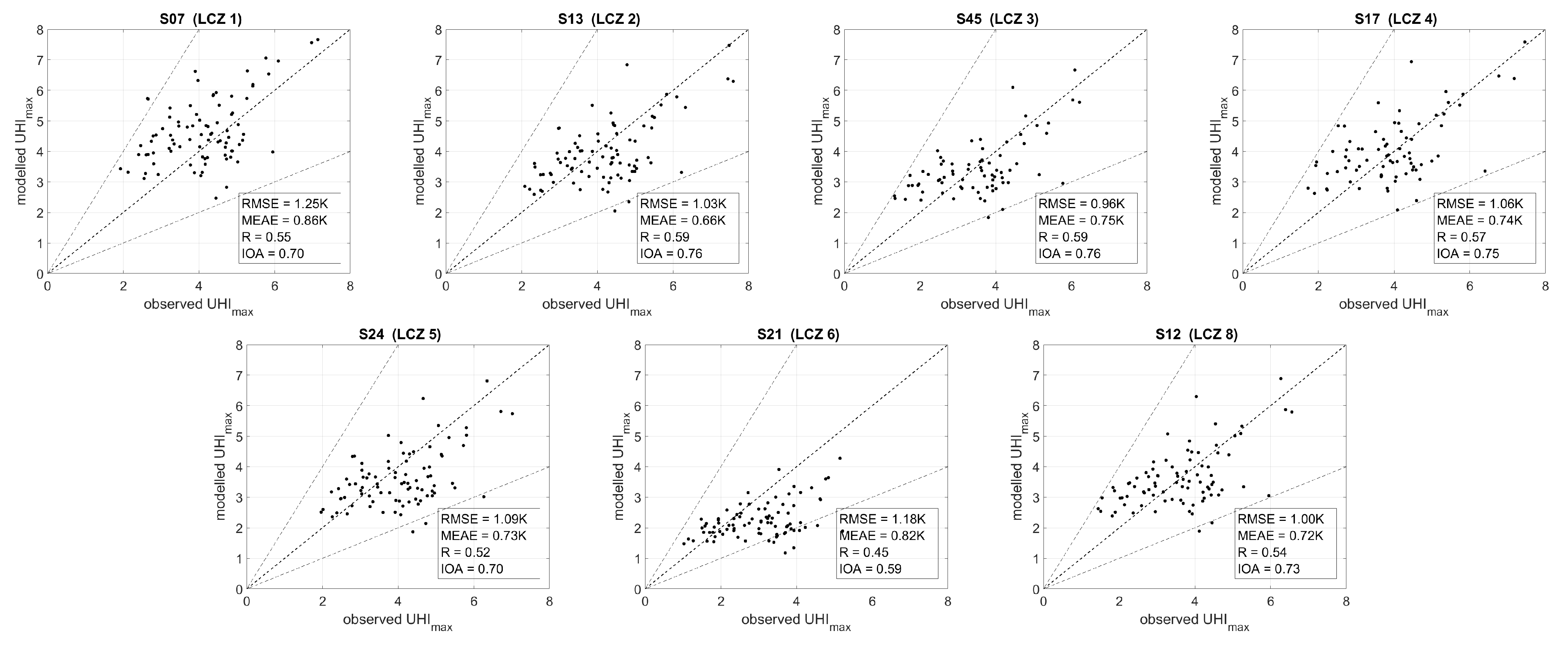
• Estimates for UHI_max tend to underpredict observed values over open low-rise areas (LCZ 6) (R < 0.5). The paucity of stations with low $F_{urb}$ values (0.3–0.6), compared to the majority of stations that are placed in more densely built-up environments ($F_{urb}$ > 0.6), is one reason why the model is less robust over these open urban landscapes. Given nevertheless significant UHI_max magnitudes over less developed urban spaces, we suggest increasing the placement of stations in these areas.
• The low prediction errors (RMSE < 1.2 K and MEAE < 1 K) obtained at every station and for different seasons in Singapore reveal that the accuracy of this simple semi-empirical equation might be comparable to the performance for dry weather conditions of more sophisticated numerical models (e.g., WRF or uSINGV), which include complex building effect parameterizations.

The present model serves as a reliable and easy-to-use tool to calculate the spatial variability of UHI_max intensity across the tropical city of Singapore. However, there is still potential for improvement. Although the spatial performance of the estimated UHI_max is consistent with the expected results according to the LCZ classification, the model should also be evaluated at different measurement points from the locations used to build the equation in order to confirm its accuracy across the entire city. Additional improvements might be incorporated for even better performance, e.g., the inclusion of other factors known to influence the UHI, such as local anthropogenic heat fluxes. The latter would particularly improve the estimation of UHI_max magnitudes in areas known to have high anthropogenic heat emissions, such as certain industrial estates or commercial centers with dense building configurations and high traffic volumes.

As with all such approaches, the present semi-empirical model is fundamentally restricted by the statistical relationships between parameters established for the present situation. However, the model has descriptive and practical value by providing UHI_max maps that are easy to calculate based on a few input variables. The present semi-empirical equation performs best during calm wind conditions, which coincides with maximum UHI development and highest UHI_max values. This is an important result as these situations are associated with reduced outdoor thermal comfort and higher health risk. Hence, the resulting maps can be used to investigate less favorable thermal conditions and assess the population vulnerability to a certain temperature excess and thus identify risk levels of a target region [51]. Additionally, the spatial distribution of the modeled UHI_max can provide insights for urban planning strategies [52], as well as for designing corresponding mitigation measures according to the land cover and morphology of a location.

References

1. Stewart, I.D. Why should urban heat island researchers study history? Urban Clim. 2019, 30, 100484. [Google Scholar] [CrossRef]
2. Oke, T.R.; Mills, G.; Christen, A.; Voogt, J.A. Urban Climates; Cambridge University Press: Cambridge, UK, 2017. [Google Scholar] [CrossRef]
3. Rizwan, A.M.; Dennis, L.Y.; Chunho, L. A review on the generation, determination and mitigation of Urban Heat Island. J. Environ. Sci. 2008, 20, 120–128. [Google Scholar] [CrossRef] [PubMed]
4. Steeneveld, G.J.; Koopmans, S.; Heusinkveld, B.; Van Hove, L.; Holtslag, A. Quantifying urban heat island effects and human comfort for cities of variable size and urban morphology in the Netherlands. J. Geophys. Res. Atmos. 2011, 116, D20. [Google Scholar] [CrossRef]
5. Schatz, J.; Kucharik, C.J. Seasonality of the urban heat island effect in Madison, Wisconsin. J. Appl. Meteorol. Climatol. 2014, 53, 2371–2386. [Google Scholar] [CrossRef]
6. Oke, T.R. The urban energy balance. Prog. Phys. Geogr. 1988, 12, 471–508. [Google Scholar] [CrossRef]
7. Oke, T.R. Canyon geometry and the nocturnal urban heat island: Comparison of scale model and field observations. J. Climatol. 1981, 1, 237–254. [Google Scholar] [CrossRef]
8. Unger, J. Intra-urban relationship between surface geometry and urban heat island: Review and new approach. Clim. Res. 2004, 27, 253–264. [Google Scholar] [CrossRef]
9. Yuan, C.; Chen, L. Mitigating urban heat island effects in high-density cities based on sky-view factor and urban morphological understanding: A study of Hong Kong. Archit. Sci. Rev. 2011, 54, 305–315. [Google Scholar] [CrossRef]
10. Zoulia, I.; Santamouris, M.; Dimoudi, A. Monitoring the effect of urban green areas on the heat island in Athens. Environ. Monit. Assess. 2009, 156, 275–292. [Google Scholar] [CrossRef]
11. Oliveira, S.; Andrade, H.; Vaz, T. The cooling effect of green spaces as a contribution to the mitigation of urban heat: A case study in Lisbon. Build. Environ. 2011, 46, 2186–2194. [Google Scholar] [CrossRef]
12. Konarska, J.; Holmer, B.; Lindberg, F.; Thorsson, S. Influence of vegetation and building geometry on the spatial variations of air temperature and cooling rates in a high-latitude city. Int. J. Climatol. 2016, 36, 2379–2395. [Google Scholar] [CrossRef]
13. Freitas, E.D.; Rozoff, C.M.; Cotton, W.R.; Dias, P.L.S. Interactions of an urban heat island and sea-breeze circulations during winter over the metropolitan area of São Paulo, Brazil. Bound.-Layer Meteorol. 2007, 122, 43–65. [Google Scholar] [CrossRef]
14. He, B.J.; Ding, L.; Prasad, D. Relationships among local-scale urban morphology, urban ventilation, urban heat island and outdoor thermal comfort under sea breeze influence. Sustain. Cities Soc. 2020, 60, 102289. [Google Scholar] [CrossRef]
15. Skarbit, N.; Stewart, I.D.; Unger, J.; Gál, T. Employing an urban meteorological network to monitor air temperature conditions in the ‘local climate zones’ of Szeged, Hungary. Int. J. Climatol. 2017, 37, 582–596. [Google Scholar] [CrossRef]
16. Stewart, I.D. A systematic review and scientific critique of methodology in modern urban heat island literature. Int. J. Climatol. 2011, 31, 200–217. [Google Scholar] [CrossRef]
17. Arnds, D.; Böhner, J.; Bechtel, B. Spatio-temporal variance and meteorological drivers of the urban heat island in a European city. Theor. Appl. Climatol. 2017, 128, 43–61. [Google Scholar] [CrossRef]
18. Giannaros, T.M.; Melas, D.; Daglis, I.A.; Keramitsoglou, I.; Kourtidis, K. Numerical study of the urban heat island over Athens (Greece) with the WRF model. Atmos. Environ. 2013, 73, 103–111. [Google Scholar] [CrossRef]
19. Chen, F.; Yang, X.; Zhu, W. WRF simulations of urban heat island under hot-weather synoptic conditions: The case study of Hangzhou City, China. Atmos. Res. 2014, 138, 364–377. [Google Scholar] [CrossRef]
20. Yang, B.; Zhang, Y.; Qian, Y. Simulation of urban climate with high-resolution WRF model: A case study in Nanjing, China. Asia-Pac. J. Atmos. Sci. 2012, 48, 227–241. [Google Scholar] [CrossRef]
21. Salamanca, F.; Martilli, A.; Yagüe, C. A numerical study of the Urban Heat Island over Madrid during the DESIREX (2008) campaign with WRF and an evaluation of simple mitigation strategies. Int. J. Climatol. 2012, 32, 2372–2386. [Google Scholar] [CrossRef]
22. Gutiérrez, E.; González, J.E.; Martilli, A.; Bornstein, R.; Arend, M. Simulations of a heat-wave event in New York City using a multilayer urban parameterization. J. Appl. Meteorol. Climatol. 2015, 54, 283–301. [Google Scholar] [CrossRef]
23. Li, H.; Zhou, Y.; Wang, X.; Zhou, X.; Zhang, H.; Sodoudi, S. Quantifying urban heat island intensity and its physical mechanism using WRF/UCM. Sci. Total Environ. 2019, 650, 3110–3119. [Google Scholar] [CrossRef] [PubMed]
24. Kusaka, H.; Chen, F.; Tewari, M.; Dudhia, J.; Gill, D.O.; Duda, M.G.; Wang, W.; Miya, Y. Numerical simulation of urban heat island effect by the WRF model with 4-km grid increment: An inter-comparison study between the urban canopy model and slab model. J. Meteorol. Soc. Jpn. 2012, 90, 33–45. [Google Scholar] [CrossRef]
25. Sharma, A.; Fernando, H.J.; Hamlet, A.F.; Hellmann, J.J.; Barlage, M.; Chen, F. Urban meteorological modeling using WRF: A sensitivity study. Int. J. Climatol. 2017, 37, 1885–1900. [Google Scholar] [CrossRef]
26. Bottyán, Z.; Unger, J. A multiple linear statistical model for estimating the mean maximum urban heat island. Theor. Appl. Climatol. 2003, 75, 233–243. [Google Scholar] [CrossRef]
27. Hoffmann, P.; Krueger, O.; Schlünzen, K.H. A statistical model for the urban heat island and its application to a climate change scenario. Int. J. Climatol. 2012, 32, 1238–1248. [Google Scholar] [CrossRef]
28. Straub, A.; Berger, K.; Breitner, S.; Cyrys, J.; Geruschkat, U.; Jacobeit, J.; Kuehlbach, B.; Kusch, T.; Philipp, A.; Schneider, A.; et al. Statistical modelling of spatial patterns of the urban heat island intensity in the urban environment of Augsburg, Germany. Urban Clim. 2019, 29, 100491. [Google Scholar] [CrossRef]
29. Gardes, T.; Schoetter, R.; Hidalgo, J.; Long, N.; Marquès, E.; Masson, V. Statistical prediction of the nocturnal urban heat island intensity based on urban morphology and geographical factors—An investigation based on numerical model results for a large ensemble of French cities. Sci. Total Environ. 2020, 737, 139253. [Google Scholar] [CrossRef] [PubMed]
30. Buckingham, E. On Physically Similar Systems; Illustrations of the Use of Dimensional Equations. Phys. Rev. 1914, 4, 345–376. [Google Scholar] [CrossRef]
31. Hidalgo, J.; Masson, V.; Gimeno, L. Scaling the daytime urban heat island and urban-breeze circulation. J. Appl. Meteorol. Climatol. 2010, 49, 889–901. [Google Scholar] [CrossRef]
32. Lee, T.W.; Lee, J.; Wang, Z.H. Scaling of the urban heat island intensity using time-dependent energy balance. Urban Clim. 2012, 2, 16–24. [Google Scholar] [CrossRef]
33. Theeuwes, N.E.; Steeneveld, G.J.; Ronda, R.J.; Holtslag, A.A. A diagnostic equation for the daily maximum urban heat island effect for cities in northwestern Europe. Int. J. Climatol. 2017, 37, 443–454. [Google Scholar] [CrossRef]
34. Zhang, X.; Steeneveld, G.J.; Zhou, D.; Duan, C.; Holtslag, A.A. A diagnostic equation for the maximum urban heat island effect of a typical Chinese city: A case study for Xi’an. Build. Environ. 2019, 158, 39–50. [Google Scholar] [CrossRef]
35. Yao, L.; Yang, X.; Zhu, C.; Jin, T.; Peng, L.L.; Ye, Y. Evaluation of a Diagnostic equation for the daily maximum urban heat island effect. Procedia Eng. 2017, 205, 2863–2870. [Google Scholar] [CrossRef]
36. Yang, X.; Yao, L.; Peng, L.L.; Jiang, Z.; Jin, T.; Zhao, L. Evaluation of a diagnostic equation for the daily maximum urban heat island intensity and its application to building energy simulations. Energy Build. 2019, 193, 160–173. [Google Scholar] [CrossRef]
37. Chow, W.T.; Roth, M. Temporal dynamics of the urban heat island of Singapore. Int. J. Climatol. J. R. Meteorol. Soc. 2006, 26, 2243–2260. [Google Scholar] [CrossRef]
38. Jin, H.; Cui, P.; Wong, N.H.; Ignatius, M. Assessing the effects of urban morphology parameters on microclimate in Singapore to control the urban heat island effect. Sustainability 2018, 10, 206. [Google Scholar] [CrossRef]
39. Roth, M.; Sanchez, B.; Li, R.; Velasco, E. Spatial and temporal characteristics of near-surface air temperature across local climate zones in a tropical city. Int. J. Climatol. 2022, 42, 9730–9752. [Google Scholar] [CrossRef]
40. Mughal, M.O.; Li, X.X.; Yin, T.; Martilli, A.; Brousse, O.; Dissegna, M.A.; Norford, L.K. High-resolution, multilayer modeling of Singapore’s urban climate incorporating local climate zones. J. Geophys. Res. Atmos. 2019, 124, 7764–7785. [Google Scholar] [CrossRef]
41. DOS. Yearbook of Statistics Singapore 2019; Department of Statistics (DOS), Ministry of Trade & Industry: Singapore, 2019.
42. Stewart, I.D.; Oke, T.R. Local climate zones for urban temperature studies. Bull. Am. Meteorol. Soc. 2012, 93, 1879–1900. [Google Scholar] [CrossRef]
43. Gorelick, N.; Hancher, M.; Dixon, M.; Ilyushchenko, S.; Thau, D.; Moore, R. Google Earth Engine: Planetary-scale geospatial analysis for everyone. Remote Sens. Environ. 2017, 202, 18–27. [Google Scholar] [CrossRef]
44. Demuzere, M.; Bechtel, B.; Mills, G. Global transferability of local climate zone models. Urban Clim. 2019, 27, 46–63. [Google Scholar] [CrossRef]
45. Middel, A.; Lukasczyk, J.; Maciejewski, R.; Demuzere, M.; Roth, M. Sky View Factor footprints for urban climate modeling. Urban Clim. 2018, 25, 120–134. [Google Scholar] [CrossRef]
46. Simón-Moral, A.; Dipankar, A.; Roth, M.; Sánchez, C.; Velasco, E.; Huang, X.Y. Application of MORUSES single-layer urban canopy model in a tropical city: Results from Singapore. Q. J. R. Meteorol. Soc. 2020, 146, 576–597. [Google Scholar] [CrossRef]
47. Li, R. Spatio-Temporal Dynamics of the Urban Heat Island in Singapore. Master’s Thesis, Department of Geography, National University of Singapore, Singapore, 2012. [Google Scholar]
48. Yow, D.M. Urban heat islands: Observations, impacts, and adaptation. Geogr. Compass 2007, 1, 1227–1251. [Google Scholar] [CrossRef]
49. Runnalls, K.; Oke, T. Dynamics and controls of the near-surface heat island of Vancouver, British Columbia. Phys. Geogr. 2000, 21, 283–304. [Google Scholar] [CrossRef]
50. Sanchez, B.; Roth, M.; Simón-Moral, A.; Martilli, A.; Velasco, E. Assessment of a meteorological mesoscale model’s capability to simulate intra-urban thermal variability in a tropical city. Urban Clim. 2021, 40, 101006. [Google Scholar] [CrossRef]
51. Zhu, W.; Yuan, C. Urban heat health risk assessment in Singapore to support resilient urban design—By integrating urban heat and the distribution of the elderly population. Cities 2023, 132, 104103. [Google Scholar] [CrossRef]
52. Koopmans, S.; Ronda, R.; Steeneveld, G.J.; Holtslag, A.A.; Klein Tank, A.M. Quantifying the effect of different urban planning strategies on heat stress for current and future climates in the agglomeration of The Hague (The Netherlands). Atmosphere 2018, 9, 353. [Google Scholar] [CrossRef]
Figure 1. Location of five MSS weather stations (diamond) and 26 air temperature sensors at 2–3 m height, of which 24 are placed in urban areas (dots) and two in rural areas with scattered trees (triangle). Background image: LCZ map from Middel et al. [45].
Sustainability 15 12834 g001
Figure 2. (a) Modeled UHImax applying Equation (1) against observed UHImax from 19 urban stations for dry days. (b) Relationship between observed UHImax and DTRrur at Station S41 for dry days.
Sustainability 15 12834 g002
Figure 3. Observed mean UHImax at 24 urban stations for dry days against: (a) urban fraction ( F u r b ), (b) vegetation fraction ( F v e g ), (c) street aspect ratio (H/W) and (d) local sky-view factor (SVF). Vertical lines denote +/−1 standard deviation.
Sustainability 15 12834 g003
Figure 4. Relationship between: (a) UHImax (K), T a , r e f (K), and T d , r e f (K), and (b) T a , r e f (K), T d , r e f (K) and U r e f (m s−1) for S41 for dry days.
Sustainability 15 12834 g004
Figure 5. Relationship between the two dimensionless groups plotted as log( Π 2 ) against log( Π 1 ) for two examples, stations S07 (black) and S41 (red) and the respective linear trend lines.
Sustainability 15 12834 g005
Figure 6. Scatter plots of the estimated α for each station i ( α i ) against (a) F u r b , (b) 1 1 1 + H / W , and (c) the function a · F u r b + b · 1 1 1 + H / W , where a and b are obtained using the multiple linear regression method and are 0.9 and 0.5, respectively.
Sustainability 15 12834 g006
Figure 7. Modeled (using Equation (3)) against observed UHImax for 24 stations and for the second subset of the data (91 nights). Dashed lines indicate the 1:1 relationship and the range of factor of two (FAC2).
Sustainability 15 12834 g007
Figure 8. Same as Figure 7 for S07 (LCZ 1), S13 (LCZ 2), S45 (LCZ 3), S17 (LCZ 4), S24 (LCZ 5), S21 (LCZ 6), and S25 (LCZ 8).
Sustainability 15 12834 g008
Figure 9. Absolute errors in UHImax (= | UHI max , modeled UHI max , observed | ) as a function of reference wind speed regime for the test dataset (91 nights). The box defines the interquartile range (IQR), the horizontal line is the median, whiskers extend to 1.5 times the IQR, and circles are outliers.
Sustainability 15 12834 g009
Figure 10. (a) Mean UHImax map using Equation (3) applied to 300 m gridded morphological data for ideal conditions (36 nights), (b) scatter plot of modeled and observed mean UHImax for the 24 urban stations, and (c) spatial average of modeled mean UHImax for ideal nights according to the urban LCZ types.
Sustainability 15 12834 g010
Figure 11. Maps for the (a) lowest UHImax intensity observed on 5 February 2012, (b) highest UHImax observed on 19 June 2013, (c) mean UHImax map for dry days in February, and (d) mean UHImax map for dry days in June within the study period.
Sustainability 15 12834 g011