Seismic Response of Earth-Rock Dams with Innovative Antiseepage Walls on the Effect of Microscopic Fluid-Solid Coupling

Abstract

In dykes and dam projects, the microscopic fluid-solid coupling effect from the interaction between soil skeleton and pore water during an earthquake is crucial to consider, as it can lead to dam safety problems. To control seepage in medium- and small-sized dams, polymer antiseepage walls have emerged as effective measures. In recent years, this method has been increasingly utilized in projects worldwide as it is essential for preventing potential dam safety issues. To address concerns related to seismic safety, this study conducts theoretical analysis, model tests, and numerical simulations to investigate the seismic response of earth-rock dams with polymer antiseepage walls, with a specific focus on the microscopic fluid-solid coupling effect. The dynamic viscoelastic constitutive model used in this study incorporates Biot’s theory of dynamic consolidation and the results of dynamic mechanical analysis (DMA) of polymer materials. To validate the model, a centrifuge test is performed, and it is then utilized to study the seismic response of earth-rock dams with polymer antiseepage walls. Furthermore, the influence of factors such as fluid-solid coupling, water level, polymer material density, and wall thickness on the seismic response of dams with antiseepage walls is analyzed. Finally, the seismic safety of the earth-rock dam with the polymer antiseepage wall is thoroughly examined. The results emphasize the need to consider the fluid-solid coupling effect, as factors like water level and design parameters of the antiseepage wall significantly impact the seismic response of earth-rock dams with polymer antiseepage walls.

1. Introduction

In the context of modern engineering and infrastructure development, sustainability principles have become paramount to ensuring a harmonious coexistence between human progress and being environmentally friendly. Recently, there has been a rise in the use of innovative non-water-reacted polymer materials for constructing antiseepage walls in dam reinforcement and emergency rescue projects [1]. This material is preferred due to its lightweight nature, non-polluting characteristics, excellent anti-seepage performance, and outstanding durability [2,3]. Figure 1 presents a schematic diagram that illustrates the material synthesis process, specialized grouting equipment, and construction methods.

A special hole-drilling tool with static pressing equipment is used during the construction of antiseepage walls to penetrate the dam and create a continuous ultra-thin slot [4] Following this, a two-component polymer material is injected into the slot through a grouting pipe, initiating a chemical reaction. This reaction causes the combined materials to rapidly expand, effectively filling the slot and solidifying into polymer plates [5]. Eventually, the adjacent hole plates bond together, forming a continuous ultra-thin polymer wall. This process significantly enhances the dam’s antiseepage performance [6]. The adoption of polymer material not only addresses dam safety concerns but also aligns with the broader goals of sustainable development. By mitigating seepage in medium and small-sized dams, these antiseepage walls contribute to enhanced infrastructure performance while minimizing environmental impact [7].

Numerous dam failures have been triggered by earthquakes. For instance, the collapse of the Tangjiashan dam occurred after the Wenchuan earthquake in 2008 [8], the Fujinuma dam was damaged following the Tōhoku earthquake in 2011 [9], the Fundão mine tailings dam was broken after the southeastern Brazil earthquake in 2015 [10], and the landslides and dam damage were caused by the Jiuzhaigou earthquake in 2017 [11]. During earthquakes, earth-rock dams experience dynamic fluid-solid coupling effects, which refer to the transfer of stress (pore pressure) between the pore water and soil skeleton within the dams [12]. This coupling effect results in deformation and potential damage. Notably, under strong earthquakes, the impact of this coupling effect becomes more pronounced, causing various safety concerns for dams. These concerns include the formation of cracks, landslides, permanent deformation, liquefaction, and even the risk of dam break [13], as shown in Figure 2.

This study investigates the seismic response of earth-rock dams with polymer anti-seepage walls. Two types of dynamic fluid-solid coupling effects [14] can be identified between earth-rock dams and reservoir water under seismic conditions. The first type is the macroscopic fluid-solid coupling effect that occurs at the interface between the reservoir water and the dam. At this interface, the water and dam are clearly separated on a macroscopic scale. The second type is the microscopic fluid-solid coupling effect that occurs within the earth-rock dams. Within the dam, the water and soil cannot be distinguished on a macroscopic scale. The focus of this study is the second type of coupling effect, which involves the microscopic interaction between the soil skeleton and pore water.

For interpreting the microscopic fluid-solid coupling effect between the soil skeleton and pore water, Terzaghi [15] first proposed the concept of effective stress in 1925 and combined it with Darcy’s law to create the soil consolidation theory. This theory was suitable for solving one-dimensional soil consolidation cases but not strictly applicable in two- and three-dimensional cases. Biot then developed a more accurate three-dimensional quasi-static consolidation equation and laid the groundwork for static fluid-solid coupling theory. This theory applied Terzaghi’s principle and continuum theory to fluid and solid media and explained how soil skeleton and pore water are coupled in soil mass. In 1956, Biot [16] developed the dynamic consolidation theory based on the static consolidation equation, taking into account the inertia force of the soil skeleton and pore water. This theory, which is derived from Biot’s theory, could be used to compute the coupling impact of the soil skeleton and pore water under dynamic conditions. Biot’s theory is more effective at describing microscopic dynamic fluid-solid coupling than early theories. As a result, numerous studies have been conducted using Biot’s dynamic consolidation hypothesis. Lin et al. [17] used Biot’s theory to investigate fluid wave response in porous media. They used the sandstone test to determine the link between linear porosity and modulus and then to derive the parameters for Biot’s dynamic consolidation equation. Ghaboussi et al. [18,19] established a finite element method by using the variational principle based on Biot’s theory. Using finite element analysis, the dynamic response and liquefaction [20] of layered sand under seismic response were investigated. Zienkiewicz et al. [21,22,23] continued to research Biot’s dynamic consolidation theory and simplified the equation in accordance with various unknowns. They rewrote it into four different forms: “u-p” form, “u-w” form, “u-U” form, and “u-w-p” form. Pan [24], Liu [25], and Chen [26] explored dam-foundation-reservoir interactions, highlighting the impact of foundation size and dam foundation dynamics on dam acceleration. Kong [27] proposed a spectral element-based numerical method for fluid-solid seismic wave interactions. Zhang [28] bridged wavefield simulation and dam seismic analysis. Rayegani [29,30] stressed the need for advanced strategies like intelligent dampers to enhance dam seismic resistance. Jing [31] compared near-field and far-field seismic wave effects on earth-rock dams, enriching our understanding of complex interactions. These theories and methods provide new approaches for studying the dynamic coupling effect between pore water and earth-rock dams under seismic action and contribute to investigating the dynamic coupling effect of pore water and earth-rock dams under earthquake action.

Based on the aforementioned review, the polymer antiseepage wall has been widely used in the reinforcement projects of earth-rock dams as a new type of antiseepage wall. However, there are limitations in the current understanding of its dynamic interaction with the soil skeleton and pore water. Although studies have been conducted on the static fluid-solid coupling of polymer antiseepage walls in earth-rock dams, the dynamic fluid-solid coupling model based on Biot’s static consolidation theory is insufficient for fully describing this dynamic interaction. Therefore, it is of high significance to adopt a coupling theory that accurately represents the fine-scale fluid-solid coupling effect in the seismic response analysis of earth-rock dams to establish a fully coupled dynamic model that incorporates the fluid-solid interaction. In this study, based on Biot’s dynamic consolidation theory, a static and dynamic finite differential model of the earth-rock dam with a polymer antiseepage wall was developed to examine the effect of microscopic fluid-solid coupling. To reflect the material properties in the model, a dynamic viscoelastic constitutive model of polymer materials was developed using DMA test results. The numerical model was then validated by centrifuge test data [32] and the seismic response laws of antiseepage walls [33] were studied. Furthermore, the response of an earth-rock dam with a concrete antiseepage wall was also investigated for comparison. Finally, the seismic stability of the earth-rock dam with a polymer antiseepage wall was analyzed, and the related mechanisms were discussed.

2. Theory and Model

2.1. Theoretical Research

Biot’s dynamic consolidation equation is utilized to describe the microscopic dynamic fluid-solid coupling effect between the soil skeleton and pore space. Biot’s dynamic consolidation equation serves as the coupling equation, and its solution is obtained using the finite difference method [34]. The following assumptions are proposed to make the derivation of Biot’s dynamic consolidation theory [35,36,37]:

• Soil skeleton is an ideal continuous porous medium, of which compressibility is ignored;
• Pore water is compressible and its flow obeys the generalized Darcy’s law;
• Soils are isotropic medium and pores are interconnected;
• Pore size is much smaller than the seimic wavelength;
• The effect of temperature is ignored.

Considering the compressibility of soil particles, the revised effective stress is as follow [38]:

$${\sigma }_{ij}^{″}={\sigma }_{ij}^{\mathrm{\prime }}={\sigma }_{ij}+\alpha {\delta }_{ij}p,$$

(1)

In the formula, ${\sigma }_{ij}$ is the total stress, ${\delta }_{ij}$ is the Kronecker function, $p$ is the pore water pressure, $\alpha$ is the Biot’s constant, $\alpha$ = 1 − Kb/Ks; Kb and Ks are soil skeleton and soil particles of the bulk modulus, and the value of α is 1, assuming the soil particles being incompressible.

The Mohr-Coulomb model is chosen as the constitutive model for the analysis. To ensure the accuracy of the software analysis, the fatigue behavior of the soil was not considered in this model. The total deformation consists of two parts: elastic deformation and plastic deformation.

The elastic deformation is represented by Hooke’s law:

$${\sigma }_{ij}=2\mu {\epsilon }_{ij}+\lambda {\epsilon }_{kk}{\delta }_{ij}-\alpha {\delta }_{ij}p,$$

(2)

In the formula, $\lambda$ and $\mu$ are Lame constants, $\lambda =\frac{Ev}{\left(1+v\right)\left(1-2v\right)}$,$\mu =\frac{E}{2\left(1+v\right)}$, ${\epsilon }_{ij}$ is the strain rate of soil skeleton, and ${\epsilon }_{kk}$ is the volumetric strain, ${\epsilon }_{kk}={\epsilon }_{11}+{\epsilon }_{22}+{\epsilon }_{33}$.

The plastic deformation is represented by the yield criterion of the Mohr-Coulomb model:

$${\tau }_n={\sigma }_{n}tg\phi +c$$

(3)

In the formula, $c,\phi$ are the cohesion and angle of internal friction of the material.

The motion of the fluid is expressed by Darcy’s law:

$$q_i=-k_{ij}\widehat{k}\left(s\right)\left(p-{\rho }_f{x}_i{g}_i\right)$$

(4)

In the formula, $k_{ij}$ is the dynamic permeability coefficient, $k_{ij}=k/\rho g$,$k$ is the permeability coefficient in soil mechanics, and $\widehat{k}\left(s\right)$ is the coefficient related to fluid saturation.

The equilibrium equations include momentum balance equation and fluid mass balance equation. Momentum balance equation is listed as follows:

$${\sigma }_{ij,j}+\rho g_i-\rho {\ddot{u}}_i=0$$

(5)

In the formula, ${\ddot{u}}_i$ is the acceleration of soil skeleton, ρ is the total effective density, $\rho =n{\rho }_f+\left(1-n\right){\rho }_s$,${\rho }_f$ is the density of water, ${\rho }_s$ is the density of soil skeleton, and $g_i$ is the acceleration of gravity.

The fluid mass balance equation is listed as follows:

$$-q_{i,j}+q_v=\frac{\partial \zeta }{\partial t}$$

(6)

In the formula, $q_{i,j}$ is the velocity of fluid seepage, $q_{i,j}=\frac{\partial q_i}{\partial x_i}=\frac{\partial q_i}{\partial x}+\frac{\partial q_i}{\partial y}$,$q_v$ is the inflow of liquid per unit time, and $\zeta$ is the change of the fluid volume in the porous media per unit volume.

The constitutive equation of pore fluid is listed as follows:

$$\frac{1}{M}\frac{\partial p}{\partial t}+\frac{n}{s}\frac{\partial s}{\partial t}=\frac{1}{s}\frac{\partial \zeta }{\partial t}-\alpha \frac{\partial \epsilon }{\partial t}$$

(7)

In the formula, M is Biot’s modulus and $\epsilon$ is the volumetric strain of soil mass.

Substituting the fluid mass balance equation into the pore fluid’s continuity equation, the expression for the fluid continuity equation is obtained:

$$\frac{1}{M}\frac{\partial p}{\partial t}+\frac{n}{s}\frac{\partial s}{\partial t}=\frac{1}{s}\left(-q_{i,j}+q_v\right)-\alpha \frac{\partial \epsilon }{\partial t}$$

(8)

Substituting Darcy’s law into the fluid continuity equation and assuming the soil saturation being 1:

$${\left[k_{ij}\left(-p+{\rho }_f{g}_i\right)\right]}_j-q_v+\alpha \frac{\partial \epsilon }{\partial t}+\frac{1}{M}\frac{\partial p}{\partial t}=0$$

(9)

2.2. Static Fluid-Solid Coupling Model

In this paper, a static fluid-solid coupling model for earth-rock dam with polymer antiseepage wall was established, taking the earth-rock dam of Jiulong Reservoir as the prototype.

2.2.1. Model Building

The earth-rock dam of Jiulong Reservoir is a small dam situated in Jiulong River, Luoshan County, Xinyang City, Henan Province, China. The materials of the dam’s body and foundation are mainly composed of heavy silty soil with an average permeability coefficient of 2.6 × 10⁻⁵ cm/s. The dam is 15 m tall, 240 m long, 5.6 m wide at its top, and 90 m wide at its bottom. The earth-rock dam needed to be strengthened as there were significant leak problems after operating for 60 years. So a polymer antiseepage wall with a thickness of 0.03 m was constructed in the dam for reinforcement. The wall is 2 m deep into the dam’s base, with a total length of 215 m along the dam’s axis, as shown in Figure 3a.

The FLAC3D 7.0 software was used for the analysis. The dimensions of the earth-rock dam model were the same as the prototype, with a width of 189.6 m and a dam base height of 15 m. The dam was evenly distributed along the dam axis direction, and the upstream water level was 8.6 m. To improve calculation efficiency, the model was set to unit thickness. An antiseepage wall, located 0.5 m away from the dam axis line on the upstream dam slope, was added inside the earth-rock dam. The wall had a height of 17 m, extending 2 m into the dam base, and a thickness of 0.03 m. The cross-section of the earth-rock dam with a polymer antiseepage wall is depicted in Figure 3b. The grid in the antiseepage wall area was densified, while the partitioned grid met the requirements for conducting seismic analysis. For the continuity of hydrostatic calculation, the numerical model was divided into 3505 units and 7400 nodes. Hexahedral computational elements were used for calculations, as seen in Figure 3c.

2.2.2. Boundary Conditions

In fluid-soil coupling analysis, the boundary conditions consist of a stress boundary, a displacement boundary, a flow potential boundary, and a flow boundary. The fixed boundaries are applied to the bottom of the dam foundation to restrict movement in three directions. The horizontal displacement and displacement along the dam axis direction are constrained by the left and right sides of the dam foundation, respectively. The upstream reservoir water exerts stress and seepage in the stress field and seepage field of the earth-rock dam. On the upstream slope and the foundation surface, it applies hydrostatic pressure and pore water pressure. Additionally, a drainage boundary with a value of 0 is set as the flow boundary on the right side of the dam foundation. In addition to considering stress and displacement boundaries, the movement of pore water relative to the soil skeleton, i.e., pore water pressure boundary and fluid flow boundary conditions, also needs to be considered. The boundary conditions of the fluid-solid coupling earth-rock dam model with a polymer antiseepage wall are as follows:

Displacement boundary:

$$u_i=u_{i0}$$

(10)

Stress boundary:

$${\sigma }_{ij}=t_{i0}$$

(11)

Flow potential boundary:

$$P=P_0$$

(12)

Flow boundary:

$$-k_n=\frac{\partial p}{\partial n}=q_0$$

(13)

In the numerical analysis, the Mohr-Coulomb elastoplastic constitutive model is selected for soils, the linear elastic constitutive model is for concrete, and the generalized Maxwell constitutive model is for viscoelastic polymer materials.

For comparison, the dam model with a concrete antiseepage wall was established with a thickness of 0.5 m. Other geometric parameters are the same as those of the polymer antiseepage wall. The parameters of materials are shown in

Table 1. Mechanical parameters of materials.

	Young’s Modulus (Pa)	Density (kg/m3)	Poisson Ratio	Permeability Coefficient (m/s)	Porosity	Cohesion (Pa)	Internal Friction Angle (°)
Soil	3.72 × 107	2000	0.35	2.3 × 10−7	0.3	2.22 × 104	11.3
Polymer-I	1.80 × 107	160	0.18	10−9	-	-	-
polymer-II	2.00 × 107	260	0.20	10−9	-	-	-
polymer-III	1.09 × 108	350	0.22	10−9	-	-	-
Concrete	2.00 × 109	2400	0.20	2.6 × 10−9	-	-	-

[39].

Darcy’s law generally meets the seepage condition of a dam while an initial hydraulic gradient exists. The boundary condition of the known water head is represented by the contact surface (Γ) between the dam body and the polymer wall, listed as follows:

$$h_c\left(x_i,t\right)\left|{\Gamma }_1\right.=h_{c1}\left(x_i,t\right)$$

(14)

Under seismic reaction, the contact surface ($\Gamma$) between the dam body and the polymer wall should also meet the following boundary condition.

$$\frac{\partial p}{\partial n}=-\rho {\ddot{u}}_n$$

(15)

In the formula, p is the pore water pressure, n is the normal direction, and ${\ddot{u}}_n$ is the normal acceleration.

In the fluid-solid coupling calculation, the compressibility of soil particles should be ignored, and the default Biot’s coefficient is set to 1. Fluid bulk modulus $K_f$ is the compressibility of fluid. The relationship of $K_f$, fluid pressure increment $\mathsf{\Delta }P$ and fluid volume strain $\mathsf{\Delta }{V}_f/V_f$ is as follows:

$$K_f=\frac{\mathsf{\Delta }P}{\mathsf{\Delta }{V}_f/V_f}$$

(16)

2.3. Dynamic Viscoelastic Constitutive Model

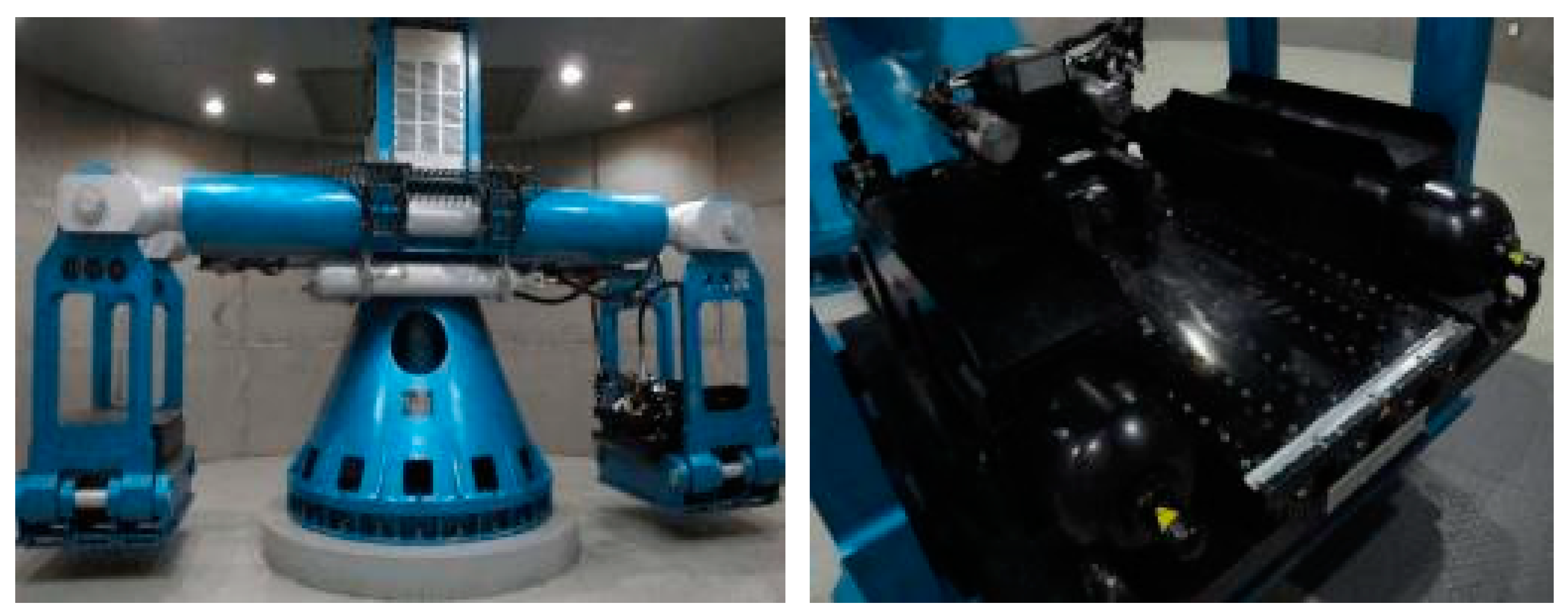
2.3.1. DMA Test

To study the dynamic viscoelastic constitutive model of polymer materials, the DMA tests [40] were carried out. In these tests, parameters of the material’s dynamic viscoelasticity, storage modulus, and loss factor were tested. Then the dynamic viscoelastic constitutive model of polymer materials was established according to the relationship between parameters and frequency.

2.3.2. Derivation of Model

The generalized Maxwell model, also known as the spring-dashpot combination model, consists of multiple Maxwell units connected in parallel. Each Maxwell unit includes an elastic strain spring with an elastic modulus of $E_i$ and a viscous strain dashpot with a corresponding viscosity of ${\eta }_i$ as shown in Figure 4. This model accurately describes the stress relaxation behavior and viscoelastic properties of viscoelastic materials under dynamic loads. It is composed of multiple elements, corresponding to the complex relaxation times of high-polymer grouting materials due to their complex composition. The parameters of the model are relatively easy to obtain and can be acquired through fitting DMA test data to calculate the viscoelastic constitutive model parameters. The parameters obtained from the generalized Maxwell model can be directly applied in finite element software for efficient dynamic response analysis of materials. Thus, this model finds wide applications. Consequently, in the preliminary research and subsequent finite element analysis, the generalized Maxwell model is adopted as the dynamic viscoelastic constitutive model of polymer materials based on DMA test results. The generalized Maxwell model provides an intuitive reflection of the stress-relaxation behavior of materials.

The storage modulus $E^{\mathrm{’}}$ and loss modulus $E^{″}$ of the generalized Maxwell model are expressed as follows:

$$E^{\prime }=E_e+{\sum }_{i=1}^n{E}_i\frac{{\omega }^2{\tau }_i^2}{1+{\omega }^2{\tau }_i^2}$$

(17)

$$E^{″}={\sum }_{i=1}^n{E}_i\frac{\omega {\tau }_i}{1+{\omega }^2{\tau }_i^2}$$

(18)

In the formula, $E_e$ is the quasi-static modulus, $E_i$ is the elastic modulus of each Maxwell model, and ${\tau }_i$ is the relaxation time. The relationship between relaxation time ${\tau }_i$ and viscosity ${\eta }_i$ is ${\tau }_i={\eta }_i/E_i$.

The expression of the stress relaxation modulus and the physical explanation for the viscoelastic behavior are provided by the Maxwell model. The number of Maxwell units and the relaxation time required vary for different viscoelastic materials. For materials with simple viscoelastic properties, a two- or three-unit Maxwell model can be used. However, more Maxwell units are required for complex models. Additionally, there is uncertainty in selecting the parameters due to the principle of equivalent combinations of different parameter sets. The high computational efficiency of the fourth-order generalized Maxwell model has been verified [41,42] so it was chosen for analysis. The energy storage modulus E′ and loss modulus E$″$ in the fourth-order generalized Maxwell model are as follows:

$$E^{\prime }=E_e+E_1\frac{{\omega }^2{\tau }_1^2}{1+{\omega }^2{\tau }_1^2}+E_2\frac{{\omega }^2{\tau }_2^2}{1+{\omega }^2{\tau }_2^2}+E_3\frac{{\omega }^2{\tau }_3^2}{1+{\omega }^2{\tau }_3^2}+E_4\frac{{\omega }^2{\tau }_4^2}{1+{\omega }^2{\tau }_4^2}$$

(19)

$$E^{″}=E_1\frac{\omega {\tau }_1}{1+{\omega }^2{\tau }_1^2}+E_2\frac{\omega {\tau }_2}{1+{\omega }^2{\tau }_2^2}+E_3\frac{\omega {\tau }_3}{1+{\omega }^2{\tau }_3^2}+E_4\frac{\omega {\tau }_4}{1+{\omega }^2{\tau }_4^2}$$

(20)

In analysis, the lsqcurvefit function program is written by Matlab R2019b software for fitting procedures. The relaxation time is bounded as follows for calculation efficiency:

$${\tau }_1>{\tau }_2>\dots >{\tau }_n$$

(21)

The elastic modulus of Maxwell model is also constrained as follows:

$$0<E_i<E_e,\sum E_i<E_e$$

(22)

Three polymer densities were calculated in the numerical analysis. Take 260 kg/m³, for example. The fourth-orderfourth-order parameters of the dynamic viscoelastic constitutive model are shown in

Table 2. Parameters of the polymer constitutive model (ρ = 260 kg/m³).

Parameter	1	2	3	4
${\tau }_i\left(\mathrm{s}\right)$	1.217	0.212	0.198	0.047
$E_i\left(\mathrm{M}\mathrm{P}\mathrm{a}\right)$	4.273	0.077	0.179	1.009

.

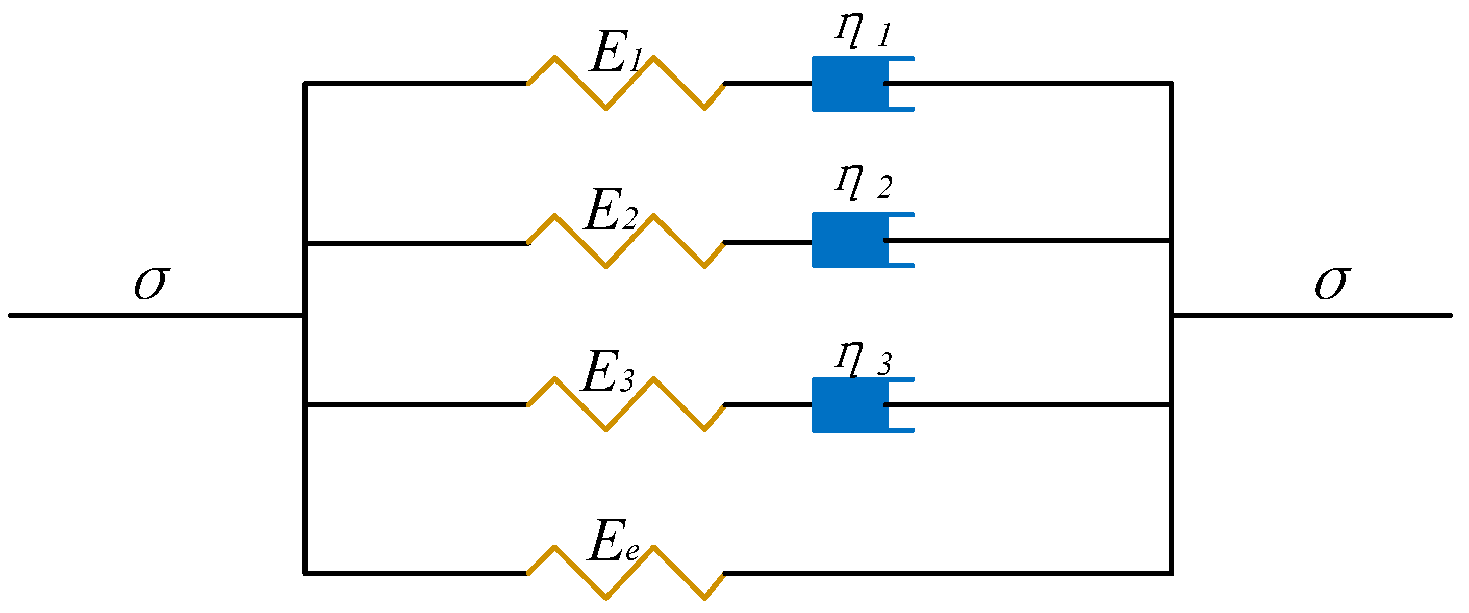
2.3.3. Development of Generalized Maxwell Model

(1)

Differential derivation of generalized Maxwell model

In this paper, a fourth-order generalized Maxwell model is derived to determine the stress increment at the current time step. The finite difference scheme of the Maxwell model is:

$$\frac{\mathsf{\Delta }{u}_1}{\mathsf{\Delta }t}=\frac{F_1^{n+1}-F_1^n}{k_1\mathsf{\Delta }t}+\frac{F_1^{n+1}+F_1^n}{2{\eta }_1}$$

(23)

In the formula, ${\dot{u}}_1$ is the velocity, $F_1$ is the force, $k_1$ is the elastic modulus, and ${\eta }_1$ is the viscosity coefficient. Simplifying the formula as follows:

$$F_1^{n+1}=\frac{1}{1+\frac{k_1\mathsf{\Delta }t}{2{\eta }_1}}\left(F_1^n\left(1-\frac{k_1\mathsf{\Delta }t}{2{\eta }_1}\right)+k_1\mathsf{\Delta }u\right)$$

(24)

In the formula, $F_1^n$ is the force of the previous step and $F_1^{n+1}$ is the force of the current step.

Equating the above equation to the stress-strain relationship, the expression is listed as follows:

$${\sigma }_{1d\_ij}^{n+1}=\frac{1}{1+\frac{G_1\mathsf{\Delta }t}{2{\eta }_1}}\left({\sigma }_{1d\_ij}^n\left(1-\frac{G_1\mathsf{\Delta }t}{2{\eta }_1}\right)+G_{1}2\mathsf{\Delta }{\epsilon }_{ij}^d\right)$$

(25)

In the formula, ${\sigma }_{1d\_ij}^{n+1}$ is the bias stress of the current step, ${\sigma }_{1d\_ij}^n$ is the bias stress of the previous step, $G_1$ is the shear modulus and $\mathsf{\Delta }{\epsilon }_{ij}^d$ is the bias strain increment.

The spherical stress can be expressed as follows:

$${\sigma }_1^{iso}=\frac{1}{3}{\sigma }_1^0+K_1\mathsf{\Delta }{\epsilon }_{kk}$$

(26)

In the formula, $K$ is the bulk modulus.

In the generalized Maxwell model, multiple Maxwell models are in parallel relationships with each other, and a single spring could be viewed as a simplified version of a Maxwell body. Hence, the expression of the total deflection stress of the fourth-order Maxwell is listed as follows:

$$\begin{array}{ll}{\sigma }_{d\_ij}^{n+1}={\sigma }_{1d\_ij}^{n+1}+& {\sigma }_{2d\_ij}^{n+1}+{\sigma }_{3d\_ij}^{n+1}+{\sigma }_{4d\_ij}^{n+1}+{\sigma }_{5d\_ij}^{n+1}\\ & =\frac{1}{1+\frac{G_1\mathsf{\Delta }t}{2{\eta }_1}}\left({\sigma }_{1d_{ij}}^n\left(1-\frac{G_1\mathsf{\Delta }t}{2{\eta }_1}\right)+G_{1}2\mathsf{\Delta }{\epsilon }_{ij}^d\right)\\ & +\frac{1}{1+\frac{G_2\mathsf{\Delta }t}{2{\eta }_2}}\left({\sigma }_{2d_{ij}}^n\left(1-\frac{G_2\mathsf{\Delta }t}{2{\eta }_2}\right)+G_{2}2\mathsf{\Delta }{\epsilon }_{ij}^d\right)+\dots \end{array}$$

(27)

Then the total spherical stress expression of the fourth-order Maxwell model is:

$$\begin{array}{l}{\sigma }^{iso}={\sigma }_1^{iso}+{\sigma }_2^{iso}+{\sigma }_3^{iso}+{\sigma }_4^{iso}+{\sigma }_4^{iso}=\frac{1}{3}{\sigma }_{1\_kk}^0+K_1\mathsf{\Delta }{\epsilon }_{kk}\\ +\frac{1}{3}{\sigma }_{2\_kk}^0+K_2\mathsf{\Delta }{\epsilon }_{kk}+\frac{1}{3}{\sigma }_{3\_kk}^0+K_3\mathsf{\Delta }{\epsilon }_{kk}+\dots \end{array}$$

(28)

(2)

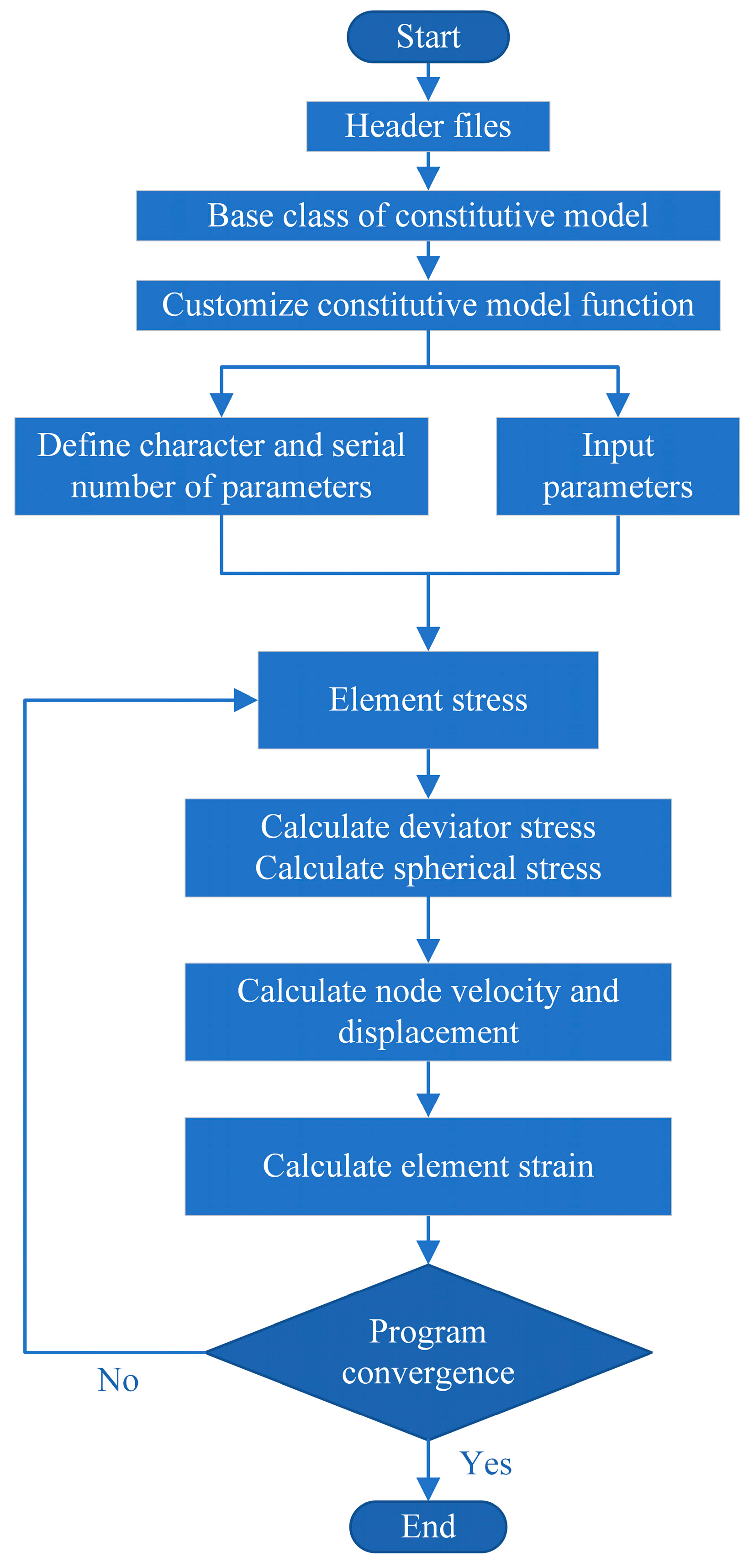
Program development

The fourth-order generalized Maxwell model is developed in VC++. Development work includes modifying header files (.H) and source files (.CPP) and generating dynamic link library files (.DLL) for the main program to call.

The program flow chart of the generalized Maxwell model is shown in Figure 5.

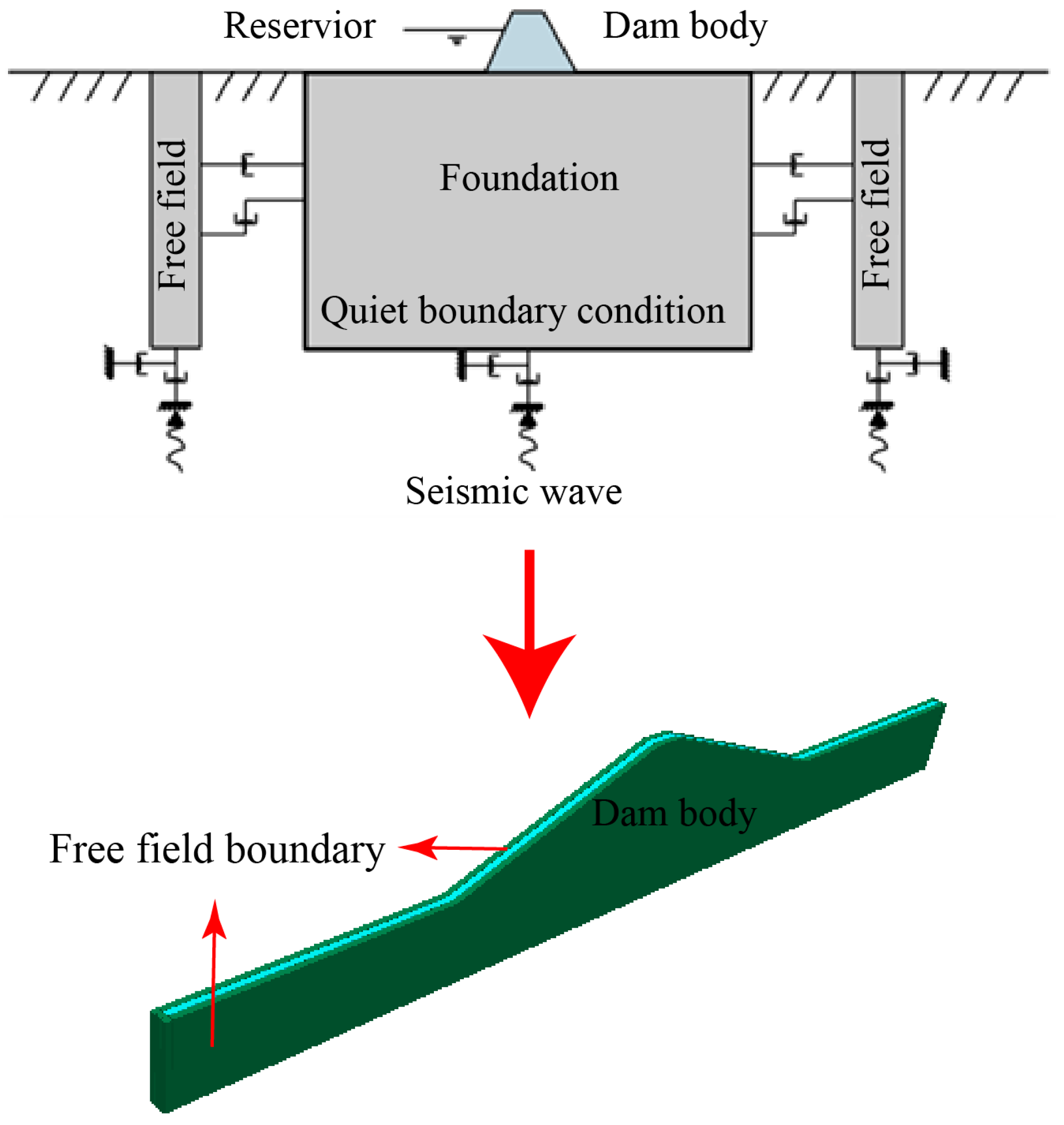
2.4. Dynamic Fluid-Solid Coupling Model

The dynamic fluid-solid coupling model of an earth-rock dam with a polymer antiseepage wall was established by applying the free-field boundary, adding mechanical damping, and using the dynamic viscoelastic constitutive model of polymer materials.

2.4.1. Boundary Conditions

In dynamic calculation, the free-field boundary condition is set to eliminate the wave-reflecting effect, as shown in Figure 6, which is from the dynamic analysis manual of FLAC (Itasca). If body grids and free-field grids move in the same manner, the normal dampers are not activated; if not, the dampers take a static boundary approach to absorb the seismic energy. The body grids were assumed to be uniform.

2.4.2. Earthquake Wave

The El−Centro wave, the first seismic wave captured by humans, has been widely used in model tests and numerical analyses. To accurately recreate the original earthquake waveform, the El Centro wave with an acceleration amplitude of 0.4 g was selected. The acceleration time curve is shown in Figure 7.

To study the impact of different seismic wave acceleration amplitudes on the model, seismic waves with acceleration amplitudes of 0.05, 0.1, 0.2, and 0.4 g were simulated in this experiment. These seismic waves correspond to seismic intensities of VI, VII, VIII, and IX degrees, respectively. In this experiment, El-Centro waves with different peak values will be applied to the bottom of the model, ranging from smallest to largest and lasting for 20 s, as working conditions 1 to 4.

2.4.3. Damping

Internal material friction and potential slippage of the contact surface cause damping. Rayleigh damping has been often used in the structures and dynamic analysis of elastomers to reduce the self-oscillation amplitude of the mode.

Assuming that the damping matrix C is related to the stiffness matrix K and the mass matrix M:

$$C=\alpha M+\beta K$$

(29)

In the formula, the damping constants $\alpha$ and $\beta$ are proportional to mass and stiffness, respectively, determined by the following equation:

$$\alpha ={\zeta }_{min}{\omega }_{min}$$

(30)

$$\beta ={\zeta }_{min}/{\omega }_{min}$$

(31)

In the formula, ${\zeta }_{min}$ is the critical damping ratio, and generally set to 0.05 [43] in the calculation of geotechnical materials, and ${\omega }_{min}$ is the minimum center frequency.

3. Results and Discussion

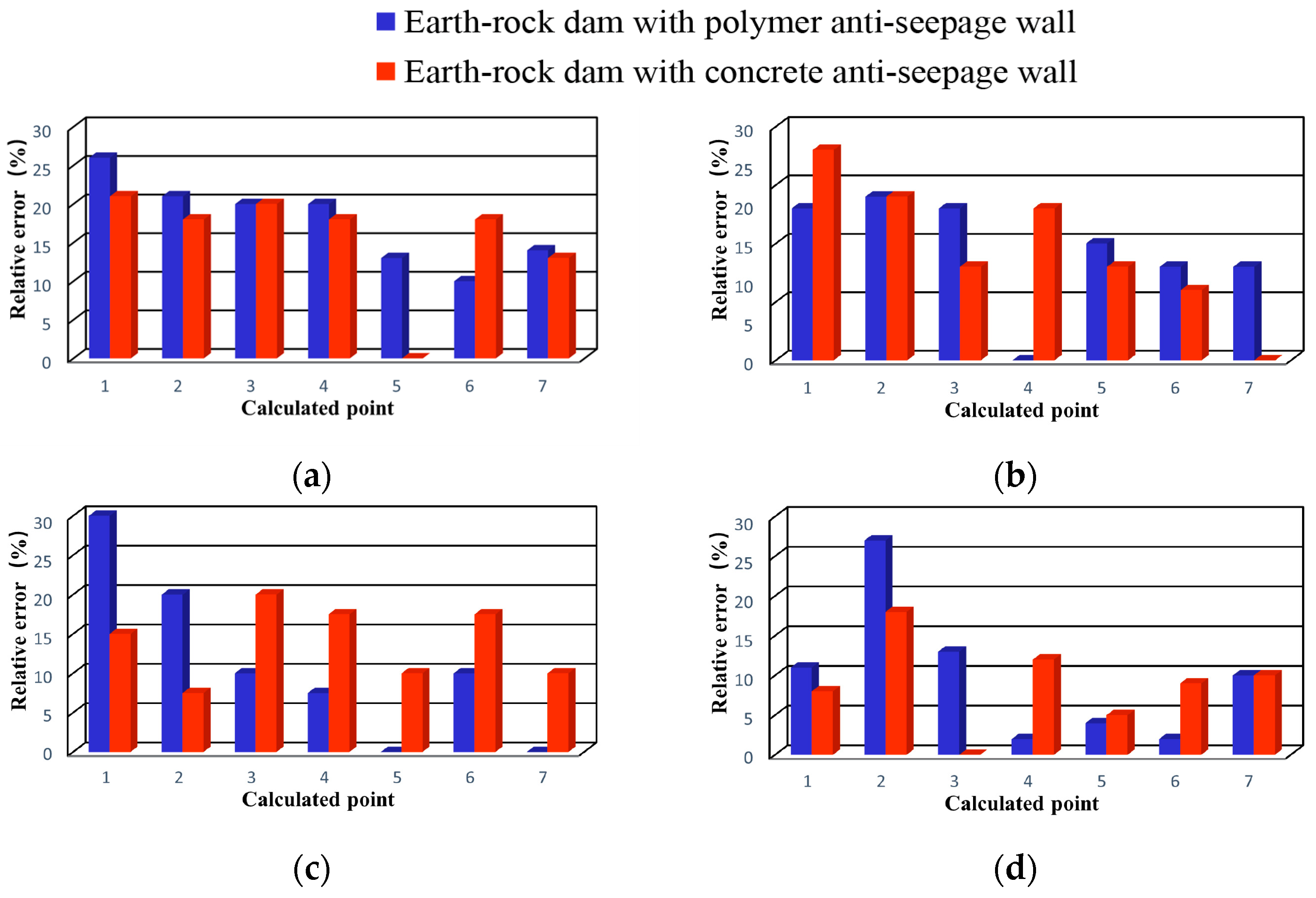
3.1. Model Verification

The centrifuge vibration table increases the gravity on the model by high-speed rotation, enabling the model to reach the stress state of the prototype and replicate the structural characteristics in the model, facilitating the observation of possible deformations and damages to the structure. To study the seismic response of earth-rock dams with polymer antiseepage walls and concrete antiseepage walls, centrifuge tests were carried out in the National Key Laboratory of Soft Soils and Geoenvironmental Engineering (Zhejiang University). The ZJU400 geotechnical centrifuge and vibration table for tests are shown in Figure 8.

The similar relationship between the non-uniform stress centrifuge model and the prototype can be determined based on the similarity of the stress-strain relationship, as depicted in

Table 3. Similarity relation of earth-rock dams.

Physical Quantity	Dimension	Similarity Relation	Similarity Ratio
Length, l	$\left[L\right]$	$C_l$	$1\times {10}^{-2}$
Density, $\rho$	[$\rho$]	$C_{\rho }$	1
Elastic modulus, E	[$E$]	$C_E$	1
Gravity, g	[$a$]	$C_g$	50
Area, s	${\left[L\right]}^2$	$C_s=C_l^2$	$1\times {10}^{-4}$
Mass, m	[$\rho$][$L$]3	$C_m=C_{\rho }{C}_l^3$	$1\times {10}^{-6}$
Force, F	[$\rho$][$L$]3[$a$]	$C_F$ =$C_{\rho }{C}_l^3{C}_a$	$7.07\times {10}^{-5}$
Load, P	[$\rho$][$L$]2[$a$]	$C_P$= $C_{\rho }{C}_l^2{C}_a$	$7.07\times {10}^{-3}$
Vibration frequency, f	[$L$]−1/2[$a$]1/2	$C_f$ = ${(C_a/C_l)}^{1/2}$	84.08
Speed, v	[$L$]1/2[$a$]1/2	$C_v$ =${\left(C_a{C}_l\right)}^{1/2}$	0.84
Acceleration, EI	[$a$]	$C_A$ =$C_a$	70.7
Stress, σ	[$\rho$][$L$][$a$]	$C_{\sigma }$ = $C_{\rho }{C}_l{C}_a$	0.71
Strain, ε	[$\rho$][$L$][$a$]/[$E$]	$C_{\epsilon }$=$C_{\rho }{C}_l{C}_a/C_E$	0.71

. The geometric similarity ratio of the dynamic centrifuge test is 1/100, while the acceleration similarity ratio for the centrifuge rotation is 50 g, based on the size of the prototype and the centrifuge test model box. In terms of the dam design parameters, the dam has a height of 15 cm, a foundation thickness of 15 cm, a top width of 5 cm, and a bottom width of 73 cm. The ratio of the upstream and downstream dam slopes is 1:2.3. Moreover, the antiseepage wall has a height of 17 cm and extends 2 cm into the dam foundation.

The dynamic fluid-solid coupling calculation was performed for working conditions 1–4. The model extracted the peak acceleration at the monitoring points corresponding to the experimental measurements to determine the simulated and experimental peak acceleration values of the impermeable wall in the earth-rock dam. The difference between these values represented the relative error, which was visualized in Figure 9. Additionally, the average relative error and variance are presented in

Table 4. Acceleration response error under different conditions.

	Average Value/%	Variance/%
Earth-rock dam model with	10.4	7.4
polymer antiseepage wall	9.9	6.3

.

From the analysis, the average relative error between the calculated results and the centrifuge test results is 10.4% and 9.9%, with the variance being 7.4% and 6.3%, respectively. The calculated peak acceleration values at each measurement point were close to the experimental values. The finite element numerical model of the earth-rock dam with a polymer antiseepage wall effectively reflects the acceleration response of the earth-rock dam under seismic action. Therefore, it is considered that the finite element numerical model is reasonable. So the dynamic simulation model was used for the following analysis.

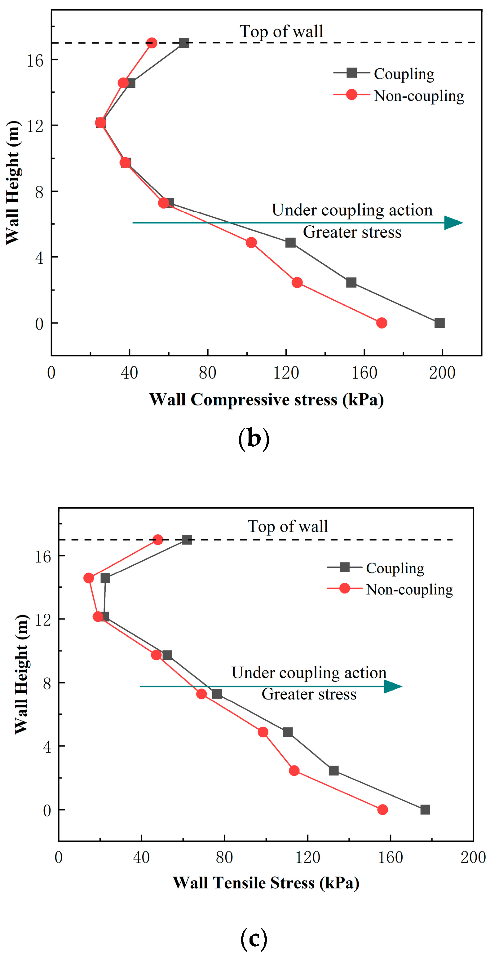
3.2. Coupling Effect

Seismic response analysis is conducted under working condition 4 to study the effects of fluid-solid coupling of an earth-rock dam with a polymer antiseepage wall. According to Figure 10, the peak acceleration of the antiseepage wall increases progressively along its height, with the maximum acceleration observed at the top. Under the influence of the coupling effect, the peak acceleration of the wall exceeds that under non-coupling conditions. This is because, after considering the fluid-structure interaction, the upstream reservoir water has simultaneous effects on both the stress field and the seepage field of the earth-rock dam, resulting in an increased acceleration response. During an earthquake, the earth-rock dam constrains the movement of the polymer antiseepage wall. Therefore, the peak acceleration of the wall is significantly higher under the coupling effect. The compressive stress of the antiseepage wall initially decreases along the wall height and then increases, with the maximum compressive stress located at the bottom of the wall. Under coupling and non-coupling conditions, the maximum values are 202 kPa and 162 kPa, respectively, and the magnitude of the amplification is 25%. Similarly, the tensile stress initially increases along the wall height and then decreases, with the maximum tensile stress located at the bottom of the wall. Under coupling and non-coupling conditions, the maximum tensile stress values are 177 kPa and 156 kPa, respectively, showing a 13% increase in the maximum tensile stress when considering coupling effects.

The displacement distribution pattern of the polymer antiseepage wall, as depicted in Figure 11, demonstrates the following characteristics: The displacement decreases with increasing wall height, with the maximum displacement occurring at the top of the wall. Specifically, under coupling and non-coupling conditions, the maximum displacements of the antiseepage wall are 9.94 cm and 2.99 cm, respectively. The coupling effect significantly affects the displacement of the antiseepage wall. This can be attributed to the coupling effect, which causes an increased displacement of the earth-rock dam due to the influence of the seepage field. Due to the constraint imposed by the earth-rock dam, the displacement of the polymer antiseepage wall also increases.

In conclusion, coupling effects should not be ignored in the safety evaluation and analysis of earth-rock dams [44]. After considering these effects, it is found that the acceleration, stress, and displacement of the polymer antiseepage wall are relatively larger than before. Therefore, in the subsequent calculations, the fluid-solid coupling effects between the soil skeleton and pore water will be taken into account.

3.3. Influence Factors

3.3.1. Reservoir Water Level

The variation in reservoir water level not only affects the stress fields and seepage fields of the earth-rock dam but also influences the acceleration, stress, and deformation behavior of the dam under seismic response. In this study, the effect of water level on earth-rock dams with polymer antiseepage walls was investigated at four different levels: 1 m, 5 m, 9 m, and 13 m, aiming to simulate the different conditions during low and high water periods.

The peak acceleration of the polymer antiseepage wall at different reservoir water levels is shown in Figure 12a. It shows that when the water level is the same, the acceleration increases with wall height, and the greatest acceleration occurs at the top of the wall. For example, the acceleration at the top of the wall is 0.70 g, 0.72 g, 0.74 g, and 0.75 g, respectively, with the water level being 1 m, 5 m, 9 m, and 13 m. From Figure 12b,c, the compressive and tensile stresses first decrease then increase from the bottom to the top of the wall. The greatest compressive and tensile stresses occur at the bottom of the wall. The great compressive stress is 165 kPa, 175 kPa, 201 kPa, and 231 kPa, respectively, and the great tensile stress is 145 kPa, 159 kPa, 180 kPa, and 206 kPa, respectively, at the water levels of 1 m, 5 m, 9 m, and 13 m. From Figure 12, it can be observed that the peak acceleration, compressive, and tensile stresses of the dam increase with the water level. This is due to the fact that the dam experiences greater pressure when the water level is higher. As the water level of the dam increases, it experiences less effective stress in horizontal and vertical directions, thus leading to its loss of stability.

Figure 13 shows that the displacement increases from the bottom to the top of the wall, and the greatest displacement occurs at the top of the wall, with values of 3.68 cm, 7.84 cm, and 10.06 cm, respectively, at water levels of 1 m, 5 m, 9 m, and 13 m. However, when the water level is 13 m, the displacement first increases then decreases from the bottom to the top of the wall, with a maximum displacement of 12.57 cm at the middle of the wall. According to the lateral comparison, the rising water level may result in the horizontal and vertical permanent displacement of the dam and the displacement of the antiseepage wall.

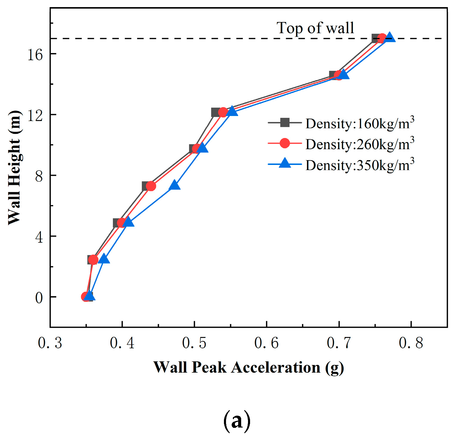
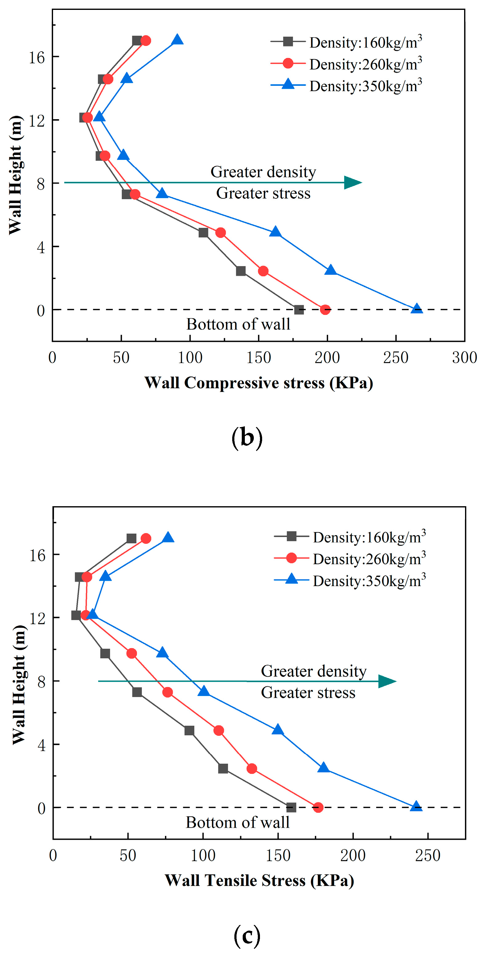
3.3.2. Wall’s Density

The mechanical properties of polymer materials, including their density, play a significant role [22]. This section analyzed the seismic response of the earth-rock dam with a polymer antiseepage wall at three different densities: 160 kg/m³, 260 kg/m³, and 350 kg/m³. This analysis takes into account the impact of density on construction costs. The input peak seismic acceleration was 0.4 g, and the water level was 8.6 m.

The peak acceleration of the polymer antiseepage wall increases slightly with density, as shown in Figure 14a. From Figure 14b, the compressive stress first decreases then increases from the bottom to the top of the wall, and the greatest compressive stress occurs at the bottom of the wall with values of 179 kPa, 199 kPa, and 265 kPa, respectively. From Figure 14c, the tensile stress has the same law as the compressive stress. The displacement of the polymer antiseepage wall is shown in Figure 15. The distribution increases from the bottom to the top of the wall, and the greatest displacement occurs at the top of the wall with values of 10.04 cm, 9.94 cm, and 9.71 cm, respectively.

This section shows that the distribution of the acceleration, stress, and displacement of the antiseepage wall at different densities is very similar. The acceleration increases with the density, while the difference is small as the wall shares little energy during seismic response due to the polymer antiseepage wall’s small volume and mass compared with the dam. The compressive and tensile stresses of the wall increase with density; this may be due to the elastic modulus of the polymer material increasing, as structures with higher stiffness experience a larger seismic response than structures with lower stiffness.

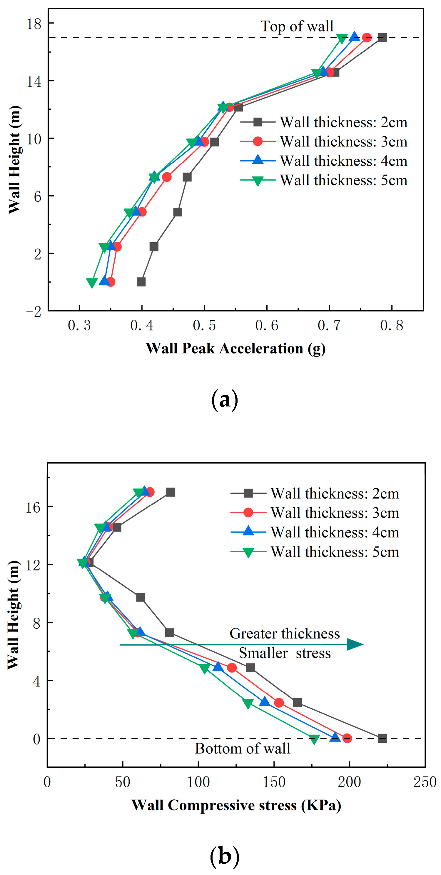
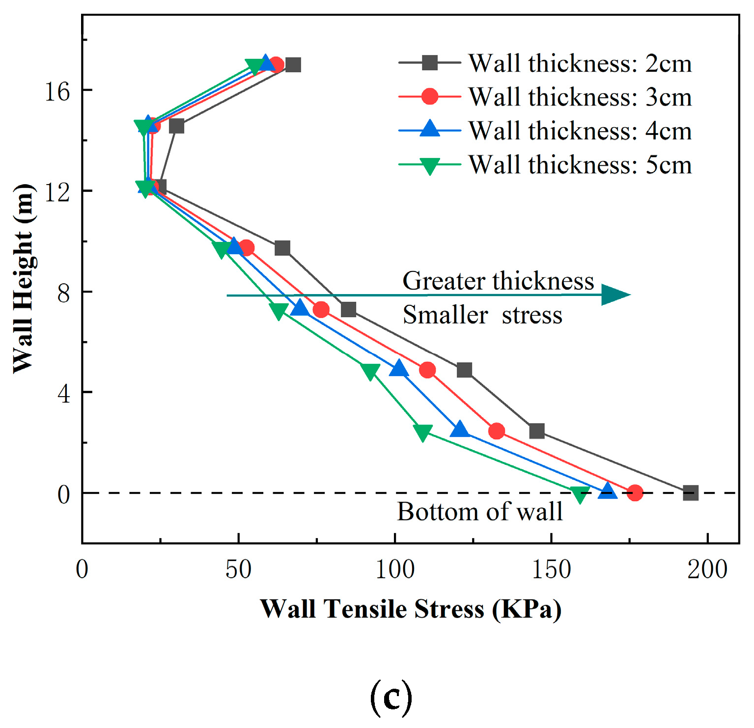
3.3.3. Wall’s Thickness

To satisfy the needs of seepage control and reinforcement in dam projects, various thicknesses of antiseepage walls can be formed using polymer grouting based on the width of the slot. In this study, wall thicknesses of 2 cm, 3 cm, 4 cm, and 5 cm were used to analyze the seismic response of earth-rock dams with polymer antiseepage walls under the fluid-solid coupling effect.

From Figure 16a, the acceleration increases from the bottom to the top of the wall, and the greatest acceleration occurs at the top of the wall. From Figure 16b,c, the compressive stress first decreases then increases with the increase in wall thickness. The greatest compressive stress occurs at the bottom of the wall; for example, the greatest compressive stress of the wall is 222 kPa, 199 kPa, 190 kPa, and 177 kPa, respectively, and the greatest tensile stress is 195 kPa, 177 kPa, 168 kPa, and 159 kPa, respectively. Figure 17 shows the displacement of polymer antiseepage walls with different wall thicknesses. The distribution of the displacement increases from the bottom to the top of the wall, and the greatest distribution occurs at the top of the wall. When the thickness is 2 cm, 4 cm, or 5 cm, the greatest displacement of the wall is 10.56 cm, 9.92 cm, and 9.87 cm, respectively.

These figures show that as the wall’s thickness increases, the acceleration, compressive, and tensile stresses all decrease. This phenomenon may be attributed to the increased energy dissipation of the wall. Further, because the movement of the antiseepage wall is constrained by the dam during seismic response, the acceleration of the wall differs by a relatively small amount at different thicknesses.

3.3.4. Wall’s Materials

In order to compare the differences between the dam with the polymer wall and the dam with the traditional concrete wall, dynamic fluid-solid coupling calculations were performed on earth-rock dams with polymer and concrete antiseepage walls under working conditions 1–4. The results are shown in Figure 18. The development tendency of acceleration increases with the wall height and the input seismic acceleration, and the greatest acceleration occurs at the top of the wall. The peak accelerations of polymer and concrete antiseepage walls are shown in

Table 5. Peak accelerations of antiseepage walls.

Working Condition	Polymer Wall (g)	Concrete Wall (g)
1	0.12	0.13
2	0.20	0.23
3	0.39	0.43
4	0.76	0.81

. The trends of peak acceleration for the two types of antiseepage walls are generally in agreement. A polymer antiseepage wall’s peak acceleration is lower than that of a concrete one under the same working conditions; this is because polymer materials have a lower stiffness and lighter mass than concrete materials.

The greatest compressive and tensile stresses of the two types of antiseepage walls under working conditions 1–4 are shown in Figure 19 and Figure 20. It can be seen that under seismic response, the polymer wall’s greatest compressive and tensile stresses both occur at the bottom of the wall. The greatest compressive stress of the wall under is 138 kPa, 154 kPa, 175 kPa, and 199 kPa, respectively, and the value of the greatest tensile stress is 126 kPa, 139 kPa, 154 kPa, and 177 kPa, respectively. By comparison, the maximum compressive stress of the concrete wall occurs at the bottom of the wall, while the maximum tensile stress of the concrete wall is near the bottom. The greatest compressive stresses of the concrete wall are 645 kPa, 821 kPa, 1443 kPa, and 2561 kPa, respectively. The maximum tensile stress of the wall is 1004 kPa, 1069 kPa, 1242 kPa, and 1686 kPa, respectively. It is seen from these figures that the polymer antiseepage wall experiences smaller maximum compressive and tensile stresses than the concrete wall because the modulus of elasticity of polymer materials is similar to the adjacent soil, and polymer materials have elastomeric characteristics that provide some flexibility under seismic response.

The relationship between the compressive and tensile strengths of polymer materials at various densities is depicted in Figure 21. As indicated in the figure, the compressive and tensile strengths of polymer materials with a density of 260 kg/m³ are 4540 kPa and 3350 kPa, respectively, and the maximum compressive and tensile stress experienced by the polymer antiseepage wall during an earthquake are lower than their strengths. This yields sufficient safety reserves. In comparison, the compressive and tensile strengths of the concrete material are usually 25,000 kPa and 1500 kPa, respectively. However, under working condition 4, the maximum tensile stress of the concrete antiseepage wall has exceeded its tensile strength, leading to tensile damage. The concrete damage can be predicted from Figure 20b; it can also be proved by the results of the centrifuge test shown in Figure 22.

The excavation result of the dynamic centrifuge test is shown in Figure 22. The polymer wall appears to be in good overall condition. In contrast, the concrete wall has cracks near the bottom, resulting in failure on both sides of the wall, which impacts the impermeability of the earth-rock dam. The test results are in accordance with the results of the numerical simulation, which indicates that the established numerical model is a reasonable model.

4. Conclusions

In this study, a dynamic microscopic fluid-solid coupling model was formulated to analyze the behavior of an earth-rock dam with a polymer antiseepage wall. The seismic response of the polymer antiseepage wall was examined, and the seismic stability of the wall was evaluated. The conclusions of this study are as follows:

(1)

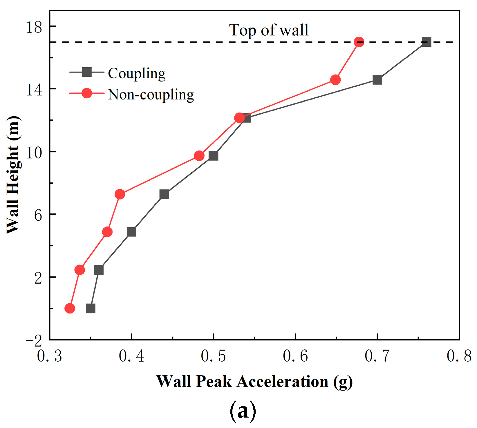
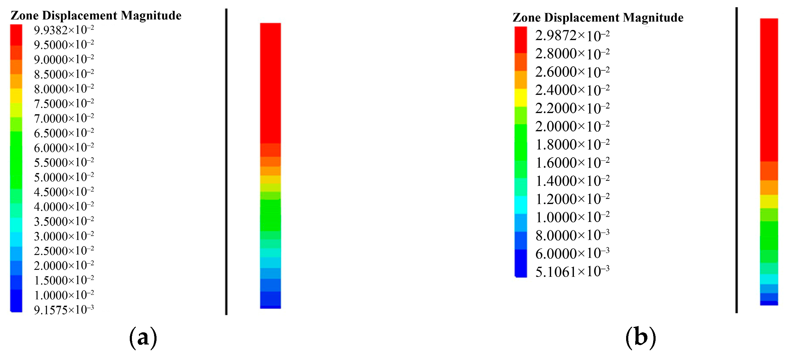
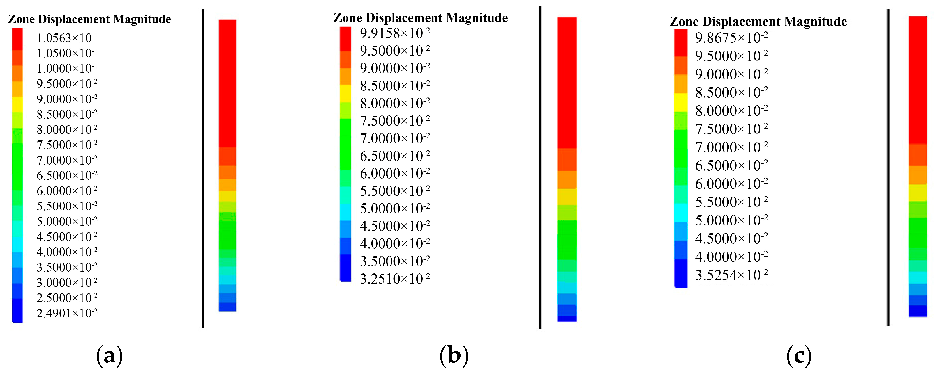
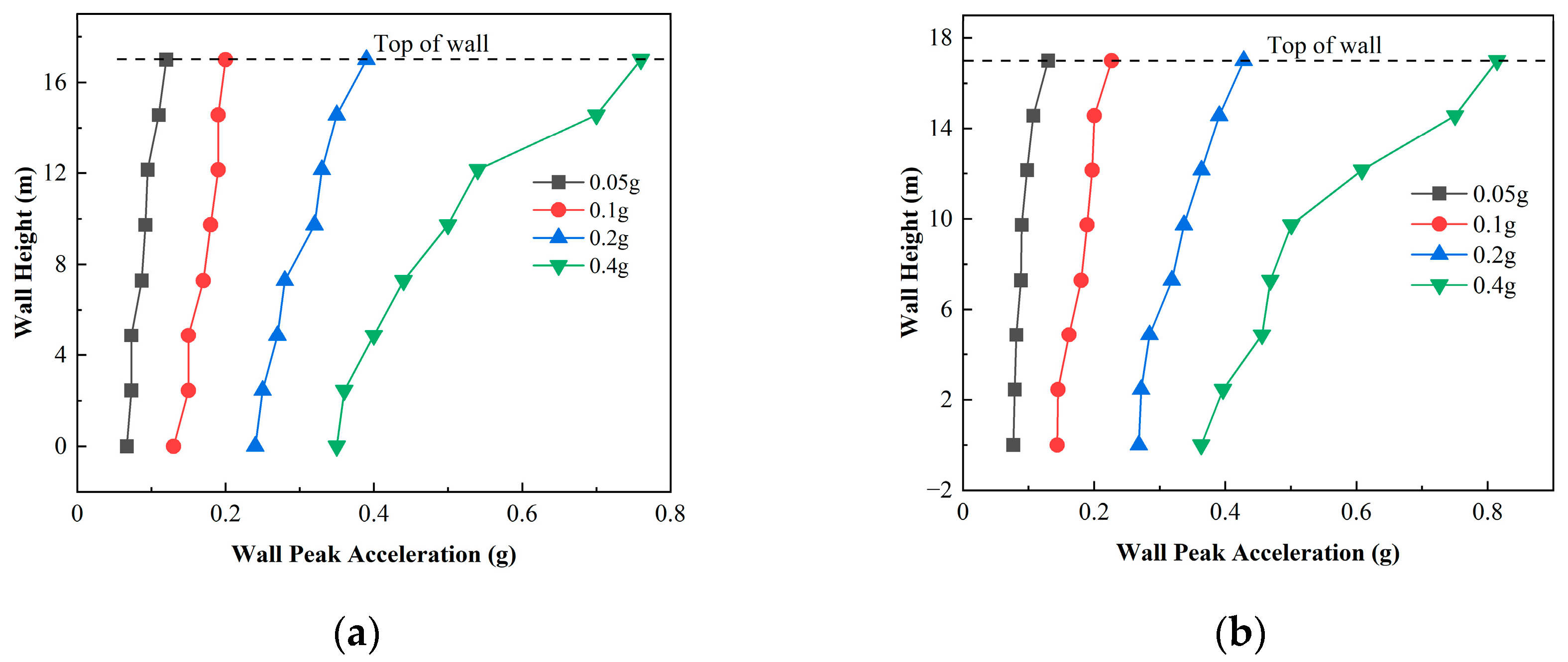
The peak acceleration of the antiseepage wall was observed to increase as a result of the concurrent actions of reservoir water on both the stress field and seepage field of the earth-rock dam. This increase in the dam’s acceleration response consequently led to an elevation in the peak acceleration of the wall. Additionally, the application of microscopic fluid-solid coupling had a notable impact, resulting in a 25% and 13% increase, respectively, in both the maximum compressive and tensile stresses experienced by the wall. Moreover, the displacement of the polymer antiseepage wall experienced a significant increase due to the constraints imposed by the earth-rock dam. Consequently, it is imperative to consider the effect of fluid-solid coupling in the safety assessment and analysis of earth-rock dams.

(2)

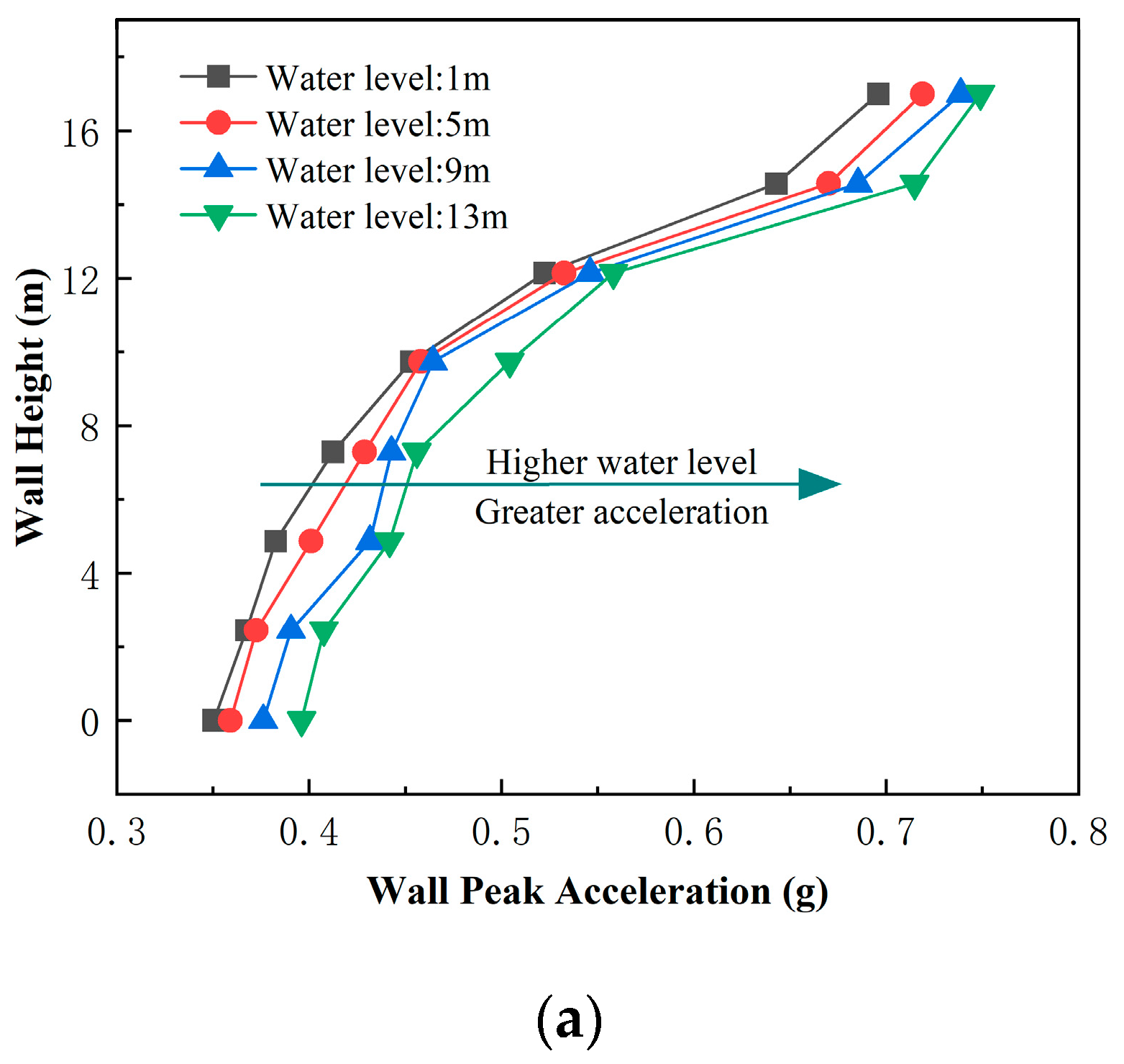
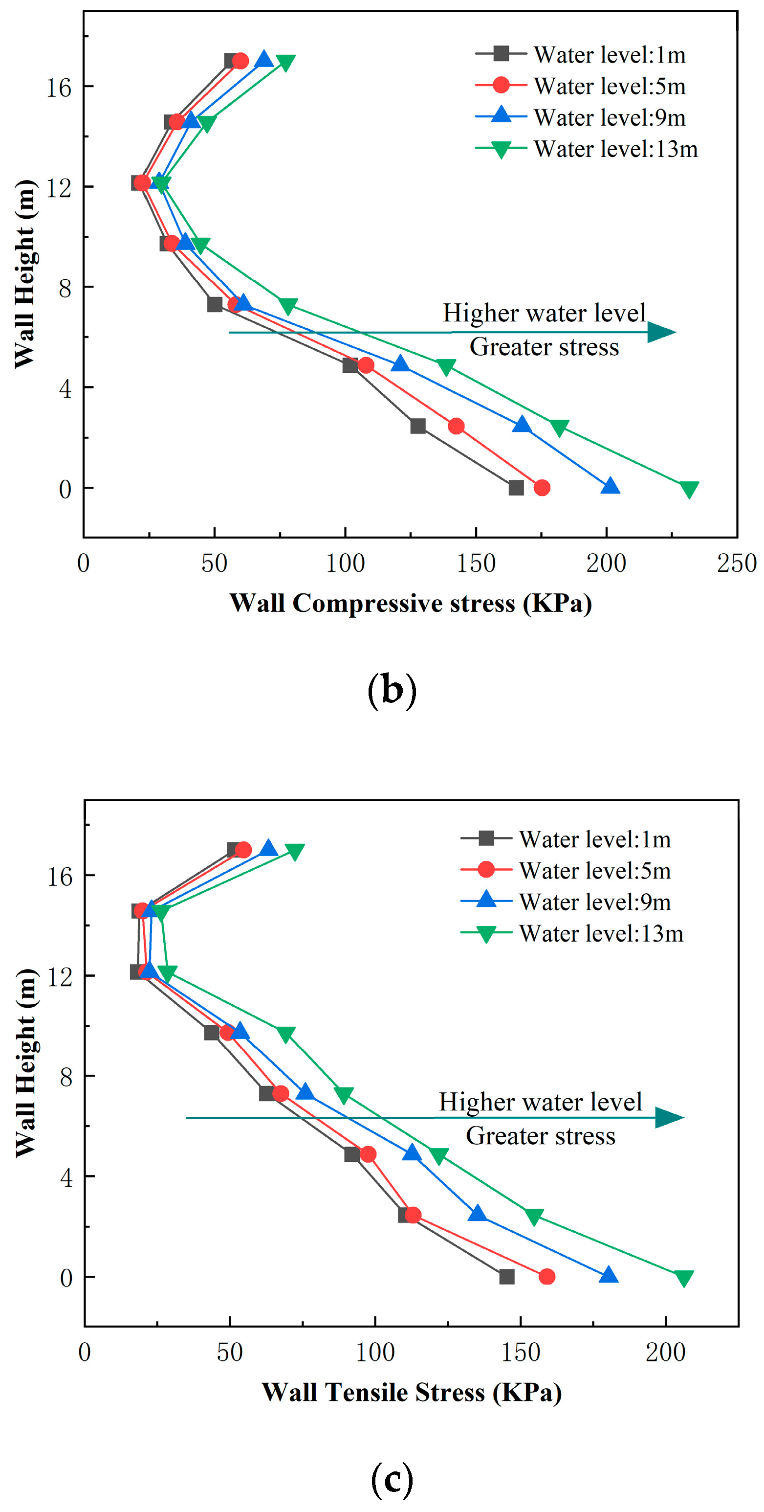
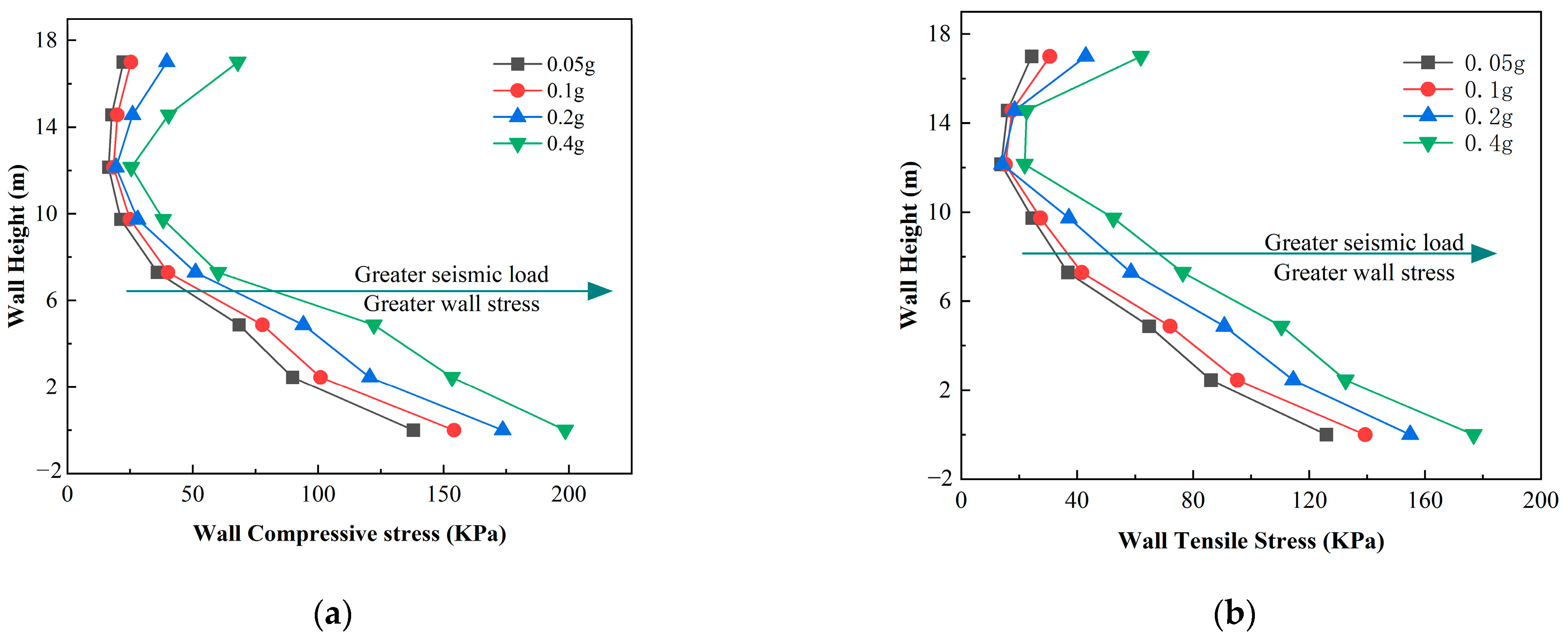
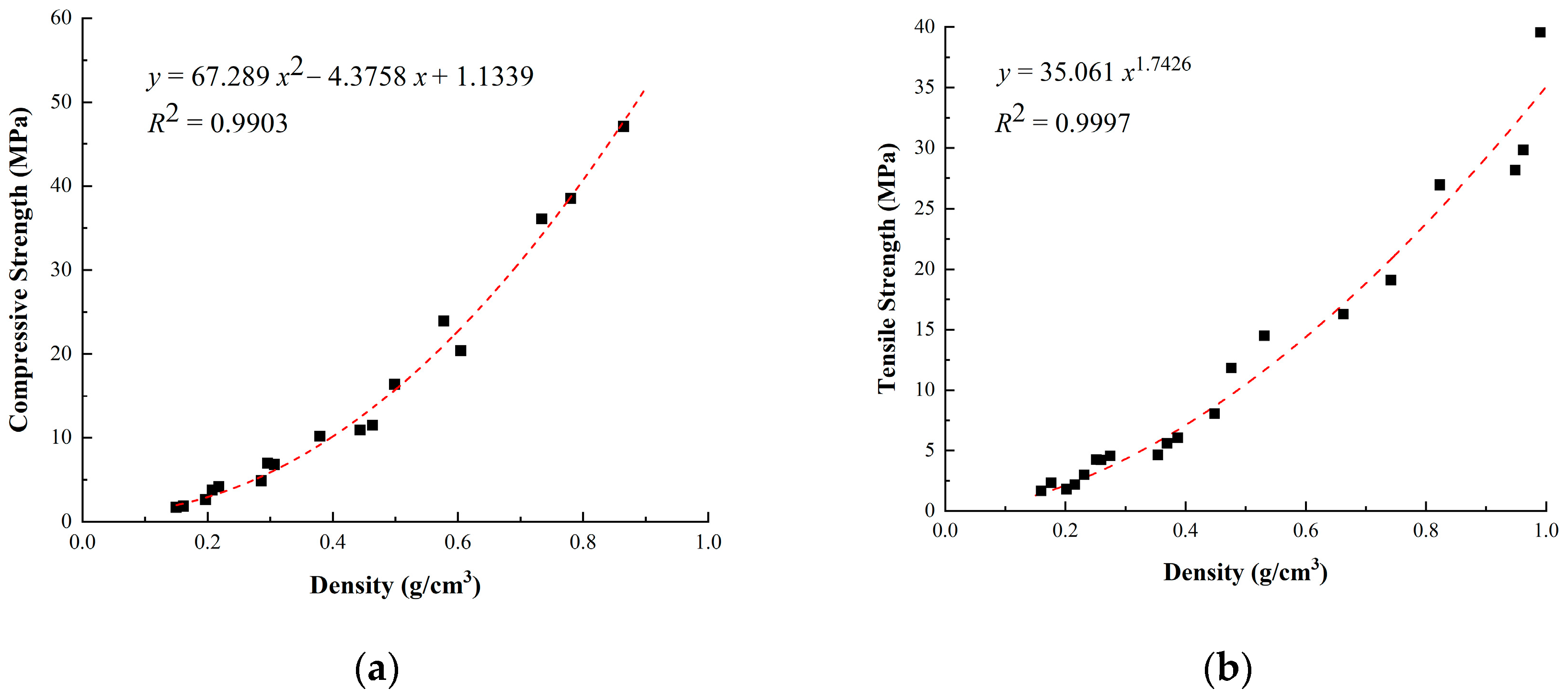
Considering the effect of fluid-solid coupling, the peak acceleration, dynamic stress, and displacement of the polymer antiseepage wall increased progressively as the water level rose. Furthermore, the acceleration, compressive stress, and tensile stress of the polymer antiseepage wall also increased with the density of polymer materials due to the increased stiffness and seismic response of the wall. However, as the wall thickness increased, the acceleration, compressive stress, tensile stress, and displacement of the polymer antiseepage wall decreased due to the enhanced energy dissipation capacity of the wall.

(3)

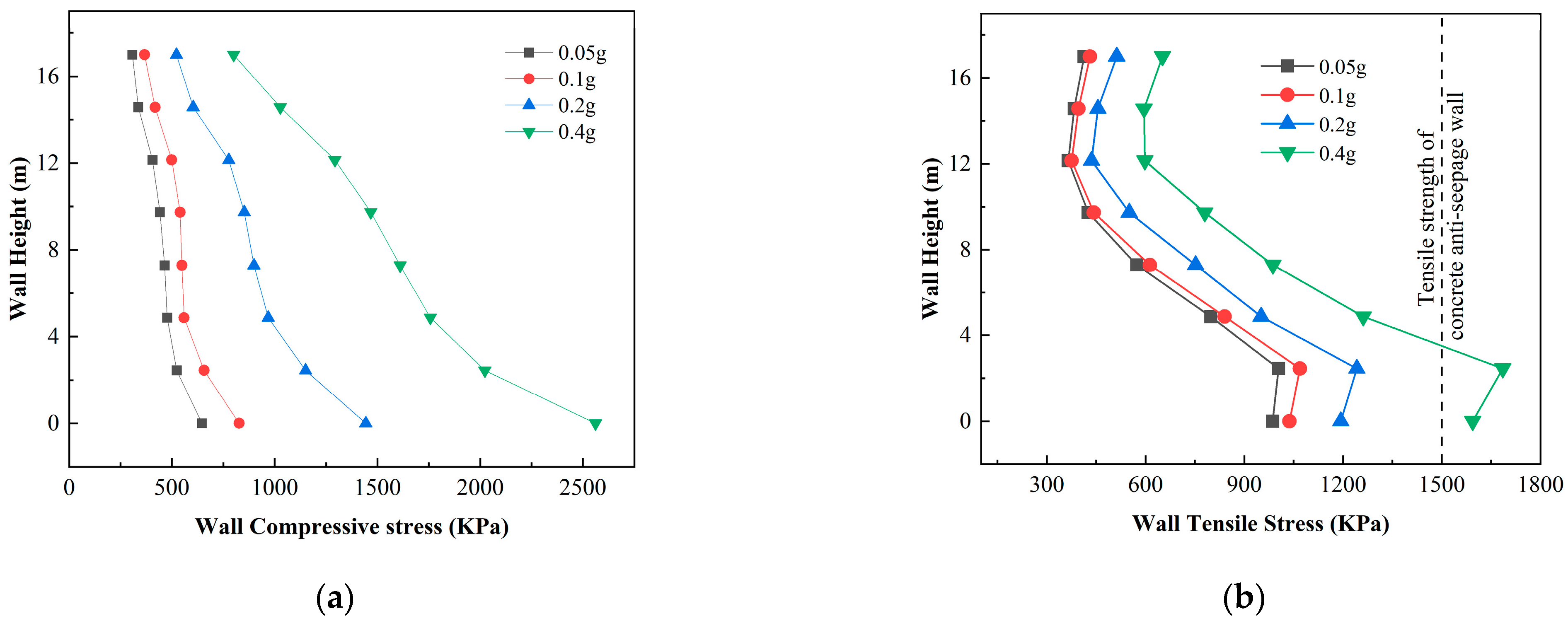
Under the same working conditions, the peak acceleration of the polymer antiseepage wall was smaller than that of the concrete one due to the effect of microscopic fluid-solid coupling. Under the same earthquake, the compressive and tensile stresses of the polymer antiseepage wall were both smaller than their respective compressive and tensile strengths, which indicated sufficient safety reserves. while the tensile stress of the concrete antiseepage wall exceeded its tensile strength, causing the wall to be damaged. The displacement of the polymer antiseepage wall was greater than that of the concrete wall due to the flexible nature of polymer materials and their ability to self-recover from large deformations.

References

- Yang, Q.G.; Tan, J.X.; Zhou, H.Q. Features of High-hazard Potential Dam and Key Issues in Reinforcement Design. China Water Resour. 2008, 20, 34–36. [Google Scholar]
- Wang, F.M.; Li, J.; Shi, M.; Guo, C.C. New Seepage-proof and Reinforcing Technologies for Dikes and Dams and their Applications. J. Hydroelectr. Eng. 2016, 35, 1–11. [Google Scholar]
- Wang, F.M.; Guo, C.C.; Gao, Y. Formation of a Polymer Thin Wall Using the Level Set Method. Int. J. Geomech. 2014, 14, 04014021. [Google Scholar] [CrossRef]
- Guo, C.C.; Chu, X.X.; Wang, F.M. The Feasibility of Non-water Reaction Rolymer Grouting Technology Application in Seepage Prevention for Tailings Reservoirs. Water Sci. Technol.-Water Supply 2018, 18, 203–213. [Google Scholar] [CrossRef]
- Guo, C.C.; Wang, F.M. Mechanism Study on the Construction of Ultra-Thin Antiseepage Wall by Polymer Injection. J. Mater. Civ. Eng. 2012, 24, 1183–1192. [Google Scholar]
- Xu, J.G.; Wang, F.M.; Zhong, Y.H.; Wang, B.; Li, X.L.; Sun, N. Stress Analysis of Polymer Diaphragm Wall for Earth-rock Dams Under Static and Dynamic Loads. Chin. J. Geotech. Eng. 2012, 34, 1699–1704. [Google Scholar]
- Li, J.; Zhang, J.W.; Wang, Y.K.; Wang, B. Seismic Response of Earth Dam with Innovative Polymer Antiseepage Wall. Int. J. Geomech. 2020, 20, 04020079. [Google Scholar] [CrossRef]
- Mao, J.; Chen, X.G.; Wang, Z.H.; Si, M.N. Analysis of Representative Seismic Damage to Reservoirs in the Southeast of Mianyang City during Wenchuan Earthquake. J. Disaster Prev. Mitig. Eng. 2015, 35, 137–144. [Google Scholar]
- Ishihara, K.; Ueno, K.; Yamada, S.; Yasuda, S.; Yoneoka, T. Breach of a tailings dam in the 2011 earthquake in Japan. Soil Dyn. Earthq. Eng. 2015, 68, 3–22. [Google Scholar] [CrossRef]
- Agurto-Detzel, H.; Bianchi, M.; Assumpçao, M.; Schimmel, M.; Collaço, B.; Ciardelli, C.; Barbosa, J.R.; Calhau, J. The tailings dam failure of 5 November 2015 in SE Brazil and its preceding seismic sequence. Geophys. Res. Lett. 2016, 43, 4929–4936. [Google Scholar] [CrossRef]
- Zhao, B.; Wang, Y.S.; Luo, Y.H.; Li, J.; Mang, X.; Shen, T. Landslides and dam damage resulting from the Jiuzhaigou earthquake (8 August 2017), Sichuan, China. Open Sci. 2018, 5, 171418. [Google Scholar] [CrossRef] [PubMed]
- Chen, W.J.; Sun, H.; Chen, Y.N. Recent Advances on Macro-scale and Micro-scale Dynamic Interaction Between High Earth-rock Dams and Water. Adv. Sci. Technol. Water Resour. 2013, 33, 10–16. [Google Scholar]
- Liang, H.A. Research on Earthquake Damage Prediction and Rapid Assessment Methods for Earth and Rock Dams. Recent Dev. World Seismol. 2013, 3, 44–45. [Google Scholar]
- Wang, F.M.; Li, J.M.; Fang, H.Y.; Xue, B.H. Analysis of Polymer Cut-off Walll of Yellow River Dyke. Yellow River 2019, 41, 48–52, 86. [Google Scholar]
- Brynk, T.; Hellmich, C.; Fritsch, A.; Zysset, P.; Eberhardsteiner, J. Experimental Poromechanics of Trabecular Bone Strength: Role of Terzaghi’s Effective Stress and of Tissue Level Stress Fluctuations. J. Biomech. 2011, 44, 501–508. [Google Scholar] [CrossRef] [PubMed]
- Biot, M.A. General Theory of Three-Dimensional Consolidation. Appl. Phys 1941, 12, 155–164. [Google Scholar] [CrossRef]
- Lin, B.H. Research on Theory and Numerical Solution for Inspecting Liquefaction Potentical of a Composite Foundation of Sand-Gravel Columns. Ph.D. Thesis, Xi’an University of Technology, Xi’an, China, 1997. [Google Scholar]
- Jamshid, G.; Edward, L.W. Variational Formulation of Dynamics of Fluid-Saturated Porous Elastic Solids. J. Eng. Mech. 1972, 98, 947–963. [Google Scholar]
- Ghaboussi, J.; Wilson, E.L. Seismic Analysis of Earth Dam-reservoir Systems. ASCE J. Soil Mech. Found Div. 1973, 99, 849–886. [Google Scholar] [CrossRef]
- Zhang, Y.W.; Zhang, X.W.; Wang, Z.; Han, X.K. Stdy on the Seismic Behavior of Earth-Rock Dam Located on the Liquefiable Ground. N. China Earthq. Sci. 2021, 39, 17–22, 65. [Google Scholar]
- Zienkiewicz, O.C.; Chang, C.T.; Bettess, P. Drained, Undrained, Consolidating and Dynamic Behaviour Assumptions in Soils. Géotechnique 1980, 30, 385–395. [Google Scholar] [CrossRef]
- Zienkiewicz, O.C. Basic Formulation of Static and Dynamic Behaviours of Soil and Other Porous Media. Appl. Math. Mech. 1982, 3, 457–468. [Google Scholar] [CrossRef]
- Zienkiewicz, O.C.; Shiomi, T. Dynamic Behaviour of Saturated Porous Media; the Generalized Biot Formulation and its Numerical Solution. Int. J. Numer. Anal. Methods Geomech. 1984, 8, 71–96. [Google Scholar] [CrossRef]
- Pan, Z.Y.; Chen, D.H.; Zhao, Y.Y.; Liu, Y.H. Influence of Foundation and Reservoir Water Models on Seismic Responses of the Gravity Dams. J. China Three Gorges Univ. (Nat. Sci.) 2022, 44, 30–37, 76. [Google Scholar]
- Liu, F.; Wang, Z.Z.; Li, K.Z.; Xu, C.; Wu, F.; Zhang, H.L.; Zhang, X.D. Seismic dynamic responses of spillway radial steel gates considering fluid-solid coupling effects. J. Water Resour. Water Eng. 2021, 32, 158–166. [Google Scholar]
- Wang, C.; Zhang, H.Y.; Zhang, Y.J.; Guo, L.N.; Wang, Y.J.; Htun, T.T.T. Influences on the Seismic Response of a Gravity Dam with Different Foundation and Reservoir Modeling Assumptions. Water 2021, 13, 3072. [Google Scholar] [CrossRef]
- Kong, X.J.; Xing, H.J.; Li, H.J. An Explicit Spectral-Element Approach to Fluid-Solid Coupling Problems in Seismic Wave Propagation. Chin. J. Theor. Appl. Mech. 2022, 54, 2513–2528. [Google Scholar]
- Zhang, M.Z.; Zhang, L.; Wang, X.C.; Su, W.; Qiu, Y.X.; Wang, J.T.; Zhang, C.H. A framework for Seismic Response Analysis of Dams Using Numerical Source-to-structure Simulation. Earthq. Eng. Struct. Dyn. 2023, 52, 593–608. [Google Scholar] [CrossRef]
- Rayegani, A.; Nouri, G. Application of Smart Dampers for Prevention of Seismic Pounding in Isolated Structures Subjected to Near-fault Earthquakes. J. Earthq. Eng. 2022, 26, 4069–4084. [Google Scholar] [CrossRef]
- Rayegani, A.; Nouri, G. Seismic collapse probability and life cycle cost assessment of isolated structures subjected to pounding with smart hybrid isolation system using a modified fuzzy based controller. Structures 2022, 44, 30–41. [Google Scholar] [CrossRef]
- Jing, W.; Wang, J.X. Seismic Dynamic Responses of Earth-Rock Dam Considering Wave and Seepage. J. Vibroeng. 2020, 22, 403–415. [Google Scholar] [CrossRef]
- Wang, B.; Yan, L.; Xu, J.G. Centrifuge Shaking Table Testing of Earth-rock Dam with Polymer Diaphragm Wall. J. Disaster Prev. Mitig. Eng. 2021, 41, 1–11. [Google Scholar]
- Liu, W.T.; Li, J.C.; Zhu, B.; Wang, Y.B.; Gao, Y.F.; Chen, Y.M. Centrifuge Shaking Table Modelling Test Study on Densification Anti-Liquefied of Small Earth-Rock Dam Slope. Rock Soil Mech. 2020, 41, 3695–3704. [Google Scholar]
- Dong, Y.K.; Wang, X.N.; Dong, W.X.; Yu, Y.Z. Dynamic Analyses of a High Earth-Rockfill Dam Considering Effects of Solid-Fluid Coupling. Chin. J. Geotech. Eng. 2015, 37, 2007–2013. [Google Scholar]
- Liu, Z.J. Research on Wave Propagation Characteristics and Relevant Problems in Two-Phase Porous Media. Ph.D. Thesis, Zhejiang University, Hangzhou, China, 2015. [Google Scholar]
- He, Y. The Study for the Forward and Inverse Problem of Elastic Wave Equation in Fluid-Saturated Porous Media. Ph.D. Thesis, Harbin Institute of Technology, Harbin, China, 2009. [Google Scholar]
- Wang, Z.H. Seismic Analysis of Subway Station in a Site Interbedded by Saturated Two-Phase and Single-Phase Soil. Ph.D. Thesis, Beijing Jiaotong University, Beijing, China, 2008. [Google Scholar]
- Maier, G.; Zienkiewicz, O.C.; Chan, A.H.C.; Pastor, M.; Schrefler, B.A.; Shiomi, T. Computational Geomechanics: With Special Reference to Earthquake Engineering. Meccanica 2000, 35, 107. [Google Scholar] [CrossRef]
- Xu, J.G.; Liu, C.C.; Wang, B.; Kou, L. Study on Static and Dynamic Response of Earth-Rock Dam with Polymer Anti-Seepage Wall Coupling Two Fields. Yellow River 2019, 41, 129–133. [Google Scholar]
- Li, J.; Zhang, J.W.; Chen, S. Study on Dynamic Viscoelastic Properties and Constitutive Model of Non-Water Reacted Polyurethane Grouting Materials. Measurement 2021, 176, 109–115. [Google Scholar] [CrossRef]
- Zhang, W. Powertrain Rubber Mounting Constitutive Relation and Optimization. Ph.D. Thesis, Tsinghua University, Beijing, China, 2012. [Google Scholar]
- Li, J.; Chen, S.; Zhang, J.W.; Wang, J.L. Dynamic Viscoelastic Property of Non-water Reacted Polymer Materials Based on Dynamic Thermomechanical Analysis. J. Build. Mater. 2020, 23, 1398–1409. [Google Scholar]
- Chakraborty, D.; Choudhury, D. Investigation of the Behavior of Tailings Earthen Dam Under Seismic Conditions. Am. J. Eng. Appl. Sci. 2009, 2, 559–564. [Google Scholar] [CrossRef]
- Xu, J.G.; Fang, S.; Wang, B. Seepage Field and Stress Field Coupling Analysis of Dam with Polymer Anti-seepage Wall. J. Water Resour. Archit. Eng. 2017, 15, 1–5. [Google Scholar]