Article

Increased Riparian Vegetation Density and Its Effect on Flow Conditions

1
Department of Geoinformatics, Physical and Environmental Geography, University of Szeged, Egyetem Str. 2–6, 6722 Szeged, Hungary
2
Lower Tisza District Water Directorate, Stefánia Str. 4, 6720 Szeged, Hungary
*
Author to whom correspondence should be addressed.
Sustainability 2023, 15(16), 12615; https://doi.org/10.3390/su151612615
Submission received: 25 July 2023 / Revised: 15 August 2023 / Accepted: 17 August 2023 / Published: 21 August 2023

Abstract

:
The physical and biological structure of riparian vegetation fundamentally influences floodplain roughness, and thus the flood velocity and flood levels of a river. The study aims to provide detailed spatial data on the vegetation density of a floodplain, and to model the effect of the actual vegetation and various scenarios on flow conditions. LiDAR data were applied to evaluate the density and roughness of the submerged understory vegetation over the densely vegetated floodplain of Lower Tisza, Hungary. Then, HEC–RAS 2D modelling was applied to analyse the effect of the actual vegetation on flow conditions. Further scenarios were also created to predict the effect of (i) invasive plant control, (ii) no maintenance, and (iii) riparian vegetation restoration (meadows). According to the results, since the 19th Century, the increased vegetation density is responsible for a 17-cm flood level increase, and if the vegetation grows even denser, a further 7 cm could be expected. As the vegetation density increases, the overbank flow velocity decreases, and the crevasses and flood conveyance zones gradually lose their function. Simultaneously, the flow velocity increases in the channel (from 1 m/s to 1.4 m/s), resulting in an incision. Applying LiDAR-based 2D flow modelling makes it possible to plan sustainable riparian vegetation maintenance (e.g., forestry, invasive species clearance) from both ecology and flood control perspectives.

1. Introduction

Most of the rivers and their floodplains in densely populated areas are influenced by engineering works [1,2]. The channels are straightened and dredged [3,4] to support flood conveyance and shipping, their banks are revetted to stop lateral erosion and channel migration [5,6], and dams are built to create reservoirs for various purposes. At the same time, vast floodplains have been confined by artificial levees to provide flood-protected lands for agriculture and settlement development [7].
Due to these human interventions and climate change, the river channels and floodplains altered, and many of the fluvial processes accelerated [8,9,10,11,12,13,14]. In many rivers, the channel pattern changed from multithread or meandering to sinuous; the channel often incised and became narrower [15,16,17,18,19]. While channel processes are the focus of geomorphologists and engineers who deal with shipping or flood protection [20,21,22], floodplain processes are often neglected, though they are closely related to in-channel processes.
Ecologists have drawn attention to the changing riparian vegetation [23,24], which is rapidly altering as a consequence of extreme hydrological situations, such as recent droughts or long and high floods [25], plant invasions, and altered land use [26]. Over time, the confined floodplains have become ignored by society, traditional land uses (e.g., pasturing) have become neglected, and floodplains are no longer a priority of the nearby communities [27,28], especially in developed countries. On the other hand, the changing riparian vegetation has also influenced the fluvial processes. Along banks, vegetation can influence bank stability and channel morphology [29,30], whereas, on the floodplain, plants increase the roughness, resulting in accelerated sedimentation [31,32] and increased flood levels [33,34,35]. Therefore, it is highly important to understand the physical and biological structure of riparian vegetation and to model the hydrological consequences of its alteration [36,37,38]. Applying this knowledge to riparian vegetation maintenance (e.g., forestry, invasive species clearance) vegetation management could be sustainable from the perspectives of ecology and flood control [23,39,40,41].
Riparian vegetation has a fundamental effect on roughness [42,43,44], depending on the type and phenophase of the vegetation [44,45]; the height of the water cover, i.e., whether the vegetation is partially or completely submerged [45,46,47]; the resistance of the woody or herbaceous vegetation to flow [46]; the density of the stand [47] and its spatial distribution [44,45]; and the quantity of dead woods [48].
Modern technologies enable us to quantify the physical structure of floodplain vegetation [49,50,51,52,53] and, combined with flood modelling [54,55], a unique opportunity is provided to analyse the hydrological consequences of structural changes in the vegetation.
The most effective way by which to map riparian vegetation is by applying remote sensing methods [52,56,57,58,59,60,61,62]. To evaluate the physical structure of vegetation, airborne LiDAR technology [63] combined with machine learning algorithms is an especially useful tool [64,65,66,67]. From the point of view of hydrological modelling, only the zone submerged by the overbank flood (e.g., understory) is of interest. However, in the case of a very dense overstory, it could be challenging to determine the vegetation roughness and density in the understorey zone [68,69].
Various LiDAR-based methods have been developed to analyse the vegetation density in vegetation levels (zones) of forests. These are based on the fact that the denser the vegetation in a given zone, the more likely the reflection from that zone [70]. Thus, in the case of very dense vegetation, a high-resolution point cloud is required due to the absorption of pulses [69]. Riaño et al. [70] introduced the concept of overall relative point density (ORD) to analyse understory density. Jakubowski et al. [71] combined ORD calculation with multispectral aerial photographs to better quantify understory density. Martinuzzi et al. [72] used a random forest algorithm to select the parameters that best described the understory density. Another method used to characterize vegetation density in different height zones is calculating the normalized relative point density (NRD) [63], where the number of points in the studied height zone is divided by the sum of the points in and below the studied zone. Subsequently, several studies [69,73] have calculated NRD values and compared them to various field measurements, determining that the NRD provided accurate data on the density conditions of the undergrowth and the shrub level.
The rapid spread of invasive species is a serious problem in Central Europe [74]. On the artificially confined floodplain of the Lower Tisza, impenetrable shrubbery has developed. Thus, we hypothesise that the increased vegetation roughness caused by altered land use and the spread of invasive species fundamentally influences the flow conditions on the floodplain and in the channel, and these changes result in increased flood levels.
Data are needed pertaining to riparian vegetation density to test our hypothesis, but only point-like measurements (applying quadrates) have been carried out to estimate the vegetation density and roughness [75,76,77,78]. Due to the lack of detailed data on vegetation density, the exact hydrological consequences of riparian vegetation changes are not known. However, this information is needed to plan sustainable vegetation management. Therefore, our goal is to provide detailed spatial data on the exact vegetation density of the floodplain and, by applying these data as input, create a 2D hydrological model. We aim to (1) provide data on the vegetation density of the submerged vegetation based on a LiDAR (Light Detection and Ranging) survey; (2) highlight those areas that are especially densely vegetated; (3) analyse the flow characteristics (HEC–RAS 2D; Hydrological Engineering Centre—River Analysis System) in the actual situation; and (4) to compare it to different management scenarios (e.g., with and without invasive plant control, replacement of forests by meadows and pastures).
The results of the study could be applied by hydrologists during the planning of flood control measures, by foresters and land owners who could manage the vegetation by controlling invasive species on the most crucial plots, and by ecologists who evaluate the dynamics of riparian vegetation.

2. Materials and Methods
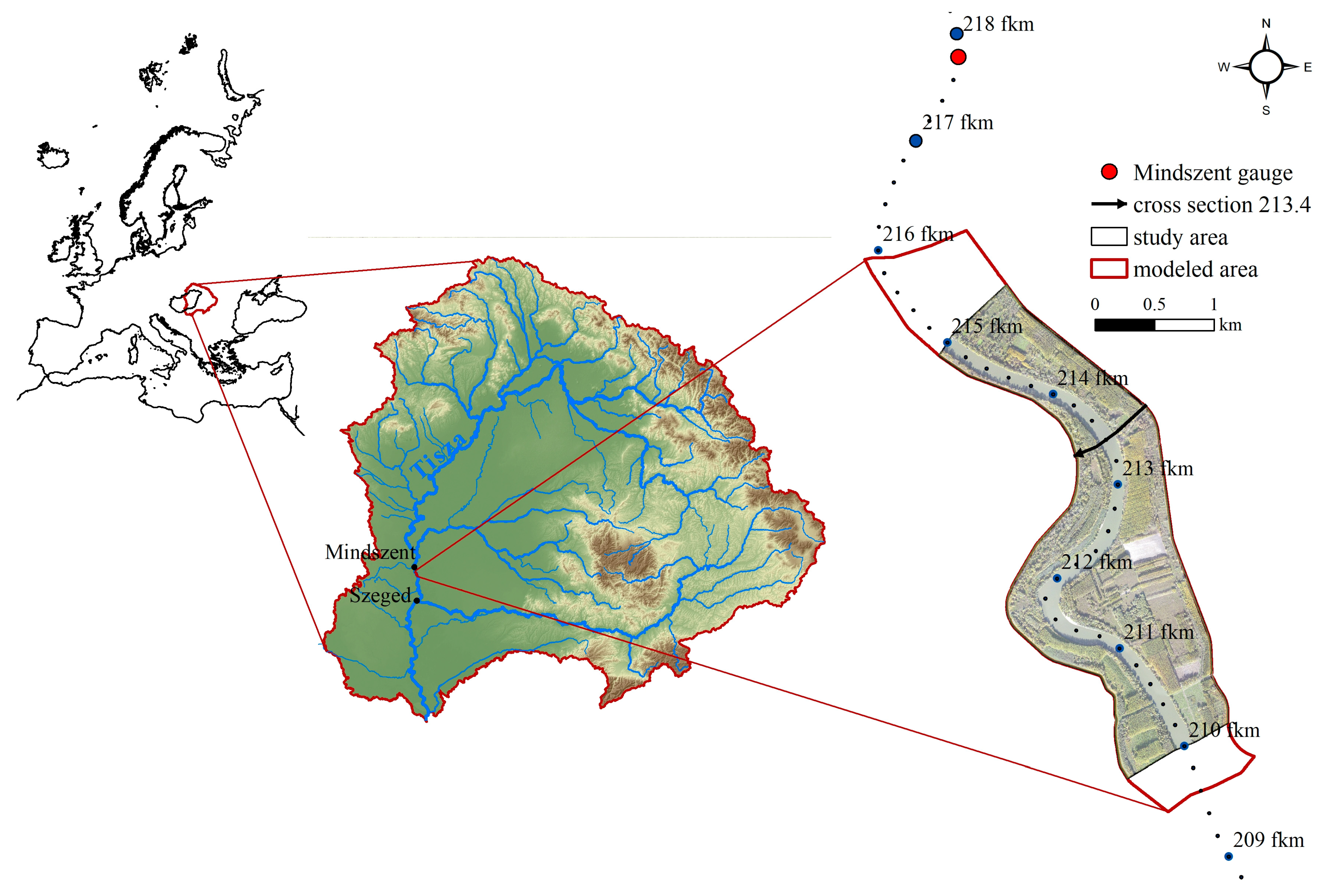
2.1. Study Area

Along the Tisza River (catchment area: 157,200 km2; length: 962 km) in Central Europe (Figure 1), the 5–10-km-wide natural floodplain was confined by artificial levees to 1–4 km in the mid-19th Century [34,77,78]. Ever since, the floodplain has been gradually altered by semi-natural processes. The original wetlands quickly disappeared after the river regulation works, as the channel incised by 3–4.6 m (max 45% increase), and the originally six-month-long floods shortened to 1–3 months [34,76,77,78]. The wetlands were replaced by meadows and plough fields, but by the late 20th Century, even these traditional land uses were abandoned as intensive animal husbandry moved to the villages, and the increasing flood levels destroyed the crops; thus, the farmers ended the cultivation of their lands. In the 1970s and 80s, forest plantations became widespread; thus, today, poplar and riparian willow forests cover 76% of the floodplain [76,77]. Between 1998 and 2006, some extremely high and long floods supported the spread of invasive species (e.g., Amorpha fruticosa, Vitis vulpina, and Echinocystis lobata). These centurial vegetation changes resulted in a 2-4-fold increase in vegetation roughness [76,77] and changed the spatio-temporal pattern of overbank accumulation [34].
The study was performed on a 5-km-long section (210–215 fluvial km) of the Lower Tisza, where the artificially confined floodplain is 0.7–1.5 km wide with a slope ≤2.9 cm/km (Figure 1). Since the beginning of the 20th Century, along this section, the originally 160–220-m-wide channel became narrower (120–160 m), increasing the flood levels by 30–70 cm. The accelerated aggradation increased the food levels by a further 0.3–1.9 m [34].
Just upstream of the study area is a gauging station (Mindszent), where stage measurements were performed. From the start of the measurements (1900), the peak flood level increased by 220 cm. Thus, the highest flood on record in 2006 had already reached the top of the artificial levees. The declining flood conveyance of the channel and the floodplain was well presented by the fact that the increasing flood levels have contributed to the decreasing peak discharge [79]. Downstream of the study area, at Szeged (Figure 1), the peak flood level was 923 cm with 4346 m3/s discharge in 1932, but during the 1970s, the discharge dropped to 3820 m3/s (−12%), but the peak water level increased by 36 cm to 959 cm. The situation became even worse in 2006, when 3780 m3/s contributed to a 1009-cm peak flood level; thus, the peak stage increased by a further 50 cm [34,80]. The 2006 flood was exceptional, the highest flood on record, as the peak flood level reached the top of the artificial levees. Thus, in 2006 the flood protection costs were ca. 120 million USD (0.6% of the annual GDP of Hungary) [81]. Since then, only two small overbank floods have been recorded (2010 and 2013), and the last decade was flood free.
The vegetation is quite dense in the selected section of the Lower Tisza at Mindszent. According to our previous measurements [76,77,78], within a century, the meadows were replaced by planted (43%) and riparian forests (31%), and only 13% of the original meadows and plough fields remained. Moreover, as the study area is located very close to the town of Mindszent, fruit and vegetable gardens were on the floodplain but, due to their gradual abandonment, invasive plants colonised them. Thus, today, Amorpha thickets occupy 13% of the area.
The false indigo (Amorpha fruticosa L.) originated from North–East America and rapidly spread on the floodplain of the Tisza after World War II [82]. Its invasion was related to the end of traditional floodplain farming (grazing) and extensive forestation. The false indigo can seriously inhibit forest renewal, as it overgrows the native plants. Without clearance, it spreads very rapidly, and monodominant stands develop. Under the impenetrable false indigo thickets (height: 3–4 m), the native plant species cannot survive. The habitat becomes unsuitable for animals; thus, the fauna of homogenous false indigo stands is very poor, almost impassable for larger mammals, and unsuitable for nesting or hunting birds. Moreover, the false indigo weakens the artificial levees by its root system and blocks canals and crevasse channels.
Other invasive plants, including wild grape (Vitis vulpina L.) and wild cucumber (Echinocystis lobata Torr. et Gray), also originate from North America, and their invasions started in the first half of the 20th Century [82]. Both plants are lianas, climbing high (>8 m) in the canopy. Their disadvantageous effects include shading, pressing down the native vegetation, and decreasing the biodiversity of the habitats.

2.2. Methods

The vegetation density was determined by analysing the reflectance ratios using the NRD method [63]. The effect of vegetation density on water level and overbank flood velocity was modelled in HEC–RAS 2D for the highest flood on record (2006). The model calibrated for the 2006 flood wave was validated for the 2000 flood wave based on water levels, while water velocities were validated based on actual flow velocity data measured at different points of the floodplain during the 2006 flood by Sándor [83].

2.2.1. Vegetation Density of the Submerged Vegetation Based on the LiDAR Survey

A detailed analysis of the LiDAR data provides an opportunity to evaluate the density of the to-be-submerged understory vegetation over a large area based on a uniform calculation method. We calculated the reflectance per meter for the vegetation density in different height (submerged) zones. The NRD method was used to infer the vegetation roughness in the height zones of interest.
First, the necessary steps for processing the LiDAR data (format conversion, data quality control) were performed. Then, the point-to-cloud reflectance ratios were calculated for the different height zones (1–2 m; 2–3 m up to 4–5 m) at a 15 × 15 m resolution (fitted to the largest canopy diameter) using the DensityMetrics function of the Fusion software. The input data were the elevation model and the LiDAR point cloud. The density calculation was based on the reflectance ratios of the different height zones applying the NRD method [63,73]. To calculate the vegetation density in a given height zone, the number of points reflected from the vegetation height zone under study was divided by the total number of points reflected from and below the given height zone. The calculations were performed for each vegetation height zone on a metered basis. However, only the zones between 1 and 5 m above the surface were analysed in detail, as a record-high overbank flood could submerge these vegetation zones. Thus, their vegetation density could influence the overbank flow velocities during a flood event.
The distribution analysis of the density data (NRD) was performed to determine the vegetation density categories. As a first step, the density values and their corresponding frequency values were plotted on a histogram. The histogram showed that the distribution has a highly skewed peak (towards values < 0.1). According to Francisci [84], such highly skewed distributions could be categorized using class boundaries following the geometric distribution. When defining class boundaries based on the geometric distribution, the class boundaries follow a geometric sequence that distributes the data as evenly as possible into a fixed number of categories. Based on the distribution curves and field observations, the class boundaries were generated at the maximum values of 1, 2, 4, and 16% of the data series, resulting in density classes shown in Table 1.
The probability of inundation and the return period of floods submerging a given vegetation zone were also calculated. The Gringorten formula was used based on the time series (1901–2022) of water stages measured at the Mindszent gauge station, just at the upstream end of the study area (Figure 1).
T   =   n   + 0.12 m   0.44
where T is the recurrence interval of floods, n is the total number of years of record, and m is the magnitude or rank of a given flood.

2.2.2. Hydrodynamic Modelling in HEC–RAS 2D

To model the effect of vegetation density on flow conditions (water levels and flow velocity), the HEC–RAS 2D model was used. The HEC-RAS software was developed at the Hydrologic Engineering Center (HEC), an Institute for Water Resources division, U.S. Army Corps of Engineers. HEC-RAS can perform two-dimensional (2D) hydrodynamic modelling under unsteady, supercritical, or subcritical flow conditions. Thus, detailed 2D channel and floodplain modelling could be performed [85]. The model was calibrated for the record-high 2006 flood. Water levels were validated with the second-largest flood wave in 2000, and at-site flow measurements validated water velocities during the 2006 flood [83].

Geometric Data of the Model

The model was built by integrating the geometry data (topography, roughness, and artificial structures), specifying the hydrological boundary conditions (water level and discharge), performing the calibration runs, and validating the model. The model geometry was based on a terrain model (spatial resolution: 1 × 1 m) that included the elevation of the floodplain and the channel. The resolution of the 2D computational grid mesh in the geometry structure is key to the stability of the model, and it influences the precision of the modelled hydrological processes. Thus, based on test runs, a 10 × 10 m computational grid mesh was defined for the study area.
Manning’s roughness coefficient depends on different environmental factors [42], such as bed material, bed surface, vegetation, bed contour, quantity and quality of transported sediment, and built-in structures (e.g., bridges, embankments). The mean vegetation roughness value for each vegetation density class for the 1–5-m vegetation zone was assigned by applying values published by various authors [42,75,76,83,86]. Thus, the following roughness values were applied: channel n = 0.025, open surface n = 0.02, sparse vegetation n = 0.04, medium dense vegetation n = 0.08, dense vegetation n = 0.016, very dense = 0.2.

Model Scenarios

To evaluate the effects of various management methods of the riparian vegetation on flow conditions, four scenarios were created:
  • The base scenario (S_base) corresponds to the actual state of the floodplain vegetation. It includes the spatially assigned roughness values based on the vegetation density classes calculated from the LiDAR data.
  • The next scenario (S_maintained) represents a state when the actually dense (n = 0.16) and very dense (n = 0.2) understory vegetation patches dominated by invasive species are maintained by invasive plant control. Thus, the vegetation roughness in these patches is reduced to n = 0.08. This scenario represents the most reasonable compromise for the future, as it assumes that the very high areal proportion (ca. 80%) of invasive species is artificially reduced in the floodplain forests.
  • In the least advantageous scenario (S_invasive), the vegetation conditions would deteriorate further, due to the further expansion of invasive species, abandonment of plough lands, and without proper management of planted forests. Thus, patches with very dense undergrowth (n = 0.2) would replace patches with dense (n = 0.16), medium (n = 0.08) and sparse (n = 0.04) undergrowth.
  • The scenario with the lowest roughness (S_meadow) assumes that meadows with low grass cover the floodplain. Thus, over the entire floodplain, the roughness is 0.06. This scenario represents a significantly different state from the actual one; however, it represents 19th Century (pre-regulation) conditions, when marshes and grassy wetlands covered the study area according to the First Military Map (1763–1787).

Hydrological Boundary Conditions of the Model

The model covered the period from 5 April to 5 May 2006, when the floodplain was entirely inundated. During this flood, the highest water level on record reached almost the top of the artificial levees and covered the floodplain with up to 5-m-deep water. At the study area at Mindszent, no discharge data are available. Thus, water level data measured at Mindszent and discharge data were used from a model calibrated by the Middle Tisza Hydrological Directorate for the 2006 flood wave (±5 cm). The upper boundary condition was discharge, while the lower boundary condition was water level. Since the output data of the model were velocity conditions, the SW Momentum algorithm with the full equation SW Momentum was used, which is capable of modelling complex flow conditions with increased computational power.

Calibration of the Model

The calibration of the model was based on the water level measurements along the artificial levees at the peak of the 2006 flood. During the runs, the recorded water levels’ elevation and the model’s calculated ones were retrieved and used to generate a hydrograph (Figure 2). The model adequately represents water levels, though deviations (−9 cm) in the upstream section of the modelled area exist due to the small model area, the extremely low slope (≤2.9 cm/km) of the river, the effect of the reduction of the grid resolution (10 m), and the uncertainties of the water level measurements. Therefore, the flow conditions were analysed in detail in the central part of the modelled area (Mindszent: 215–210 fluvial km), where the accuracy was within ca. 5 cm.
The calibration also included a sensitivity analysis of the different understory density categories. The initial value was determined based on Sándor [83], and the sensitivity tests were performed by increasing and decreasing the roughness values for each category by 20%.

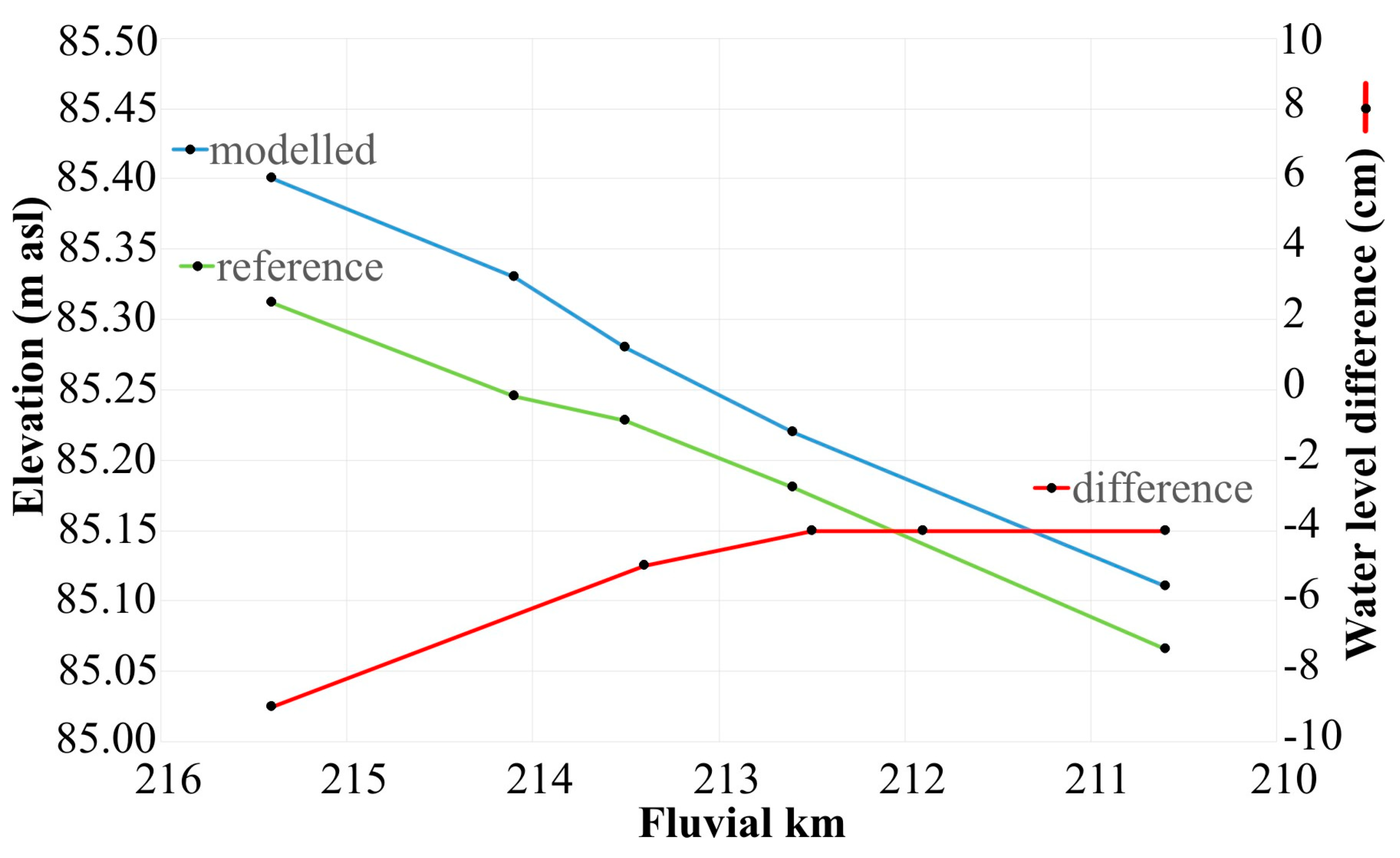
Validation of the Model for Water Level

The calibrated model was validated using hydrological data at the peak of the 2000 flood. For the validation, the model data calibrated by the Central Tisza Region Water Directorate (KÖTIVIZIG) for the 2000 flood event were used as boundary conditions. Furthermore, the land-use data based on an orthophoto taken in 2000 (resolution: 10 cm) were applied. To verify the calculated results, water level measurements made in 2000 along the artificial levee during the flood peak were used.
Despite the close temporal proximity of the flood waves and the similar peak stages, the control fit (2000 flood water level recordings and modelled water levels at the peak of the 2000 flood) did not give a good match, as the differences exceeded 20 cm at several points (Figure 3). It could be reasoned by (1) the difference in mean water depths during the studied flood waves and (2) the increase in vegetation density between 2000 and 2006. Since the energy loss caused by vegetation in the flow path is proportional to the surface area exposed to the flow, lower water depths are expected to result in lower energy loss; i.e., a lower roughness coefficient. Considering this, Manning’s (n) roughness coefficient values determined for the forested areas during validation were uniformly reduced. After this adjustment, the measured and calculated water levels along the entire length of the studied section showed very good correspondence, with differences of less than 10 cm (root mean square error: 5.5 cm).

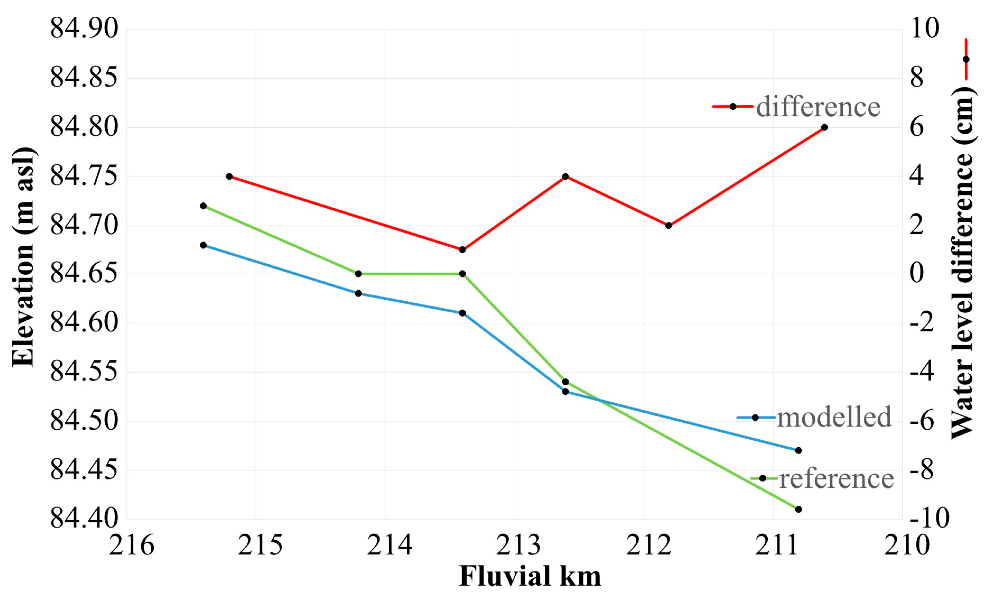
Validation of the Model for Flow Velocity

The model was validated not only for water level but also for flow velocity at 23 points in 90-cm depth. The flow velocity measurements were made on the eastern floodplain area of the study site by A. Sándor and T. Kiss during the peak of the 2006 flood [83]. The measurements were made with a calibrated GR-21 flow velocity meter, which accurately measures the velocity in the range of 0.14–2.86 m/s.
The mean difference between the modelled and measured velocities was 0.1 m/s, which, considering the instrument’s accuracy, was considered as good. The largest deviation was 0.3 m/s (modelled 0.42 m/s instead of measured 0.12 m/s), but there were 6 points where the differences were within ±0.01 m/s.

3. Results

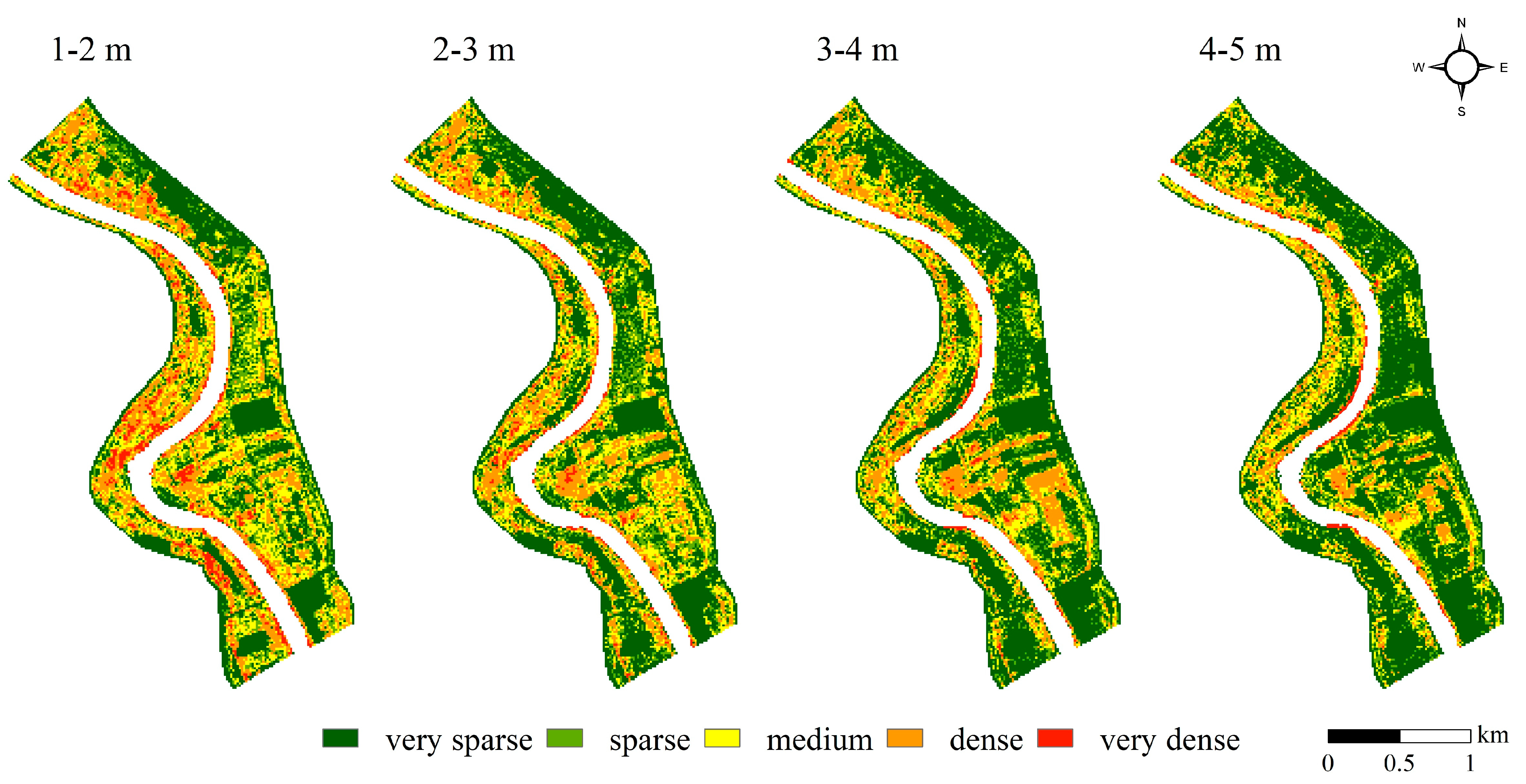
3.1. Vegetation Density of the Submerged Vegetation Zones

On the floodplains of low-gradient rivers, the overbank flow velocity is low; thus, the obstacles in the flow path can substantially alter flow conditions. Since the artificial levees along the confined floodplain of the Tisza have an average height of 5 m, the vegetation density of the 1–5-m height zone was the focus of our study, as during the highest floods (which reach the top of the levee) this vegetation zone is inundated.
Diverse vegetation patches with various density conditions were identified in the studied floodplain section (Figure 4). In the narrow, western floodplain section, the vegetation is dense or very dense; though, in some patches, the vegetation was cleared for young poplar plantations.
The wide eastern floodplain has spatially diverse riparian vegetation. In its upstream part, near the levee, sparse understorey poplar plantations occur, and riparian willow patches with dense understorey appear towards the channel. In the middle part of the floodplain, poplar plantations were identified with very dense understorey invaded by Amorpha along the levee and with low to medium vegetation densities along the river bank. On the downstream part of the eastern floodplain, mostly abandoned gardens and agricultural fields with very dense Amorpha thickets were identified (rectangular pattern), and only some plough land mosaics and medium-density poplar plantations occur. Along the river, riparian willow forests with dense undergrowth are common.
Overbank flood waves submerge the vegetation of the 1–2-m height zone approximately every second year, when the water level at the Mindszent gauging station is 600–700 cm. In this height zone, dense (23%) and very dense (5%) understorey patches are common (Figure 4, Table 2). The vegetation is especially dense in abandoned gardens, fallow agricultural fields, and unmanaged forests. In contrast, patches with very sparse (38%) and sparse (12%) undergrowth cover 50% of the area. Such patches are mainly found in the middle of the eastern floodplain, where crops are planted on some large plots and the poplar forests are managed by clearing the understorey bushes.
The 2–3-m height vegetation zone is inundated by 700–800 cm floods with a return period of ca. three years. In this zone, the proportion of dense (20%) and very dense (2%) undergrowth decreases by 6% compared to the 1–2-m zone, while the very sparse vegetation became more common (44%). Thus, in terms of overbank flow, this zone can convey floods more effectively than the lower, 1–2-m height zone.
The 3–4-m vegetation zone is flooded every 9 years by 800–900-cm high stages, whereas the uppermost, 4–5-m vegetation zone is rarely submerged (return period: 25 y) by record high floods (>900 cm). In these zones, the proportion of dense and very dense understorey patches is lower (3–4 m: 15%; 4–5 m: 10%), as they are replaced by low-density or vegetation-free cells.

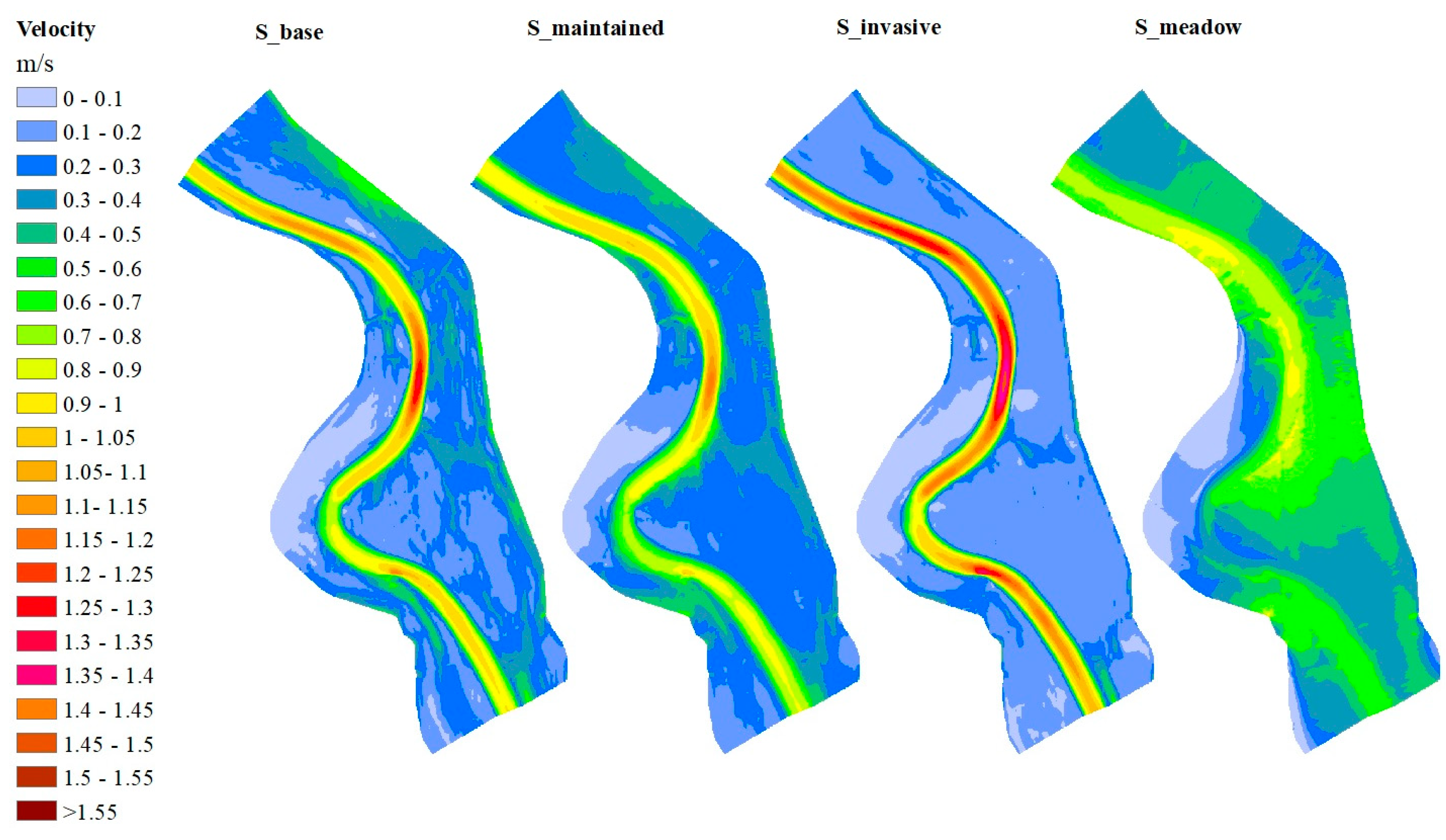
3.2. Spatial Distribution of Flow Velocity Fields in Different Scenarios

Based on the vegetation density map, a vegetation roughness map was created by applying the vegetation roughness values determined by Chow [42], Sándor [83], and Nagy et al. [76]. The created vegetation roughness map was input data of the 2D hydrodynamic model; thus, the effect of vegetation on flood flow conditions could be quantified (Figure 5).
The S_base scenario represents the actual vegetation and flow conditions. Along the banks, in the vegetation with dense understorey, the flow velocity of the overbank flood is below 0.1–0.2 m/s, even during the peak of the flood. This zone with high vegetation roughness forces the flow towards the eastern artificial levee. Thus, in between them, in the sparse poplar plantations and especially in its low-lying areas, the flow accelerates to 0.5–0.6 m/s, creating a well-visible flow path in the middle of the floodplain. Under these circumstances, the tree lines of the plantations can effectively influence the overbank flow. In the channel, the flow velocity is 1–1.1 m/s. The water enters the floodplain at several points through crevasses. One of the crevasse channels conveys the flood flow through a swale to the middle of the floodplain to a plough field, where the overbank flow velocities reach 0.4–0.5 m/s. In contrast, the water flow slows to 0.1–0.2 m/s in areas with dense and very dense undergrowth.
In the S_maintained scenario, the management of the undergrowth vegetation (e.g., clearance of invasive species) improves the vegetation roughness, especially in the near-bank zone. Therefore, the flow velocity increases to 0.2–0.4 m/s along the bankline and decreases to 0.3–0.5 m/s along the artificial levee. The crevasses merge to form a wider strip where the overbank flow velocity reaches 0.5–0.6 m/s. In this scenario, the in-channel flow velocity decreases to 0.8–1 m/s.
As the dense undergrowth with invasive species spreads over the floodplain (S_invasive), the flow velocity decreases to ≤0.1 m/s on the entire floodplain. The overbank flow is almost uniformly stagnant all over the study area. Thus, no distinct conveyance zone is formed, and the activity of crevasses is very limited. On the contrary, the flow velocities in the channel increase to 1.2–1.3 m/s, and areas of pronounced high velocity (1.4 m/s) develop in the northern meander (Figure 5).
The S_meadow scenario represents a much lower vegetation density and roughness than the current conditions. In this scenario, the overbank flow enters the floodplain through crevasses (e.g., in the lower third of the upstream meander). Thus, high flow velocities (0.5–0.7 m/s) evolve over the entire floodplain. Since vegetation does not block the crevasses, they merge, creating a wide flood conveyance zone. This conveyance zone extends to the artificial levee, and in its widening section, the maximum flow velocity reaches 0.8 m/s. In the low-lying areas of the floodplain, the flow velocity also accelerates (0.5–0.6 m/s). Meanwhile, in the channel, the lowest water velocities of all scenarios prevail (0.6–0.8 m/s).
On the downstream part of the western floodplain, low flow velocity fields form in all scenarios. Its development is influenced by the remnants of a 19th Century artificial levee running perpendicular to the channel. It effectively blocks the overbank flow; therefore, in all scenarios, the flow velocities are ≤0.1 m/s.

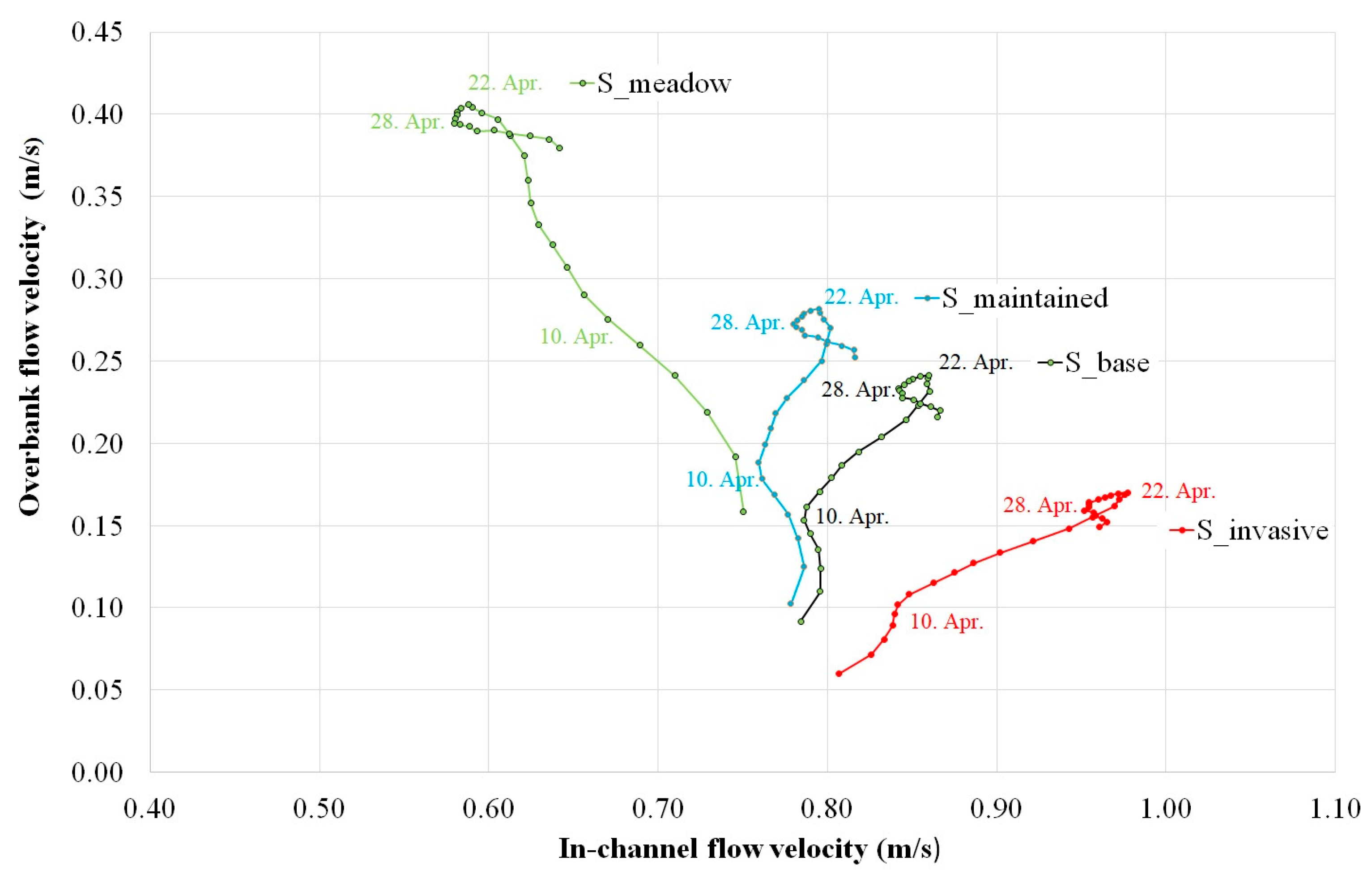
3.3. Temporal Changes in Overbank Flow Velocities in Different Scenarios

The 2D hydrodynamic model made it possible to analyse and compare the flow conditions during the subsequent phases of the 2006 flood, i.e., during the rising limb (5–21 April 2006) when the stages increased from 747 cm to 1061 cm; during its peak (22 April 2006), when the Tisza reached its highest level on record (1062 cm) and reached the top of the levees at some points; and finally, during its falling limb (23 April–5 May 2006) when the impoundment by the Danube terminated, and the Tisza could start to drop.
In the actual situation (S_base), on the first day of the modelled period, the floodplain was already covered by a 2-m deep water column, and the mean overbank flow velocity was 0.09 m/s. During the rising limb, the flow velocities increased, as the 0–0.3 m/s velocity field covered 81% of the study area. During the peak of the flood, the mean inundation depth was ca. 5 m, the mean overbank flow velocity increased by 2.6 times to 0.24 m/s, and the maximum flow velocity was 1.3 m/s. Even during the peak, the overbank flow was relatively slow on the floodplain, as flow velocities ≤ 0.3 m/s appeared on two-thirds of the study area. During the falling limb, the drop of stages was slow; thus, the changes in average floodplain velocities were also moderate: in two weeks the average velocity (0.21 m/s) only decreased by 13%. The proportion of areas with low flow velocities (0–0.3 m/s) increased to 69%, while the proportion of areas with higher water velocities gradually decreased (Table 3).
In the case of invasive plant management (S_maintained), the flow velocities only differ by 1–2% from the base situation. At the peak of the flood, the mean flow velocity increases to 0.28 m/s, thus, by 16% compared to the S_base situation. The maximum flow velocity (1.1 m/s) on the day of the peak is slightly less than for the base scenario (1.3 m/s). However, the proportion of medium (0.3–0.6 m/s) and high (>0.6 m/s) flow velocity fields significantly increases during the peak. During the falling limb, the water level decrease remains slow due to the nature of the flood wave (impoundment by the Danube). However, on the last day of the modelled period, the average velocity is still 17% higher than in the base scenario. Thus, vegetation maintenance reduced the proportion of low flow velocity fields during the peak and the falling limb of the flood wave and increased the proportion of higher water velocities (≥0.3 m/s).
The worst flood conveyance conditions develop in the absence of vegetation management, when the forest understorey is dense, and the fallow lands are invaded by invasive species (S_invasive). In this case, at the beginning of the flood, the mean overbank flow velocity decreases to 0.06 m/s, being one-third lower than in the S_base. In the rising limb, there is only a 1–2% difference between the S_invasive and S_base scenarios. At the peak of the flood, there is a 30% velocity drop due to dense vegetation. This velocity difference also remains in the falling limb when the mean floodplain velocity drops to 0.15 m/s, being lower than the S_base by 28%. This implies that the extent of low flow velocity (<0.3 m/s) fields during the peak and the falling limb significantly increases, and higher velocities only appear in small patches.
In the case of floodplain restoration, when the study area is completely covered by meadows and open surfaces (S_meadow), the mean flow velocity could be 0.16 m/s on the first day of the flood; thus, it is doubled compared to the S_base. In this scenario, the proportion of medium and high flow velocity fields increases by 3–4%, and a zone with high overbank flow velocity also evolves. At the peak of the flood, the mean flow velocity over the floodplain increases to 0.41 m/s, which is higher than the velocity conditions of the S_base by 70%. The area of the low-flow velocity fields significantly decreases, while the medium- and high-velocity flow fields become dominant. However, the maximum velocity decreases, and it reaches its lowest value (1 m/s). During the falling limb of the flood wave, the mean overbank flow velocity decreases from 0.41 m/s to 0.38 m/s in two weeks, which is 80% higher than the value of the reference scenario.

3.4. Temporal Changes in In-Channel Flow Velocities in Different Scenarios

The flow velocity in the channel is closely related to the flow velocity in the floodplain, as models reflect their complementary character: as the overbank flow velocity in the floodplain increases, it decreases in the channel.
The temporal connection between the mean overbank and in-channel flow velocities could be described by a loop-like curve (Figure 6). During the first part of the loop (5–10 April; H: 747–848 cm), the in-channel flow velocities moderately vary, while an intense increase in overbank flow velocity could be observed. It can be explained by the gradual spread of the flood wave over the floodplain. After the flood wave covers the entire floodplain and slowly reaches its peak (11–22 April; H: 873–1062 cm), the in-channel flow velocity increases more and more intensively as a function of vegetation roughness. The greater the vegetation roughness of the floodplain, the more intensive the velocity increase rate in the channel, causing the loop curves to rotate counter-clockwise. For example, in the S_meadow scenario, the flow velocity in the channel decreases as the flood progresses. After reaching the peak in the third period (23–28 April; H: 1060–1036 cm), the falling limb slowly starts. At this time, both the in-channel and overbank flow velocities are reduced, and the curve inverts. In the last part of the flood wave (after 29th April; H: <1028 cm), the flood conveyance in the channel becomes more intensive as the impoundment by the Danube ceases. Thus, in-channel flow velocities start to increase, while overbank flow velocities slowly decrease.

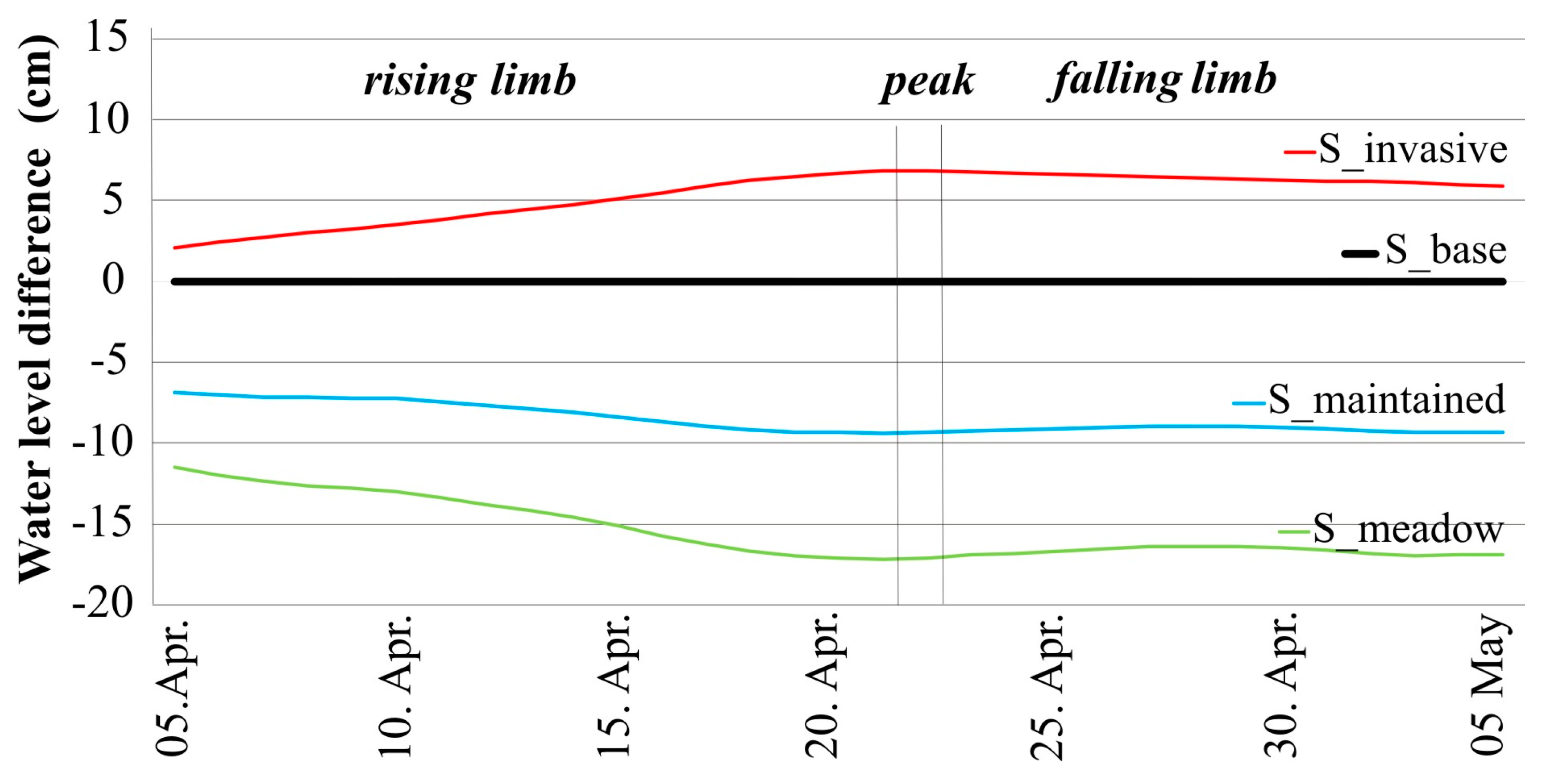
3.5. Changes in Water Levels in Different Scenarios

Based on the modelled data, the differences in water levels were analysed for a transect in the middle of the study area (213.4 fluvial km; Figure 1 and Figure 7). In the case of managed understorey vegetation (S_maintained), the water levels are lower by 7 cm than in the case of S_base at the beginning of the flood wave. However, as the flood rises, their difference steadily increases, reaching a 10-cm difference during the peak of the flood. It indicates that forest maintenance could achieve a 10-cm decrease in peak water levels. During the falling limb of the flood, this difference remained at 9 cm.
Due to the extremely dense vegetation (S_invasive), the water levels only exceed the S_base stages by 2 cm at the beginning of the rising limb. However, during the peak, their difference increases to 7 cm, however, and it remains at 6 cm during the falling limb.
Thus, the comparison of the above-presented scenarios (S_maintained and S_invasive) shows that the further spread of invasive species could increase the flood stages by just 2–7 cm, while the maintenance of vegetation could reduce water levels by 7–10 cm compared to the actual situation.
On the contrary, if pastures and meadows could be restored in the floodplain (S_meadow), even at the beginning of the flood the water levels could decrease by 11 cm compared to the S_base. At the peak of the flood, the water level difference is already 17 cm, and it slightly decreases to 16 cm during the falling limb (Figure 7).

4. Discussion

From the point of view of hazard management, the primary function of the low-gradient, lowland rivers is to support the propagation of flood waves and to provide fast and safe flood conveyance without levee breaching or overtopping. According to our hypothesis, the submerged vegetation’s spatial dimensions (vertical and horizontal) fundamentally influence the flow conditions (e.g., velocity, directions) and height of flood waves.

4.1. Riparian Vegetation Density with Special Respect to the Submerged Vegetation Zones

Due to the centurial changes in riparian vegetation cover along the Tisza River [76], today, the mean vegetation density is quite high (NRDmedian: 0.007–0.051) in the area, especially in the lowest inundation zone, in the Amorpha thickets [78]. Our NRD results provided very similar data to the results of point-like density measurements performed by Sándor [83] and Delai et al. [75] in the same area. However, applying the LiDAR dataset as a source and the NRD as a method, the vegetation density of the entire study area could be evaluated, thus spatially detailed roughness data for the 2D modelling could be provided.
In the study area, the vegetation is the densest in the lowest (1–2 m) flooded zone, and upward in the higher zones it becomes thinner [78]. Thus, in the 1–2-m zone, the proportion of very dense and dense vegetation is 28%, but it decreases to 10% in the uppermost (4–5 m) zone. Simultaneously, sparse or very sparse vegetation occupies 50% of the territory in the lower zone, but their proportion increases to 78% in the uppermost zone [78]. Thus, the propagation of smaller flood waves (H: <800 cm, return period: ≤3 y) or the rising stages of the larger flood waves are more influenced by the dense vegetation than the peak periods of the extreme high floods.
Comparing the spatial distribution of vegetation density classes to vegetation types of the floodplain [78], it should be noted that the dense and very dense patches are common under the natural willow forests and in the Amorpha thickets. As the willow forests are along the banks, where the channel narrowing created new areas [79] to be colonised by natural riparian forest, the near-bank zone has high vegetation density, thus high vegetation roughness, unfavourably influencing the flood conveyance. Moreover, the canopy structure and the relatively short lifetime of the Salix species [87] provide good light conditions for the growth and spread of invasive plants, such as Amorpha, which further deteriorate the flood conveyance of these patches. Along the sharp southern bend, fallow agricultural parcels and abandoned gardens occur, and dense Amorpha thickets occupy them. As these plants are usually 3–4 m high, they increase the vegetation density in the lower zones, effectively blocking the overbank flow in the chute of the meander.

4.2. Hydrological Consequences of Vegetation Changes

The submerged Amorpha thickets effectively impede overbank flood flow. It was also supported by our former, point-like velocity measurements [79] during the peak of the 2006 flood: within the thickets, the flow velocity was 0 m/s, but above them, it was 0.13 m/s. However, our modelling proved that the spread of invasive plants is especially problematic along the banks where the flood enters the floodplain and along flood conveyance zones in the distal, deep-lying areas. The situation is especially critical along the southern, sharp meander. Here, on the eastern part of the floodplain, the very dense vegetation effectively delays the flow. In contrast, on the western side, the remnants of a 19th-Century artificial levee (perpendicular to the flow) block the overbank flood. Moreover, the sharp meander also slows down the flood wave. Thus, here, the increase in flood levels due to local reasons is expected.
The four modelled scenarios reflect gradual vegetation changes in the floodplain and its hydrological consequences. Thus, the subsequent scenarios could be used to interpret the historical changes in flood conveyance: The S_meadow scenario reflects the vegetation conditions before the 19th-Century regulation works when only meadows and wetlands covered the floodplain. Then, the S_maintained represents the stage in the mid-20th Century when invasive species have not been on the floodplain yet, but already forests have become widespread due to extensive plantations. The S_base reflects the actual situation, and the S_invasive predicts the changes if everything goes on as usual, so no invasive plant control will be made.
In the scenario reflecting 19th-Century conditions (S_meadow), channel morphology, relief, and floodplain width were the most important factors influencing the overbank flood flow velocity and directions, as the vegetation was spare and mainly herbaceous. Upstream of the meander’s axes, the flood could easily enter the floodplain in a wide (crevasse) zone, and the flood conveyed in the chute of the meanders. However, as the vegetation became denser on the floodplain in the 20th Century (S_maintained and S_base), it could effectively obstruct the flood flow entering the floodplain. Thus, the crevasse zone became gradually narrower and the overbank flood velocity became slower. In the future, when the invasive species (S_invasive) are likely to invade the floodplain more than today [88], these crevasses will almost stop functioning. As the vegetation grows denser, the flow velocity in the thickets of the floodplain will be almost zero. Thus, most of the water will be conveyed within the channel, and if the flood is high enough, water movement will be detectable just above the densest vegetation zone (1–3 m).
Increased vegetation density and the spread of invasive plants have already affected flood levels and safety. Since the beginning of the 20th Century, the peak flood levels have considerably increased (by 220 cm), which means that the artificial levees have had to be heightened to provide flood safety. According to our results, since the 19th Century, the increased vegetation density is responsible for a 17-cm flood level increase. If the vegetation grows even denser, a further 7 cm could be expected. As the 2006 flood reached the top of the levees at some locations, it is urgent to develop an action plan to control invasive plants or re-plan the vegetation patches to support overbank flood conveyance.
On the other hand, the result of the 2D modelling is quite contradicting, as our previous 1D modelling indicated a 42–139-cm flood level increase due to the dense vegetation [34,77,80]. The difference probably originates from the different study area sizes (1D: 350 km; 2D: 6 km) of the models. Suppose a modelled area managed by invasive plant control is embedded into a larger floodplain area with dense riparian vegetation. In that case, there is a considerable drop in stages, increased velocity at the upstream end of a managed area, and significant impoundment at the downstream part (1–2 km) as the flow enters the next impenetrable vegetation [77]. If the modelled (managed) area is long enough, these upstream and downstream effects become negligible (like in our 1D modelling); however, in the case of short sections, the effects overlap.
The decreased overbank velocities influence the overbank aggradation rate. As the Tisza transports a large amount of suspended sediment [89], the gradually declining flow velocities could support increasing aggradation. The role of vegetation in overbank aggradation has been emphasized by several researchers [34,78,80,83,90]. It must also be noted that the increased sedimentation will further contribute to flood level increase [34,80]. Thus, the vegetation indirectly further decreases the flood conveyance of the confined floodplain.
The modelling also supported that the maximum in-channel flow velocity increased from 1.0 m/s (S_meadow) to 1.3 m/s (S_base), and in the future, it will likely further increase to 1.4 m/s (S_invasive). The increased velocity increases the shear stress on the channel. On the other hand, the dense vegetation blocks lateral erosion and channel widening. Thus, the Tisza is already incised, and the process will likely continue. As a result of the ongoing incision, the point bars have already disappeared [91], and the level of the lowest discharges has dropped [80], triggering the drop in groundwater level, which generated the aridification of the nearby areas [88,92]. As the floodplain becomes drier, the spread of invasive species will be further supported, whereas the hygrophilous native plants disappear. Thus, in the future, further channel incisions could be predicted. However, the incision will probably not reduce the overbank flow as it has been reported on other rivers [93] because the incision of the Tisza is surpassed by considerable channel narrowing and cross-sectional area decrease [79,80].
The hydrological model also highlighted another zone where the flow velocity increases: along the artificial levees. Low vegetation density grassland is maintained in a ca. 10-m-wide zone by the feet of the levees. In this zone, the flow velocity is high (S_base: 0.4–0.7 m/s), which endangers the stability of the levees built of silt and clay [94], thus they could be eroded by the flow.
All these direct and indirect hydro-morphological processes increase the flood levels and decrease flood safety [34]. They also support the further spread of invasive plant species and the appearance of new ones. The extremely dense, already impenetrable riparian vegetation increases other hazards as well, including fire hazard [69], aggradation of microplastics and other pollutants in the sediments, and the trapping of macroplastics in the riparian vegetation [95].

4.3. Suggestions for Sustainable Flood and Riparian Vegetation Management

Proper riparian vegetation management could mitigate the unfavourable hydro-morphological changes related to vegetation density. The vegetation density should be decreased by removing invasive species and replacing forests with meadows at some key locations. These measures would also be favourable from the perspective of biodiversity. The invasive species widespread on the Tisza floodplain are bushes or lianas shading the original habitats and suppressing shorter plants. Moreover, the Amorpha impedes the germination of other seeds and causes serious problems in the renewal of riparian forests [82]. Therefore, the clearance of these invasive species would be necessary, both from hydrological and ecological points of view. Furthermore, the re-created open riparian habitats (e.g., meadows and pastures) could support diverse flora and fauna [88].
The modelled scenarios highlighted those areas where the management should be the most important: along banks where the flood enters the floodplain and in flood conveyance zones (deep-lying areas) of the floodplain. Therefore, it is suggested to perform similar 2D modelling, especially in areas where the local flood level increase is the greatest, and to highlight those zones which should be managed. Moreover, the maintenance of the riparian vegetation could support not just floodplain management, but also help to stop channel incision and groundwater lowering.
The presented case study was performed on the low-gradient Lower Tisza River (slope: 2.9 cm/km), but the method should be tested on rivers with greater slopes. Our previous HEC-RAS 1D modelling on the Middle Tisza (slope: 3.7 cm/km) and on the Maros (slope: 5 cm/km) proved that as the slope of the floodplain increases, the blocking effect of the vegetation decreases [77].
A pilot project within the frame of the Danube Floodplain Project [40,96] aimed to manage the riparian vegetation at some sites of the Middle Tisza. However, their success is questionable, as here only small patches were managed by grazing, and according to our 1D and 2D modelling, longer (several km long) floodplain sections should be managed, otherwise, it has no hydrological effect. Moreover, these pilot projects were not continued after the end of their financed period, thus, with the lack of financial support, the grazing and the invasive plant control were terminated, and even denser invasive vegetation developed.
Therefore, we suggest creating legislation, similar to the control of common ragweed (Ambrosia elatior), which is also densely spread in Hungary. According to the Hungarian Government decree [221/2008. (VIII. 30.)], every landowner must clear it before flowering unless a considerable fine is paid. Similar legal regulations should also be implemented on the invasive species of the floodplains, which could encourage landowners to reduce vegetation density. Furthermore, educational programs could help local stakeholders to understand the problem and to accordingly act. Continuous maintenance would be especially important, as the invasive species, including Amorpha, have large seed and propagulum production and long seed lifetime (ca. 40 years) [82,87].
It also has to be emphasised that though local initiatives are important, only large-scale vegetation management could result in proper flood conveyance zones on the floodplain and decrease flood levels. If the vegetation will not be managed, other engineering solutions (e.g., heightening artificial levees, channel widening) will be needed to support flood safety.
Another aspect of proper management is up-to-date monitoring. Our study proved that the analysis of a LiDAR survey could provide accurate data on the spatiality of vegetation density of the potentially submerged understorey vegetation. It is a good tool for estimating vegetation density in areas with impenetrable shrubbery. Thus, the critical vegetation patches could be identified by regular monitoring using a LiDAR survey; thus, the areas where maintenance is needed could be identified, and the effect of the maintenance could be evaluated. Only one LiDAR survey was made along the Tisza; thus, no information on the temporal changes in the vegetation density could be provided.

5. Conclusions

The riparian vegetation along rivers is highly affected by climate-change-driven environmental processes (e.g., flash floods, droughts, fires) and various human impacts (e.g., river engineering, forestry). Thus, the vegetation type and composition of the riparian zone gradually change, which alters the hydrological processes. Some regions are especially prone to floristic changes: for example, the floodplains of Central European rivers are highly invaded by invasive plants, which displace the native vegetation. Thus, along the Tisza, almost impenetrable shrubbery has developed, replacing the native meadows and invading the understorey of native and planted forests and fallow lands.
The drastic change in vegetation altered the fluvial processes, as was proven by our 2D modelling. Flow velocities gradually drop, and if the invasive plants are not controlled, and the planted forests further gain space, the floodplain will limitedly convey overbank floods in the future. Therefore, it will act rather like a sponge with stagnant water. As the main hydrological function of the floodplains is to convey floods, these processes are very unfavourable from the point of view of flood hazard management. In our case, the modelled 2006 flood already reached the top of the artificial levees, and ever since, the riparian vegetation has become even denser. Therefore, in the future, a flood with a similar discharge will have higher stages; thus, the levees will be overtopped. It endangers those millions who live along the river and exposes the infrastructure to damage.
Thus, the maintenance plans for the floodplain should be created as soon as possible, considering and fitting the needs of hydrology, ecology, forestry, and land owners.
The 2D model was developed for a low-slope floodplain with impenetrable vegetation invaded by invasive plants. Climate change, fires, acidification, and extreme floods also support the spread of invasive species in other regions. However, to understand their effect on hydrology, the modelling should be performed on floodplains with various slopes, widths, and hydrology.

Author Contributions

Conceptualization, T.K.; methodology, I.F.; writing—original draft preparation, I.F.; writing—review and editing, T.K. All authors have read and agreed to the published version of the manuscript.

Funding

The research was funded by the Hungarian Research Foundation (OTKA 134306 and 119193).

Institutional Review Board Statement

Not applicable.

Informed Consent Statement

Not applicable.

Data Availability Statement

Data available upon request.

Acknowledgments

The authors are grateful for the Lower Tisza District Water Directorate for supporting our research by various data (stage, discharge), and for the LiDAR dataset.

Conflicts of Interest

The authors declare no conflict of interest.

References

  1. Downs, P.W.; Piegay, H. Catchment-scale cumulative impact of human activities on river channels in the late Anthropocene: Implications, limitations, prospect. Geomorphology 2019, 338, 88–104. [Google Scholar] [CrossRef]
  2. Galia, T. Legacy of Human Impact on Geomorphic Processes in Mountain Headwater Streams in the Perspective of European Cultural Landscapes. Geosciences 2021, 11, 253. [Google Scholar] [CrossRef]
  3. Timofte, F.; Onaca, A.; Urdea, P.; Právetz, T. The evolution of Mures channel in the lowland section between Lipova and Nadlac (in the last 150 years), assessed by GIS analysis. Carp. J. Earth Environ. Sci. 2016, 11, 319–330. [Google Scholar]
  4. Rentier, E.S.; Cammeraat, L.H. The environmental impacts of river sand mining. Sci. Total Environ. 2022, 838, 155877. [Google Scholar] [CrossRef]
  5. Bertalan, L.; Rodrigo-Comino, J.; Surian, N.; Šulc Michalková, M.; Kovács, Z.; Szabó, S.; Szabó, G.; Hooke, J. Detailed assessment of spatial and temporal variations in river channel changes and meander evolution as a preliminary work for effective floodplain management. The example of Sajó River, Hungary. J. Environ. Manag. 2019, 248, 109277. [Google Scholar] [CrossRef]
  6. Wyzga, B.; Radecki-Pawlik, A.; Galia, T.; Plesinski, K.; Skarpich, V.; Dusek, R. Use of high-water marks and effective discharge calculation to optimize the height of bank revetments in an incised river channel. Geomorphology 2020, 356, 107098. [Google Scholar] [CrossRef]
  7. Fan, J.; Huang, G. Evaluation of Flood Risk Management in Japan through a Recent Case. Sustainability 2020, 12, 5357. [Google Scholar] [CrossRef]
  8. Lóczy, D.; Kis, É.; Schweitzer, F. Local flood hazards assessed from channel morphometry along the Tisza River in Hungary. Geomorphology 2009, 113, 200–209. [Google Scholar] [CrossRef]
  9. Scorpio, V.; Aucelli, P.C.; Giano, S.I.; Pisano, L.; Robustelli, G.; Rosskopf, C.M.; Schiattarella, M. River channel adjustments in Southern Italy over the past 150 years and implications for channel recovery. Geomorphology 2015, 251, 77–90. [Google Scholar] [CrossRef]
  10. Rusnak, M.; Lehotsky, M.; Kidova, A. Channel migration inferred from aerial photographs, its timing and environmental consequences as responses to floods: A case study of the meandering Topla River, Slovak Carpathians. Morav. Geogr. Rep. 2016, 24, 32–43. [Google Scholar] [CrossRef]
  11. Dragićevć, S.; Pripužić, M.; Živković, N.; Novković, I.; Kostadinov, S.; Langović, M.; Milojković, B.; Čvorović, Z. Spatial and Temporal Variability of Bank Erosion during the Period 1930–2016: Case Study—Kolubara River Basin (Serbia). Water 2017, 9, 748. [Google Scholar] [CrossRef]
  12. Magliulo, P.; Bozzi, F.; Leone, G.; Fiorillo, F.; Leone, N.; Russo, F.; Valente, A. Channel adjustments over 140 years in response to extreme floods and land-use change, Tammaro River, southern Italy. Geomorphology 2021, 383, 107715. [Google Scholar] [CrossRef]
  13. Magliulo, P.; Cusano, A.; Giannini, A.; Sessa, S.; Russo, F. Channel Width Variation Phases of the Major Rivers of the Campania Region (Southern Italy) over 150 Years: Preliminary Results. Earth 2021, 2, 374–386. [Google Scholar] [CrossRef]
  14. Mandarino, A.; Pepe, G.; Cevasco, A.; Brandolini, P. Quantitative Assessment of Riverbed Planform Adjustments, Channelization, and Associated Land Use/Land Cover Changes: The Ingauna Alluvial-Coastal Plain Case (Liguria, Italy). Remote Sens. 2021, 13, 3775. [Google Scholar] [CrossRef]
  15. Liro, M. Impact of channel regulation on sedimentation on the Lower Dunajec floodplains. Prz. Geol. 2012, 60, 380–386. [Google Scholar]
  16. Rădoane, M.; Perșoiu, I.; Chiriloaei, F.; Cristea, I.; Robu, D. Styles of Channel Adjustments in the Last 150 Years. In Landform Dynamics and Evolution in Romania; Springer: Berlin/Heidelberg, Germany, 2017; pp. 489–518. [Google Scholar]
  17. Labaš, P.; Kidová, A. Anthropogenic and environmental impacts on the recent morphological degradation of the meandering Hornád River. Geogr. Casopis. 2022, 74, 159–180. [Google Scholar] [CrossRef]
  18. Timofte, F.; Urdea, P. Three centuries of dynamics in the lowland section, induced by human impact: A sociogeomorphic approach. Geogr. Pannonica 2022, 26, 308–318. [Google Scholar] [CrossRef]
  19. Nádudvari, Á.; Czajka, A.; Wyżga, B.; Zygmunt, M.; Wdowikowski, M. Patterns of Recent Changes in Channel Morphology and Flows in the Upper and Middle Odra River. Water 2023, 15, 370. [Google Scholar] [CrossRef]
  20. Zhou, M.; Xia, J.; Deng, S. One-dimensional modelling of channel evolution in an alluvial river with the effect of large-scale regulation engineering. J. Hydrol. 2019, 575, 965–975. [Google Scholar] [CrossRef]
  21. Zhou, M.; Xia, J.; Deng, S.; Li, Z. Two-dimensional modeling of channel evolution under the influence of large-scale river regulation works. Int. J. Sedi. Res. 2022, 37, 424–434. [Google Scholar] [CrossRef]
  22. Surian, N. Fluvial Changes in the Anthropocene: A European Perspective; Elsevier: Amsterdam, The Netherlands, 2021. [Google Scholar] [CrossRef]
  23. Demeter, L.; Molnár, Á.P.; Bede-Fazekas, Á.; Öllerer, K.; Varga, A.; Szabados, K.; Tucakov, M.; Kiš, A.; Biró, M.; Marinkov, J.; et al. Controlling invasive alien shrub species, enhancing biodiversity and mitigating flood risk: A win–win–win situation in grazed floodplain plantations. J. Environ. Manag. 2021, 295, 113053. [Google Scholar] [CrossRef] [PubMed]
  24. Grabić, J.; Ljevnaić-Mašić, B.; Zhan, A.; Benka, P.; Heilmeier, H. A review on invasive false indigo bush (Amorpha fruticosa L.): Nuisance plant with multiple benefits. Ecol. Evol. 2022, 12, e9290. [Google Scholar] [CrossRef]
  25. Răileanu, A.B.; Rusu, L.; Rusu, E. An Evaluation of the Dynamics of Some Meteorological and Hydrological Processes along the Lower Danube. Sustainability 2023, 15, 6087. [Google Scholar] [CrossRef]
  26. Kucsicsa, G.; Grigorescu, I.; Dumitrascu, M.; Doroftei, M.; Nastase, M.; Herlo, G. Assessing the potential distribution of invasive alien species Amorpha fruticosa (Mill.) in the Mures Floodplain Natural Park (Romania) using GIS and logistic regression. Nat. Conserv. Bulg. 2018, 30, 41–67. [Google Scholar] [CrossRef]
  27. Rodriguez-Gonzalez, P.M.; Abraham, E.; Aguiar, F.; Andreoli, A.; Balezentiene, L.; Berisha, N.; Bernez, I.; Bruen, M.; Bruno, D.; Camporeale, C.; et al. Bringing the margin to the focus: 10 challenges for riparian vegetation science and management. Water 2022, 9, e1604. [Google Scholar] [CrossRef]
  28. Vári, Á.; Podschun, S.A.; Erős, T.; Hein, T.; Pataki, B.; Iojă, I.C.; Adamescu, C.M.; Gerhardt, A.; Gruber, T.; Dedić, A. Freshwater systems and ecosystem services: Challenges and chances for cross-fertilization of disciplines. AMBIO 2022, 51, 135–151. [Google Scholar] [CrossRef]
  29. Abernethy, B.; Rutherfurd, I.D. Where along a river’s length will vegetation most effectively stabilise stream banks? Geomorphology 1998, 23, 55–75. [Google Scholar] [CrossRef]
  30. Mao, L.; Ravazzolo, D.; Bertoldi, W. The role of vegetation and large wood on the topographic characteristics of braided river systems. Geomorphology 2020, 367, 107299. [Google Scholar] [CrossRef]
  31. Ciszewski, D.; Czajka, A. Human-induced sedimentation patterns of a channelized lowland river. Earth Surf. Proc. Landf. 2015, 40, 783–795. [Google Scholar] [CrossRef]
  32. Szabó, Z.; Buró, B.; Szabó, J.; Tóth, C.A.; Baranyai, E.; Herman, P.; Prokisch, J.; Tomor, T.; Szabó, S. Geomorphology as a driver of heavy metal accumulation patterns in a floodplain. Water 2020, 12, 563. [Google Scholar] [CrossRef]
  33. Chen, Y.; Overeem, I.; Kettner, A.J.; Gao, S.; Syvitski, J.P.M. Modeling flood dynamics along the superelevated channel belt of the Yellow River over the last 3000 years. J. Geophys. Res. Earth Surf. 2015, 120, 1321–1351. [Google Scholar] [CrossRef]
  34. Kiss, T.; Nagy, J.; Fehérváry, I.; Amissah, G.J.; Fiala, K.; Sipos, G. Increased flood height driven by local factors on a regulated river with a confined floodplain, Lower Tisza, Hungary. Geomorphology 2021, 389, 107858. [Google Scholar] [CrossRef]
  35. Kolaković, S.; Mandić, V.; Stojković, M.; Jeftenić, G.; Stipić, D.; Kolaković, S. Estimation of Large River Design Floods Using the Peaks-Over-Threshold (POT) Method. Sustainability 2023, 15, 5573. [Google Scholar] [CrossRef]
  36. González del Tánago, M.; Martínez-Fernández, V.; Aguiar, F.C.; Bertoldi, W.; Dufour, S.; García de Jalón, D.; Garófano-Gómez, V.; Mandzukovski, D.; Rodríguez-González, P.M. Improving river hydromorphological assessment through better integration of riparian vegetation: Scientific evidence and guidelines. J. Environ. Manag. 2021, 292, 112730. [Google Scholar] [CrossRef]
  37. Shih, S.S.; Chen, P.C. Identifying tree characteristics to determine the blocking effects of water conveyance for natural flood management in urban rivers. J. Flood Risk Manag. 2021, 14, e12742. [Google Scholar] [CrossRef]
  38. Peinado Guevara, H.J.; Espinoza Ortiz, M.; Peinado Guevara, V.M.; Herrera Barrientos, J.; Peinado Guevara, J.A.; Delgado Rodríguez, O.; Pellegrini Cervantes, M.J.; Sánchez Morales, M. Potential Flood Risk in the City of Guasave, Sinaloa, the Effects of Population Growth, and Modifications to the Topographic Relief. Sustainability 2022, 14, 6560. [Google Scholar] [CrossRef]
  39. Guida, R.J.; Remo, J.W.F.; Secchi, S. Applying geospatial tools to assess the agricultural value of Lower Illinois River floodplain levee districts. Appl. Geogr. 2016, 74, 123–135. [Google Scholar] [CrossRef]
  40. Perosa, F.; Gelhaus, M.; Zwirglmaier, V.; Arias-Rodriguez, L.F.; Zingraff-Hamed, A.; Cyffka, B.; Disse, M. Integrated Valuation of Nature-Based Solutions Using TESSA: Three Floodplain Restoration Studies in the Danube Catchment. Sustainability 2021, 13, 1482. [Google Scholar] [CrossRef]
  41. Abell, J.M.; Pingram, M.A.; Özkundakci, D.; David, B.O.; Scarsbrook, M.; Wilding, T.; Williams, A.; Noble, M.; Brasington, J.; Perrie, A. Large floodplain river restoration in New Zealand: Synthesis and critical evaluation to inform restoration planning and research. Reg. Environ. Chang. 2022, 23, 18. [Google Scholar] [CrossRef]
  42. Chow, V.T. Open Channel Hydraulics; McGraw-Hill: New York, NY, USA, 1959; p. 364. ISBN 978-0-12-821770-2. [Google Scholar]
  43. Wu, W.; He, Z. Effects of vegetation on flow conveyance and sediment transport capacity. Int. J. Sediment. Res. 2009, 24, 247–259. [Google Scholar] [CrossRef]
  44. Järvelä, J. Flow resistance of flexible and stiff vegetation: A flume study with natural plants. J. Hydrol. 2009, 269, 44–54. [Google Scholar] [CrossRef]
  45. Luhar, M.; Rominger, J.; Nepf, H. Interaction between flow, transport and vegetation spatial structure. Environ. Fluid. Mech. 2008, 8, 423. [Google Scholar] [CrossRef]
  46. Liu, D.; Diplas, P.; Fairbanks, J.D.; Hodges, C.C. An experimental study of flow through rigid vegetation. J. Geophys. Res. 2008, 113, F04015. [Google Scholar] [CrossRef]
  47. Larsen, L.G. Multiscale flow-vegetation-sediment feedbacks in low-gradient landscapes. Geomorphology 2019, 334, 165–193. [Google Scholar] [CrossRef]
  48. Jeffries, R.; Darby, S.E.; Sear, D.A. The influence of vegetation and organic debris on flood-plain sediment dynamics: Case study of a low-order stream in the New Forest, England. Geomorphology 2003, 51, 61–80. [Google Scholar] [CrossRef]
  49. Dwyer, E.; Pinnock, S.; Gregoire, J.M.; Pereira, J.M.C. Global spatial and temporal distribution of vegetation fire as determined from satellite observations. Remote Sens. 2000, 21, 1289–1302. [Google Scholar] [CrossRef]
  50. Naesset, E.; Gobakken, T.; Holmgren, J.; Hyyppa, J.; Maltamo, M.; Nilsson, M.; Olsson, H.; Persson, A.; Doderman, U. Laser scanning of forest resources: The Nordic experience. Scand. J. For. Res. 2004, 19, 482–499. [Google Scholar] [CrossRef]
  51. Heurich, M.; Thoma, F. Estimation of forestry stand parameters using laser scanning data in temperate, structurally rich natural European beech (Fagus sylvatica) and Norway spruce (Picea abies) forests. Forestry 2008, 81, 645–661. [Google Scholar] [CrossRef]
  52. Dufour, S.; Rodríguez-González, P.M.; Laslier, M. Tracing the scientific trajectory of riparian vegetation studies: Main topics, approaches and needs in a globally changing world. Sci. Total Environ. 2019, 653, 1168–1185. [Google Scholar] [CrossRef]
  53. Rusnák, M.; Goga, T.; Michaleje, L.; Šulc Michalková, M.; Máčka, Z.; Bertalan, L.; Kidová, A. Remote Sensing of Riparian Ecosystems. Remote Sens. 2022, 14, 2645. [Google Scholar] [CrossRef]
  54. Vetter, M.; Höfle, B.; Hollaus, M.; Gschöpf, C.; Mandlburger, G.; Pfeifer, N. Vertical vegetation structure analysis and hydraulic roughness determination using dense ALS point cloud data-A voxel based approach. Int. Arch. Photogr. Remote Sens. Spat. Inf. Sci. 2011, 38, 200–206. [Google Scholar] [CrossRef]
  55. Manners, R.; Schmidt, J.; Wheaton, M.J. Multiscalar model for the determination of spatially explicit riparian vegetation roughness. J. Geophys. Res. Earth Surf. 2013, 118, 65–83. [Google Scholar] [CrossRef]
  56. Muller, E.; Décamps, H.; Dobson, M.K. Contribution of space remote sensing to river studies. Freshw. Biol. 1993, 29, 301–312. [Google Scholar] [CrossRef]
  57. Goetz, S.J. Remote Sensing of Riparian Buffers: Past Progress and Future Prospects. J. Am. Water Resour. Assoc. 2007, 42, 133–143. [Google Scholar] [CrossRef]
  58. Ashraf, S.; Brabyn, L.; Hicks, B.J.; Collier, K. Satellite remote sensing for mapping vegetation in New Zealand freshwater environments: A review. N. Z. Geogr. 2010, 66, 33–43. [Google Scholar] [CrossRef]
  59. Dufour, S.; Bernez, I.; Betbeder, J.; Corgne, S.; Hubert-Moy, L.; Nabucet, J.; Rapinel, S.; Sawtschuk, J.; Trollé, C. Monitoring restored riparian vegetation: How can recent developments in remote sensing sciences help? Knowl. Manag. Aquat. Ecosyst. 2013, 410, 10. [Google Scholar] [CrossRef]
  60. Dufour, S.; Muller, E.; Straatsma, M.; Corgne, S. Image Utilisation for the Study and Management of Riparian Vegetation: Overview and Applications. In Fluvial Remote Sensing for Science and Management; Carbonneau, P.E., Piégay, H., Eds.; John Wiley & Sons, Ltd.: Chichester, UK, 2012. [Google Scholar] [CrossRef]
  61. Forzieri, G.; Castelli, F.; Preti, F. Advances in remote sensing of hydraulic roughness. Int. J. Remote Sens. 2012, 33, 630–654. [Google Scholar] [CrossRef]
  62. Tomsett, C.; Leyland, J. Remote sensing of river corridors: A review of current trends and future directions. River Res. Appl. 2019, 35, 779–803. [Google Scholar] [CrossRef]
  63. Seielstad, C.A.; Queen, L.P. Using Airborne Laser Altimetry to Determine Fuel Models for estimating fire behaviour. J. For. 2003, 101, 10–15. [Google Scholar]
  64. Morsdorf, F.; Marell, A.; Koetz, B.; Cassagne, N.; Pimont, F.; Rigolot, E.; Allgöwer, B. Discrimination of vegetation strata in a multi-layered Mediterranean forest ecosystem using height and intensity information derived from airborne laser scanning. Remote Sens. Environ. 2010, 114, 1403–1415. [Google Scholar] [CrossRef]
  65. Rutherford, J.C.; Meleason, M.A.; Davies-Colley, R.J. Modelling stream shade: 2. Predicting the effects of canopy shape and changes over time. Ecol. Eng. 2018, 120, 487–496. [Google Scholar] [CrossRef]
  66. Richardson, J.J.; Torgersen, C.E.; Moskal, L.M. Lidar-based approaches for estimating solar insolation in heavily forested streams. Hydrol. Earth Syst. Sci. 2019, 23, 2813–2822. [Google Scholar] [CrossRef]
  67. Schlosser, A.D.; Szabó, G.; Bertalan, L.; Varga, Z.; Enyedi, P.; Szabó, S. Building Extraction Using Orthophotos and Dense Point Cloud Derived from Visual Band Aerial Imagery Based on Machine Learning and Segmentation. Remote Sens. 2020, 12, 2397. [Google Scholar] [CrossRef]
  68. Hahmraz, H.; Contreras, M.A.; Zhang, J. Forest understory trees can be segmented accurately within sufficiently dense airborne laser scanning point clouds. Sci. Rep. 2017, 7, 6770. [Google Scholar] [CrossRef] [PubMed]
  69. Campbell, M.J.; Dennison, P.E.; Hudak, A.T.; Parham, L.M.; Butler, B.W. Quantifying understory vegetation density using small-footprint airborne LiDAR. Remote Sens. Environ. 2018, 215, 330–342. [Google Scholar] [CrossRef]
  70. Riaño, D.; Valladares, F.; Condés, S.; Chuvieco, E. Estimation of leaf area index and covered ground from airborne laser scanner (Lidar) in two contrasting forests. Agric. For. Meteorol. 2004, 124, 269–275. [Google Scholar] [CrossRef]
  71. Jakubowksi, M.K.; Guo, Q.; Collins, B.; Stephens, S.; Kelly, M. Predicting surface fuel models and fuel metrics using lidar and CIR imagery in a dense mixed conifer forest. Photogramm. Eng. Remote Sens. 2013, 79, 37–49. [Google Scholar] [CrossRef]
  72. Martinuzzi, S.; Vierling, L.A.; Gould, W.A.; Falkowski, M.J.; Evans, J.S.; Hudak, A.T.; Vierling, K.T. Mapping snags and understory shrubs for a LiDAR-based assessment of wildlife habitat suitability. Remote Sens. Environ. 2009, 113, 2533–2546. [Google Scholar] [CrossRef]
  73. Skowronski, N.; Clark, K.; Nelson, R.; Hom, J.; Patterson, M. Remotely sensed measurements of forest structure and fuel loads in the pinelands of New Jersey. Remote Sens. Environ. 2007, 108, 123–129. [Google Scholar] [CrossRef]
  74. Csiszár, A.; Kézdy, P.; Korda, M.; Bartha, D. Occurrence and management of invasive alien species in Hungarian protected areas compared to Europe. Folia Oecologica 2020, 47, 178–191. [Google Scholar] [CrossRef]
  75. Delai, F.; Kiss, T.; Nagy, J. Field-based estimates of floodplain roughness along the Tisza River (Hungary): The role of invasive Amorpha fruticosa. Appl. Geogr. 2018, 90, 96–105. [Google Scholar] [CrossRef]
  76. Nagy, J.; Kiss, T.; Fehérváry, I.; Vaszkó, C. Changes in floodplain vegetation density and the impact of invasive Amorpha fruticosa on flood conveyance. J. Environ. Geogr. 2018, 11, 3–12. [Google Scholar] [CrossRef]
  77. Kiss, T.; Nagy, J.; Fehérváry, I.; Vaszkó, C. (Mis) management of floodplain vegetation: The effect of invasive species on vegetation roughness and flood levels. Sci. Total Environ. 2019, 686, 931–945. [Google Scholar] [CrossRef] [PubMed]
  78. Fehérváry, I.; Kiss, T. Riparian Vegetation Density Mapping of an Extremely Densely Vegetated Confined Floodplain. Hydrology 2021, 8, 176. [Google Scholar] [CrossRef]
  79. Kiss, T.; Fiala, K.; Sipos, G. Alterations of channel parameters in response to river regulation works since 1840 on the Lower Tisza River (Hungary). Geomorphology 2008, 98, 96–110. [Google Scholar] [CrossRef]
  80. Kiss, T.; Fiala, K.; Sipos, G.; Szatmári, G. Long-term hydrological changes after various river regulation measures: Are we responsible for flow extremes? Hydrol. Res. 2019, 50, 417–430. [Google Scholar] [CrossRef]
  81. Szlávik, L. A Duna és a Tisza Szorításában—A 2006. évi Árvizek és Belvizek Krónikája; KÖZDOK Kft: Budapest, Hungary, 2006; p. 304. ISBN 978-963-06-2092-5. (In Hungarian) [Google Scholar]
  82. Botta-Dukát, Z.; Balogh, L. (Eds.) The Most Important Invasive Plants in Hungary; Institute of Ecology and Botany, Hungarian Academy of Sciences: Vácrátót, Hungary, 2008; p. 138. ISBN 978-963-8391-42-1. [Google Scholar]
  83. Sándor, A. Floodplain Aggradation along the Middle and Lowland Section of the Tisza River. Ph.D. Thesis, University of Szeged, Szeged, Hungary, 2012; p. 120. (In Hungarian). [Google Scholar]
  84. Francisci, D.A. Python Script for Geometric Interval Classification in QGIS: A Useful Tool for Archaeologists. Environ. Sci. Proc. 2021, 10, 1. [Google Scholar] [CrossRef]
  85. Brunner, W.G. HEC-RAS 2D Modeling User’s Manual; Hydrologic Engineering Center, U.S. Army Corps of Engineers: Davis, CA, USA, 2021. Available online: https://www.hec.usace.army.mil/confluence/rasdocs/r2dum/latest (accessed on 15 August 2023).
  86. Vizi, D.B.; Právetz, T. The possibilities of improving the conveyance capacity with restoration measures along the Hungarian Middle Tisza River section, based on a pilot area. Danub. News 2020, 42, 1–7. [Google Scholar]
  87. Gencsi, L.; Vancsura, R. Dendrology; Mezőgazda Kiadó: Budapest, Hungary, 1997; p. 728. ISBN 9789637362989. (In Hungarian) [Google Scholar]
  88. Biró, M. Floodplain Hay Meadows along the River Tisza in Hungary. In Grasslands in Europe of High Nature Value; Veen, P., Jefferson, R., Smidth, J., Straaten, J., Eds.; KNNV Publishing: Zeist, The Netherlands, 2009; pp. 238–245. ISBN 978-90-04-27810-3. [Google Scholar]
  89. Mohsen, A.; Kovács, F.; Kiss, T. Remote sensing of sediment discharge in rivers using Sentinel-2 images and machine learning algorithms. Hydrology 2022, 9, 88. [Google Scholar] [CrossRef]
  90. Sándor, A.; Kiss, T. Floodplain aggradation caused by the high magnitude flood of 2006 in the Lower Tisza Region, Hungary. J. Environ. Geogr. 2008, 1, 31–39. [Google Scholar] [CrossRef]
  91. Amissah, G.J.; Kiss, T.; Fiala, K. Active point-bar development and river bank erosion in the incising channel of the Lower Tisza River, Hungary. ACTA Debrecina Landsc. Environ. 2019, 13, 13–28. [Google Scholar] [CrossRef]
  92. Várallyai, G. The effect of the 19th century engineering works on the soil conditions. In The 19th Century River Regulations and Their Geographical and Ecological Consequences in Hungary; Somogyi, S., Ed.; MTA-FKI: Budapest, Hungary, 2000; pp. 204–218. [Google Scholar]
  93. Wyzga, B. Impact of the channelization-induced incision of Skawa and Wisloka rivers, southern Poland, on the condition of overbank deposition. Regul. Rivers 2001, 17, 85–100. [Google Scholar] [CrossRef]
  94. Sheishah, D.; Sipos, G.; Barta, K.; Abdelsamei, E.; Hegyi, A.; Onaca, A.; Abbas, A.M. Comparative Evaluation of the Material of the Artificial Levees: A Case Study Along the Tisza and Maros Rivers, Hungary. J. Environ. Geogr. 2023, 16, 1–10. [Google Scholar] [CrossRef]
  95. Liro, M.; Mikuś, P.; Wyżga, B. First insight into the macroplastic storage in a mountain river: The role of in-river vegetation cover, wood jams and channel morphology. Sci. Total Environ. 2022, 838, 156354. [Google Scholar] [CrossRef]
  96. Perosa, F.; Springer, J.; Gelhaus, M.; Betz, F.; Zwirglmaier, V.; Disse, M.; Cyffka, B.; Vizi, D.; Právetz, T.; Kis, A.; et al. Results of Pilot Area Middle Tisza. Interreg Danube Transnational Project: Danube Floodplain, Munich, 2021. p. 12. Available online: http://www.geo.u-szeged.hu/images/DFGIS/MiddleTisza.pdf (accessed on 24 July 2023).
Figure 1. The study area was located on the Lower Tisza, Hungary. The water level was measured at Mindszent gauge station. The modelled section (216–209.6 fluvial km) represents an artificially confined floodplain and a freely meandering channel. Only the middle part (215–210 fluvial km) of the modelled area was used for the analysis, and the water levels were compared at one cross-section (213.4 fluvial km).
Sustainability 15 12615 g001
Figure 2. Difference between modelled and reference water levels during the calibration run (2006) along the transects (at every fluvial km) of the study area.
Sustainability 15 12615 g002
Figure 3. Difference between modelled and reference water levels during the validation run (2000 flood) along the transects (at every fluvial km) of the study area.
Sustainability 15 12615 g003
Figure 4. Density of the understorey vegetation in the height zones.
Sustainability 15 12615 g004
Figure 5. Changes in flow velocities in the study area at the peak of the flood (22 April 2006) in the case of the different model scenarios. S_base: the actual state of the floodplain vegetation; S_maintained: invasive plant control is performed on the dense and very dense understory patches; S_invasive: very dense invasive stands replace the patches with sparse to dense vegetation; S_meadow: meadows with low grass cover the floodplain.
Sustainability 15 12615 g005
Figure 6. Changes in average water velocity values in the channel and floodplain for each scenario.
Sustainability 15 12615 g006
Figure 7. Water level differences (cm) between the base scenario and the other modelled scenarios at a transect in the middle of the study area (213.4 fluvial km).
Sustainability 15 12615 g007
Table 1. Class boundaries for the vegetation density categories.
Vegetation Density CategoryClass Boundary (% of Maximum Value)
very sparse0–1.0
sparse1.01–2.0
medium2.01–4.0
dense4.01–16.0
very dense>16.01
Table 2. Spatial distribution (%) of the vegetation density classes at the various height zones; the return period and exceedance probability of flood waves inundating a given vegetation zone based on the Gringorten formula.
Vegetation Density ClassAreal Distribution (%)
1–2 m2–3 m3–4 m4–5 m
very sparse38455358
sparse 12132020
medium22201312
dense 23201410
very dense 52>1>1
return period of inundation (year) 23925
exceedance probability0.510.320.110.04
Table 3. Areal proportion (%) of flow velocity fields during the phases of the flood.
ScenarioFlood Limb (Date)Flow Velocity (m/s)
0–0.30.3–0.6>0.6max.
rising (5 April)814151.2
S_basepeak (22 April)6223151.3
falling (5 May)6916151.3
rising (5 April)795171.2
S_maintainedpeak (22 April)5628161.1
falling (5 May)6518181.1
rising (5 April)814151.2
S_invasivepeak (22 April)795161.4
falling (5 May)804161.4
rising (5 April)747191.2
S_meadowpeak (22 April)1569160.9
falling (5 May)1964170.9
Disclaimer/Publisher’s Note: The statements, opinions and data contained in all publications are solely those of the individual author(s) and contributor(s) and not of MDPI and/or the editor(s). MDPI and/or the editor(s) disclaim responsibility for any injury to people or property resulting from any ideas, methods, instructions or products referred to in the content.

