Study on Dynamic Pricing Strategy for Industrial Power Users Considering Demand Response Differences in Master–Slave Game

Abstract

With the deepening of power market reform, further study on power trading mechanisms has become the core issue of power market study. The development stage of the industrial electricity market requires efficient and flexible pricing mechanisms. Currently available pricing strategies are inadequate for demand response management. Therefore, this paper provides an in-depth study of the pricing mechanism in the industrial electricity market in the context of electricity market reform. It proposes a demand–response-based dynamic pricing strategy for industrial parks. The method proposes a dynamic pricing strategy for demand-side response in industrial parks based on master–slave game by establishing an exogenous model of demand-side response and incentives. Compared with the existing strategies, the strategy is more efficient and flexible, and effectively improves the economic efficiency of power trading and load regulation. Firstly, an exogenous model of demand-side response and incentive is built to characterize the demand-side response cost. The method focuses more on describing the exogenous characteristics of user incentives and response quantities. It only needs to analyze the exogenous indicators and random errors in various typical scenarios. The description of user demand-side response is more efficient. Secondly, a master–slave-game-based dynamic pricing strategy for industrial parks with demand-side response is proposed. The strategy is composed of a two-stage optimization. The primary regulation of customers is achieved by day-ahead time-of-use tariffs. The secondary regulation of customers is achieved by means of the same-day regulation of demand and purchase regarding clean electricity. The proposed two-stage price formation mechanism is more economical, more effective in load regulation, and improves the flexibility of industrial pricing. Finally, a case study is conducted on an industrial power user in a park in Liaoning Province. The results show that the proposed method is significantly better than existing methods in terms of improving the economic efficiency and load control effectiveness of the pricing strategy.

1. Introduction

As an important segment of local economic development, industrial parks contain many forms of energy use. There are many types and large quantities of energy used in industrial parks, and there is a wide scope for energy saving. Demand-side response resources are used for multiple types of loads in industrial parks combined with game theory to form a flexible electricity pricing strategy and a suitable pricing strategy. It is of great significance for flexible power consumption, efficient resource allocation, energy saving and carbon reductions in the park.

Demand-side response mechanisms improve the operating efficiency of the electricity market, and enhance the resource allocation efficiency and elasticity of electricity users. Therefore, a series of studies on demand-side response have been conducted by domestic and foreign scholars in recent years. Ref. [1] aims to quantitatively assess the level of flexibility of a suite of demand–response (DR) programs in a grid with significant wind generation. These metrics allow for the assessment of the impact of these programs on the technical constraints of conventional generation equipment. Applicable guidelines are provided for the design and implementation of suitable demand–response programs for wind-integrated grids from both flexibility and economic perspectives. Ref. [2] presents a novel linear framework for optimizing demand–response (DR) programs in the grid. Factors such as the location, type and penetration of demand–response programs are considered, and the applicability and effectiveness of the framework is demonstrated through a case study Ref. [3] examines the effectiveness of demand–response in optimal resource scheduling using multi-objective optimization and consumer fairness principles under renewable generation uncertainty. Ref. [4] proposes a dynamic pricing strategy for microgrid loads based on the load characteristics of microgrids. Ref. [5] introduces a priority-based load-shifting demand–response strategy to balance demand and supply with increased renewables. It provides insights into residential load-shifting and curtailments, emphasizing the potential of an automated demand response in residential settings. In Ref. [6], a combined approach to renewable energy-planning methods and incentives is presented in this paper. The aim is to demonstrate the economic feasibility of hybrid renewable energy systems for professional consumers. In Ref. [7], a decentralized framework is proposed in this paper for demand response in small or rural decentralized community power systems in order to maintain the continuity of electric services during demand-side events. In Ref. [8], the proposed model combines the advantages of block bidding and hourly bidding. It solves the optimization problem of the whole market through a distributed iterative algorithm, showing improvements in social welfare and reductions in total generation costs. Ref. [9] presents a low-carbon economic dispatch model for multi-energy microgrids, utilizing integrated demand–response and multistep carbon trading to minimize operation costs. Through adjusting various loads and implementing carbon trading, the model effectively reduces both costs and emissions. Refs. [10,11,12] determine the electricity price in the electricity market by dynamically adjusting the electricity market for electricity markets with different degrees of flexibility. Ref. [13] explores demand–response solutions and the factors that influence consumer participation in such programs and aims to bridge the gap between technical studies and practical implementations. Ref. [14] analyzes the individual characteristics of users, classified users, and recommended pricing plans to guide users’ demand response. Refs. [15,16] construct a mathematical model based on time-of-use pricing that reflects the elasticity of electricity consumption by electricity consumers regarding the price of electricity demand. Ref. [17] examines a grid-connected microgrid with diverse renewable energy sources and evaluates scheduling using incentive-based demand–response techniques. It aims to optimize the generation of scheduling and minimize costs by considering user preferences and exploring various pricing-based techniques for shiftable residential appliances. Most of this literature lacks an integrated approach to consider multiple factors and has limited application. There is a lack of practical guidance, insufficient research on user participation factors, and lack of integrated economic analysis. The further exploration and refinement of these aspects will help promote the development and widespread application of demand–response technologies. An emphasis on practical guidance to promote the practical application of demand–response technology and user participation, an in-depth study of user behavior to motivate users to participate in demand–response programs, and an economic analysis to assess the cost-effectiveness and social welfare of different electricity pricing strategies are the directions and ideas being suggested to solve the current problems.

With the development of the electricity market, the participation of different types of customers has led to a relationship of mutual influence and constraint between different interest players. Game theory has proposed solutions to these problems, and scholars at home and abroad have carried out a series of studies on this. Ref. [18] explores the Pirate Game, a multi-player variation of the Ultimatum Game, to examine whether human choices differ from Game Theory expectations. Using an online questionnaire, the study discovers that the choice patterns in this context also deviate from Game Theory predictions. In Ref. [19], a non-cooperative game model with one master and many slaves is constructed. The model combines game theory in the transaction model and a mathematical model of the integrated source system. It greatly improves the utilization of system and user consumption surplus. In Ref. [20], a two-tier optimization model is developed based on demand-side response combined with coalition games. The same distribute algorithm is used to solve the system, which makes the system much more economical and resilient. In Ref. [21], the operational characteristics of the integrated energy sub-regional and hierarchical synergy are addressed. The information interaction between regions and between users and energy suppliers is considered. The integrated energy system is collaboratively optimized. Ref. [22] presents an equilibrium model for electricity retailers, using mean-variance utility theory to account for their risk preferences. Through theoretical analysis and the Levenberg–Marquardt algorithm, the paper investigates the effects of wholesale price uncertainty and risk preferences on bidding strategies and Nash equilibrium outcomes. Game theory has made progress in electricity market research, but still needs to address issues such as deviations from actual behavior, lack of a comprehensive framework, and failure to consider market dynamics and uncertainty.

However, there are several problems with these studies. Most of them propose tariff decisions and pricing schemes by targeting the internal structure of customer loads and using price elasticity matrices, lacking specific studies on the external characteristics of demand-side response. The existing static pricing strategy applied to industrial park pricing is not flexible enough. There has been insufficient study different types of tariff strategies. Their effectiveness, feasibility and impact in the power system have not been fully studied.

This paper proposes three innovative contributions:

(a)

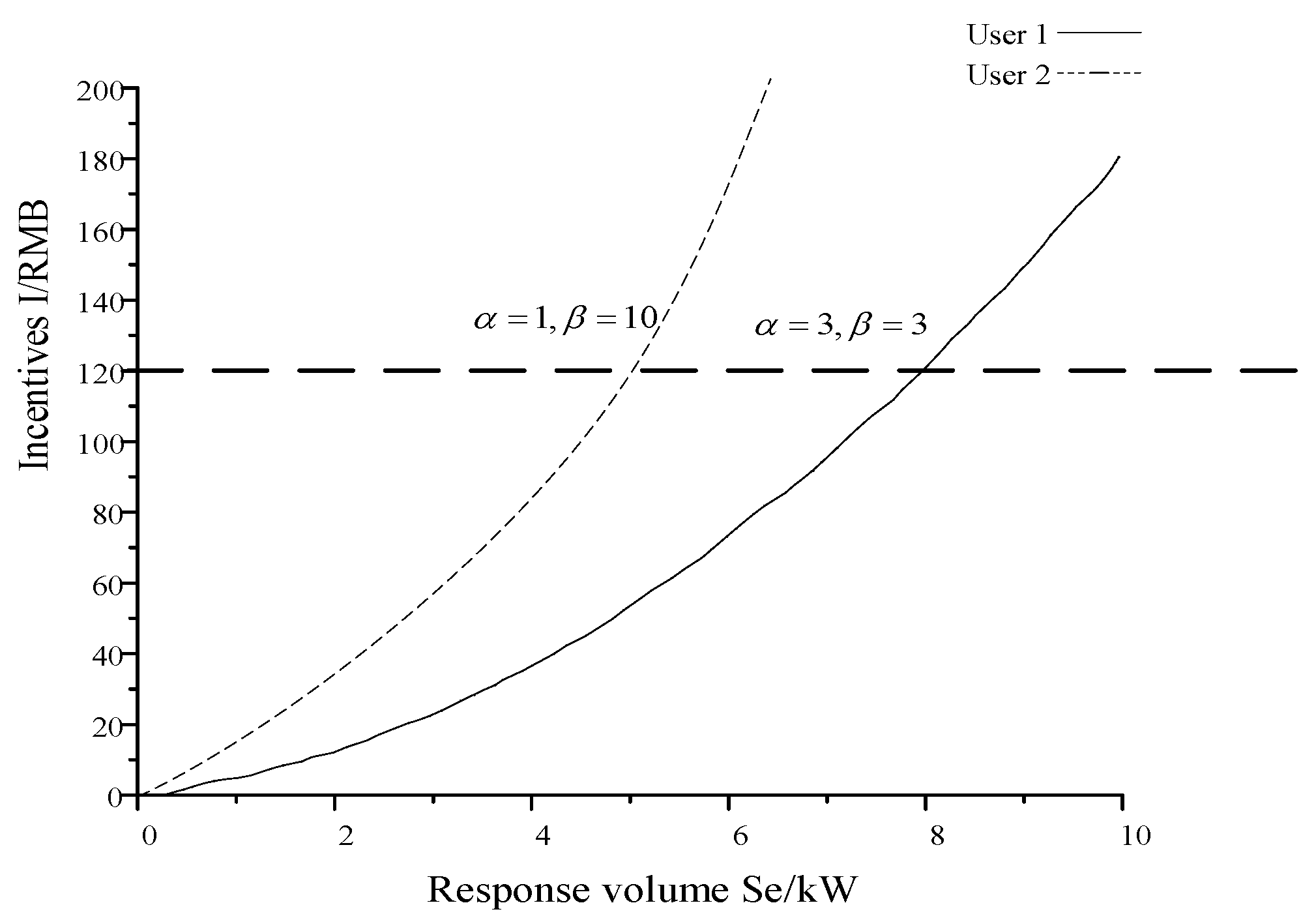
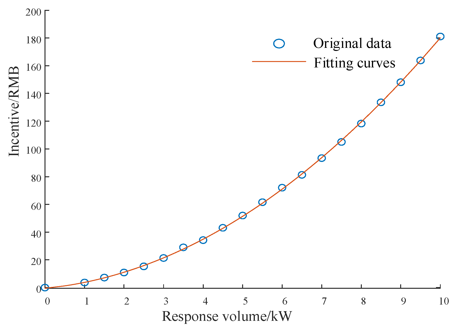
This paper fills a gap in the references by proposing an exogenous mode to consider random errors. The model obtains the demand-side response coefficient index of users in each case based on the identification and analysis of historical data. This index is used to build an exogenous model of demand-side response and incentive to characterize the demand-side response cost. It provides a clearer and more effective characterization of demand-side response costs and the relevance of traditional industrial pricing.

(b)

A strategy is proposed for the first time in this paper considering a two-stage master–slave game of user demand-side response. The first stage of the strategy is to form a time-of-day tariff for the day ahead and to regulate customers once. The second stage is an intraday correction of the tariff based on a model of the external characteristics of the customer’s demand-side response and the clean consumption incentive. Traditional pricing methods usually lack a specific consideration of user-demand response, and pricing strategies are too rigid to meet the flexibility needs of industrial users. Compared with traditional pricing methods, this innovative approach effectively meets the flexibility needs of industrial users and improves load regulation efficiency and cost-effectiveness. It improves the problem of traditional pricing strategies that failed to meet the flexibility needs of industrial users. The proposed pricing strategy is more economical and more effective in regulating the load.

(c)

This paper proposes introducing clean consumption subsidies and environmental cost factors into the incentive model. Through the adjustment of incentive indexes in various scenarios in the model, dynamic pricing is realized in the game to promote the consumption of renewable energy. This enables industrial park users to actively consume clean electricity and makes the effect of peak shaving and valley filling more significant. Traditional methods fail to adequately consider incentives for clean energy consumption. This leads to a low utilization rate for renewable energy. This paper incorporates clean consumption incentives and environmental cost factors into the incentive model. This encourages industrial park users to actively consume clean electricity, while enhancing the peak-and-valley regulation effect, further improving the effectiveness of load regulation.

The remainder of this paper is organized as follows. Section 2 builds an exogenous model of demand-side response and incentive to characterize the demand-side response cost. The method focuses more on describing the exogenous characteristics of user incentives and response quantities. Only the exogenous indicators and random errors in various typical scenarios need to be analyzed. The description of user demand-side response is more efficient. Section 3 presents a master–slave game dynamic pricing strategy that considers user demand response and is tailored to industrial parks. Section 4 analyzes a case study of industrial power users in a park in Liaoning. Finally, the paper is concluded in Section 5.

2. Industrial Power User Demand–Response Externality Model

2.1. Demand–Response Strategy for Industrial Parks

Industrial parks, as an important sector of local economic development, have a high demand for electricity and are more sensitive to electricity prices. Therefore, they tend to shift their loads based on electricity prices in order to reduce electricity costs without affecting production activities.

This paper uses demand-side response metrics to characterize the relationship between users, demand-side response volumes and costs. The external characteristics of industrial parks in various time periods and situations are modeled without analyzing the complex load composition inside users and building demand–response costs for various loads. Therefore, this model has the characteristics of high efficiency and clear characterization and reflects the allocation of demand-side resources. Through price incentives, a more efficient and flexible demand-side management can be established. The implementation framework of a demand–response strategy for industrial parks is shown in Figure 1.

2.2. Analysis of Demand–Response Characteristics of Industrial Park Users

2.2.1. Analysis of Demand–Response External Characteristics of Users

From the analysis, it is clear that the participation of users in regulation tasks in industrial parks is accompanied by certain losses. The size of the response of the launched user is proportional to the response cost.

$$S_{ei}\propto \frac{C_i}{S_{ei}}$$

(1)

As users increase the response volume, the cost of participating in demand-side response grows faster. The relationship is approximated as a quadratic functional relationship and is approximately expressed by the following Formula (2):

$$C(S_e)=\frac{1}{2}{\beta }_{\cos t}{S}_e^2+{\alpha }_{\cos t}{S}_e$$

(2)

where $S_e$ is the user’s response volume, $C(S_e)$ is the cost of participating in the demand-side response, and ${\alpha }_{\cos t}$ and ${\beta }_{\cos t}$ are the user’s demand-side response parameters. In general, the amount of response expected from a user is $S_e$, then the incentive given to user $I$ needs to be greater than or equal to its response cost. This means that users will spontaneously participate in a response only if the loss of participation is comparable to the reward received.

Considering the fluctuations and deviations in user behavior, as well as errors in the critical point due to constraints, there are two main sources of deviation in user incentives and responses: the first type of error comes from the variability of user behavior; the second type of error causes a deviation in the theoretical critical point. Taking into account the response error and constraints of users, Formula (1) is adjusted as follows:

$${\mathit{C}}_{re}(S_e)=\frac{1}{2}{\beta }_{re}{(S_e+\nu )}^2+{\alpha }_{re}(S_e+\nu )$$

(3)

$$s.t.\hspace{1em}\hspace{1em}{{\displaystyle }}^{}{S}_e\le L$$

where $C_{re}$ is the user’s response cost, $L$ is the user’s current load, $\nu$ is the user’s response error. ${\alpha }_{re}$ and ${\beta }_{re}$ are the user’s demand response parameters, and their values depend on the user’s response characteristics. As shown in Equation (4), the elasticity coefficient is related to the user’s demand response and incentive. Parameters ${\alpha }_{re}$ and ${\beta }_{re}$ are used as demand-side response indicators to characterize user demand-side response elasticity.

$$\epsilon =\frac{\mathrm{\Delta }{r}_b}{r_b}\frac{S_e}{\mathrm{\Delta }{S}_e}$$

(4)

In Formula (1), when the reward obtained by the user equals the loss incurred, the user’s objective is to participate in demand response with the lowest cost and maximum economic benefit. As the effect of lower order errors is relatively negligible, lower-order errors are omitted from the analysis of the user’s response elasticity. Substituting Formula (3) into Formula (4), the user’s response elasticity is obtained as follows:

$${{\displaystyle \mathit{\epsilon }}}_{S_e}=\frac{d{S}_e}{d{U}_{re}}·\frac{U_{re}}{S_e}=\frac{{\beta }_{re}{S}_e+2{\alpha }_{re}}{2{\beta }_{re}{S}_e+2{\alpha }_{re}}$$

(5)

where ${{\displaystyle \mathit{\epsilon }}}_{S_e}$ is the response elasticity of the user. Different users have different response elasticity, as shown in Figure 2.

From Formula (3), it is evident that parameters ${\alpha }_{re}$ and ${\beta }_{re}$ reflect the differences in the elasticity of demand response for different users. They describe the elasticity of the demand response on the demand side. Since the response elasticity of the same user varies at different times, users have different values of ${\alpha }_{re}$ and ${\beta }_{re}$ at different times of day. Identifying the demand response parameters during typical time periods suffices to obtain the demand response situation, as shown in Formula (6), for the load response.

$$S_{ei}^t=\sum _{i\in I}{S}_{eI}^t$$

(6)

$${\underset{¯}{S}}_{ei}^t\le S_{ei}^t\le {\overline{S}}_{ei}^t$$

(7)

The response behavior of users results in the loss of their own costs. As the degree of user participation in response increases, their losses increase at a faster rate. Therefore, a cost function for user participation in response is proposed as an approximation based on these characteristics:

$$C_i^t=\frac{1}{2}{\beta }_i^{}{(S_{ei}^t+{\nu }_i^t)}^2+{\alpha }_i^{}(S_{ei}^t+{\nu }_i^t)$$

(8)

where $C_i^t$ is the user’s response cost function. $S_{ei}^t$ is the response of user $i$ to the received stimulus in time period $t$. ${\alpha }_i^{}$ and ${\beta }_i^{}$ are the user’s demand-side response coefficients. The incentive factor is determined by fitting historical data for the user. In this model, once the demand-side response coefficient of the user for that time period is obtained, its response cost, which is the minimum incentive required, is obtained. The formation of this cost is no greater than the average electricity price in the market $q_{av}$, which gives rise to the following constraint:

$${\underset{¯}{C}}_i^t\le C_i^t\le q_{av}$$

(9)

2.2.2. Demand-Side Response Extrinsic Model Considering Random Errors

In Formula (8), due to the impact of external factors on users’ behavior, the error term ${\nu }_i^t$ is added. The uncertainty of response behavior leads to the error term ${\nu }_i^t$, which characterizes the noise caused by $i$ users in time period $t$. This deviation is result from temperature, weather, and typical day types. The error parameters formed by applying various indicators make the proposed model more accurate in characterizing users. These parameters are found in

Table 1. Factors considered in noise formation.

$\mathbf{Day}\mathbf{Type}$ (${\mathit{D}}_{\mathit{n}}$)	$\mathbf{Temperature}\mathbf{Data}$ (${\mathit{T}}_{\mathit{n}}$)	$\mathbf{Weather}\mathbf{Factor}$ (${\mathit{W}}_{\mathit{n}}$)	$\mathbf{Noise}$ (${\mathit{\nu }}_{}^{\mathit{t}}$)
Working day $D_1$	Temperature interval $T_1$	Type 1 $W_1$	${\nu }_i^t=(1+D_n{}^t\cdot T_n{}^t\cdot W_n{}^t){\nu }^t$
Holiday $D_2$	Temperature interval $T_2$	Type 2 $W_2$
Special Day $D_3$	Temperature interval $T_3$	Type 3 $W_3$
/	…	…
/	$T_n$	$W_n$

, which is formed referring to the fuzzy formula in reference [23] to enhance the objectivity and accuracy of the indicators. The input of the fuzzy controller is the error $e$ between the historical and current actual indicators and the rate of change in error $e_c$.

$$e_c=e(t)-e(t-1)$$

(10)

The output is the correction factor $\alpha \in [0,1]$ for the actual indicators, and the correction function is obtained as follows:

$$\mathrm{\Delta }=\alpha e-(1-\alpha )e_c$$

(11)

Based on the fuzzy formula, the following indicators are obtained:

$$\left\{\begin{array}{c}{D}_n{}^t=D^t+{\mathrm{\Delta }}_D\\ T_n{}^t=T^t+{\mathrm{\Delta }}_T\\ W_n{}^t=W^t+{\mathrm{\Delta }}_W\end{array}\right.$$

(12)

The specific indicators for demand-side response errors are listed in Table 1.

Therefore, the noise term ${\nu }_i^t$ is represented as:

$${\nu }_i^t=(1+D_n{}^t\cdot T_n{}^t\cdot W_n{}^t){\nu }^t$$

(13)

Moreover, since parameters ${\alpha }_i^{}$ and ${\beta }_i^{}$ are also affected by various environmental factors, they also need to be adjusted accordingly.

$$\left\{\begin{array}{c}{\alpha }_i^t=(1+D_n{}^t\cdot T_n{}^t\cdot W_n{}^t){\alpha }_i\\ {\beta }_i^t=(1+D_n{}^t\cdot T_n{}^t\cdot W_n{}^t){\beta }_i\end{array}\right.$$

(14)

The extrinsic model for user demand-side response and incentives is obtained as follows:

$$C_i^t=\frac{1}{2}{\beta }_i^t{(S_{ei}^t+{\nu }_i^t)}^2+{\alpha }_i^t(S_{ei}^t+{\nu }_i^t)+{\lambda }_i$$

(15)

where ${\lambda }_i$ is the error value due to other factors.

The total benefit of user demand-side response in time period $t$ is finally built as follows:

$$\begin{array}{c}{Y}_i^t=\left(I_0^t+{\gamma }^t\left(S_{ei}^t+{\epsilon }_i^t\right)\right)\cdot \left(S_{ei}^t+{\epsilon }_i^t\right)-C_i^t\\ \mathrm{s}.\mathrm{t}.0\le S_{ei}^t\le S_{ei-\max }^t\end{array}$$

(16)

where $Y_i^t$ is the user’s benefit, $I_0$ is the base incentive, $\gamma$ is the incentive at the given time. $S_{ei-\max }^t$ is the maximum response quantity of the user during time period $t$.

3. Dynamic Pricing Strategy Based on Master–Slave Game

3.1. Pricing Strategy Based on Master–Slave Game Theory

This paper proposes a dynamic pricing strategy for industrial parks based on master–slave game theory. The strategy aims to build a pricing mechanism for industrial parks under demand-side response incentives and environmental cost guidance that differ from the traditional master–slave game decision pricing. The proposed pricing strategy’s objective function to achieve dynamic pricing in different scenarios through a change in controllable quantities is the innovation of this chapter. The strategy consists of two stages: day-ahead and intra-day price adjustments. In the day-ahead stage, the power retailer develops electricity price information for each time period of the next day based on historical data, load forecasting, and daily load curves. The price includes the following components:

$${\zeta }_t={\chi }_t+{\chi }^u+{\chi }_t^p$$

(17)

where ${\chi }_t$ is the purchasing price of electricity, ${\chi }^u$ is the cost of using the distribution network, and ${\chi }_t^p$ is the profit obtained by the power retailer.

In the first stage, users adjust their electricity usage arrangements based on the day-ahead price information. The day-ahead tariff is corrected by controlling the intra-day incentive change. The second-stage objective function is built to maximize the revenue of electricity sellers and minimize the cost of electricity for customers. Price incentive constraints and park load characteristic constraints are set, and variable intra-day electricity sales prices are solved to achieve dynamic pricing. The process is illustrated in Figure 3.

When there is renewable energy access, to ensure the park users actively consume clean electricity, a clean consumption subsidy will be developed. The environmental cost factor is introduced on the basis of the traditional renewable energy consumption allowance. The carbon emissions of users are counted and an environmental cost factor is formed, and the renewable energy consumption allowance received by users is bounded by the environmental cost factor. This means customers consume renewable energy with lower carbon emissions.

For industrial power users, their environmental costs are calculated based on their “carbon footprint”. The original environmental cost calculation included industrial waste gas, wastewater, and solid waste. However, this strategy only considers the following two forms of pollution:

(a)

Industrial waste gas emissions

The pollution in the original industrial waste gas is calculated based on the emissions of sulfur dioxide and dust. To account for carbon emissions in decision-making, carbon dioxide emissions are also included in the calculation. The carbon footprint is calculated as follows:

$$p_q^I=\frac{c_1+c_2+c_3}{a_1}{r}_1$$

(18)

where $r_1$ is the balance factor of forestland in the area where the industrial park is located to absorb waste gas. $c_1$, $c_2$, and $c_3$ are the contents of sulfur dioxide, carbon dioxide and dust in the waste gas, respectively. $a_1$ is the absorption capacity of vegetation for sulfur dioxide, carbon dioxide, and dust.

(b)

Industrial wastewater emissions

The pollution in industrial wastewater is mainly calculated based on sulfur dioxide and chemical oxygen demand. Carbon emissions are also taken into account in the calculation. The carbon footprint is calculated as follows:

$$p_s^I=\frac{c_4+c_5+c_6}{a_2}{r}_2$$

(19)

where $r_2$ is the balance factor of wetlands in the area in which the industrial park is located for absorbing wastewater. $c_4$, $c_5$, and $c_6$ are the contents of sulfur dioxide, chemical oxygen demand, carbon in the wastewater, respectively. $a_2$ is the absorption capacity of wetlands for sulfur dioxide, chemical oxygen demand, and carbon.

3.1.1. Demand–Response Incentive

The demand–response incentive formulated by the electricity supplier needs to ensure the required response amount and minimize its own cost. Therefore, according to the analysis of user demand–response cost and incentive in Section 4. The demand–response cost for the electricity supplier is the minimum incentive required for user response in that time period. The incentive required for user $i$ in time period t is given by Formula (20). The formation of this model is based on the external characteristics of demand–response and incentives under different scenarios. The incentive varies with time and application scenarios.

$${\pi }_{ri}^t=\frac{1}{2}{\beta }_i^t{(S_{ei}^t+{\nu }_i^t)}^2+{\alpha }_i^t(S_{ei}^t+{\nu }_i^t)+{\lambda }_i^t$$

(20)

3.1.2. Incentive Model for Electricity Retailers

The incentive model of the power retailer is based on different scenarios, divided into two situations: with or without the integration of clean energy. Different incentives are set according to the response demand and the integration of clean energy. The incentive model for the power retailer when purchasing clean energy is as follows:

$${\pi }_e^t=(1-\sqrt{(\frac{P_i}{{\displaystyle \sum _{i=1}^n{P}_i}}{)}^2}){\pi }_e^t+\frac{1}{2}{\beta }_i^t{(S_{ei}^t+{\nu }_i^t)}^2+{\alpha }_i^t(S_{ei}^t+{\nu }_i^t)+{\lambda }_i^t$$

(21)

The incentive model for the power retailer when there is no clean energy access is:

$${\pi }_i^t=\frac{1}{2}{\beta }_i^t{(S_{ei}^t+{\nu }_i^t)}^2+{\alpha }_i^t(S_{ei}^t+{\nu }_i^t)+{\lambda }_i^t$$

(22)

3.2. Top-Level Revenue Function

3.2.1. Objective Function

The revenue objective function of the power retailer is:

$$W=\sum _t{q}_{t}L(t)-\omega \sum _t{q}_{\mathrm{c}}L(t)-(1-\omega )\sum _t{q}_{\mathrm{e}}(L(t))L(t)-f_C-{\pi }_i^t$$

(23)

$${\pi }_i^t=\left\{\begin{array}{c}(1-\sqrt{(\frac{P_n}{{\displaystyle \sum _{i=1}^n{P}_i}}{)}^2}){\pi }_e^t+\frac{1}{2}{\beta }_i^t{(S_{ei}^t+{\nu }_i^t)}^2+{\alpha }_i^t(S_{ei}^t+{\nu }_i^t),thereiscleanenergyaccess\\ \frac{1}{2}{\beta }_i^t{(S_{ei}^t+{\nu }_i^t)}^2+{\alpha }_i^t(S_{ei}^t+{\nu }_i^t),thereisnocleanenergyaccess\end{array}\right.$$

(24)

$$L(t)=L_1(t)-\mathsf{\Delta }L(t)$$

(25)

where $q_t$, $q_{\mathrm{c}}$, and $q_{\mathrm{e}}$ are the selling price, purchasing price, and clean energy price, respectively. ω is the proportion of clean energy purchases. $L(t)$ is the load at time $t$, ${\pi }_i^t$ is the cost of incentives for user response and clean energy consumption, which varies with different application times and scenarios as a controllable variable. $f_C$ is the risk cost of the electricity retailer. $L_1(t)$ is the electricity consumption before regulation at time $t$. $\mathsf{\Delta }L(t)$ is the electricity consumption adjusted for the load at time $t$.

Since the clean energy purchase cost in the revenue function of the power supplier is uncertain, the revenue function of the power supplier is also a random variable. Therefore, according to probability theory, the mean and standard deviation of the revenue function of the power supplier is obtained as follows:

$$\mu (W)=\sum _t{q}_{t}L(t)-\omega \sum _t{q}_{\mathrm{c}}L(t)-(1-\omega )\sum _t\mu (q_{\mathrm{e}}(L(t))L(t))-f_C-{\pi }_i^t$$

(26)

$$\delta (W)=\sqrt{{(1-\omega )}^2{\displaystyle \sum _t{\delta }^2(q_{\mathrm{e}}(L(t))L{(t)}^2}}$$

(27)

The upper-level model is built as shown in Formula (28):

$$\max \mu (W)-\delta (W)$$

(28)

3.2.2. Constraint Conditions

The constraints of the upper-level function are the upper and lower bounds of incentive prices. ${\pi }_t^{\min }$ is the minimum required incentive for user participation in demand–response at time $t$. ${\pi }_t^{\max }$ is the maximum required incentive for user participation in demand–response and the consumption of renewable energy, which is lower than the average electricity price level.

$${\pi }_t^{\min }\le {\pi }_i^t\le {\pi }_t^{\max }$$

(29)

For pricing, it is necessary to avoid the situation where the seller sets too high a price to ensure their profit. Therefore, the average dynamic electricity price of the seller needs to be within a certain limit. Its average value needs to be less than or equal to the market-average electricity price.

$$q_{\min }\le {\displaystyle \sum _t{q}_t}/24\le q_{av}$$

(30)

3.3. User Lower-Level Benefit Function

Objective Function

The objective function is to minimize the user’s electricity cost under the given conditions, where $Y_i^t$ is the benefit that user $i$ obtains from participating in demand-side response:

$$U_i^t=\min {\displaystyle \sum _t(q_t-Y_i^t-{\pi }_e^t})$$

(31)

The constraint for user participation in demand response is:

$$\sum _{t\in T_i}{\tau }_i^t=D{T}_i,\mathit{\forall }i\in \mathrm{I}$$

(32)

$$\sum _{t^{\prime }=t+1}^{t+C{T}_i}{\tau }_i^{t^{\prime }}\ge D{T}_i\cdot \left({\tau }_i^{t+1}-{\tau }_i^t\right),\mathit{\forall }i\in \mathrm{I},t\in \mathrm{T}$$

(33)

$$\prod _{t^{\prime }=t}^{t+C{T}_i}{k}_i^{t^{\prime }}=1,\mathrm{t}\in \left[1,96-D{T}_i\right]$$

(34)

where ${\tau }_i^t$ is the operating state of user $i$ at time $t$, with ${\tau }_i^t=1$ indicating that the user $i$ starts working at time $t$; otherwise, it stops working. $D{T}_i$ is the working cycle of user $i$, and $k_i^{t^{\prime }}$ are the response status of user $i$ at time $t$.

The power balance constraint is defined as:

$$L_t^{re}=\sum _{i\in I}{b}_i^r\cdot {\delta }_{t,i}$$

(35)

$$L_t=L_t^{base}+L_t^{re}$$

(36)

where $L_t^{base}$ and $L_t^{re}$ are the base load and the responsive load.

3.4. Game Theory Model for Power Retailers and Industrial Power Users

The proposed master–slave game model regards the power company as the leader and the users as the followers. Different incentive models are developed for different scenarios in the model, which is divided into two cases: with and without access to clean energy. Different incentives are formulated based on response demands and the use of clean energy, enabling dynamic pricing. Moreover, the incentive model includes clean energy consumption subsidies and environmental cost factors. It encourages users to reduce carbon emissions through the adoption of new production technologies and improved management. As followers, user electricity consumption behavior depends on their electricity cost model and usage limits.

$${\theta }_I=\left\{U_i^t,L_{i\min }^t\le L_i^t\le L_{i\max }^t\right\}$$

(37)

The power-seller’s decision set is determined by the user’s electricity consumption.

$${\theta }_s=\left\{W_I,\sum _{i=1}^I\sum _{t=1}^T{w}_i^t\left(L_i^t\right)=W_I,0\left.<w_i^t\left(L_i^t\right)<w_{s\max }\right\}\right.$$

(38)

where $L_i^t$ is the electricity consumption of user $i$ at time $t$, $w_i^t$ is the revenue of the sales company for the $i$-th user at time $t$. The objective functions are (29) and (30), respectively.

The master–slave game model is as follows:

$$\psi =\left\{I,{\left\{{\theta }_i\right\}}_{i\in I},\left\{{\theta }_s\right\},{\left\{U_i\right\}}_{i\in I},\left\{W_s\right\}\right\}$$

(39)

where I is the set of users and ${\theta }_i$ is the set of user decisions, namely electricity consumption. ${\theta }_s$ is the set of electricity seller decisions, namely electricity prices.

Assuming that the solutions for the upper- and lower-level models and their equilibrium solutions are a, b, and $a^{\ast }$, $b^{\ast }$, respectively, the game reaches equilibrium when the following conditions are met:

$$\left\{\begin{array}{l}{U}_i\left(a^{\ast },b^{\ast }\right)\ge U_i(a,b)\hfill \\ W_s\left(a^{\ast },b^{\ast }\right)\ge W_s(a,b)\hfill \\ \mathit{\forall }\alpha \in {\theta }_i\hfill \\ \mathit{\forall }\beta \in {\theta }_s\hfill \end{array}\right.$$

(40)

The specific game process is as follows: Firstly, the electricity seller, acting as the leader, sends rewards and demand responses to users, initiating the game. Secondly, users select the best countermeasures through the objective function. The electricity seller calculates the optimal price based on user responses and the objective function and sends this price back to users. Finally, this process is repeated until the final result is obtained, and the resulting electricity price is used to update the day-ahead price.

4. Case Study Analysis

In this paper, data for an industrial customer in a park in Liaoning province are selected. The demand-side response parameters are solved and modeled according to the load excitation–response curves of typical days under various scenarios of historical response data. The dynamic tariffs of two scenarios without and with clean electricity are calculated and analyzed.

4.1. Simulation Analysis of User Demand–Response Indicators

As shown in

Table 2. Historical user incentive–response data.

Incentive/RMB	Response/kW	Incentive/RMB	Response/kW
0	0	61.57	5.5
3.622	1	72.03	6
7.244	1.5	81.29	6.5
10.87	2	93.36	7
15.29	2.5	105.03	7.5
21.33	3	118.31	8
28.97	3.5	133.6	8.5
34.21	4	148.09	9
43.06	4.5	163.78	9.5
51.91	5	181.09	10

, historical load incentive–response consumption data provide a simplified exploration and understanding of the response characteristics of industrial loads under different scenarios. They are also effective for the construction of corresponding demand-side response models and dynamic tariff analysis.

Users actively participate in demand-side response when the incentive they receive is greater than or equal to their own cost of participating in demand-side response. Therefore, it is assumed that the incentive received by the load in the historical response data is its response cost. The analytical solution for the demand-side response index is shown in Figure 4.

The demand-side response indicator of user 1 for that time period is obtained by the data-fitting calculation ${\alpha }_1^t=2.70,{\beta }_1^t=3.08$. Therefore, the demand-side cost model of user 1 for that time period is obtained as:

$$C_1^t=1.54{(S_{ei}^t+{\nu }_i^t)}^2+2.70(S_{ei}^t+{\nu }_i^t)-0.28$$

(41)

By introducing a set of random noise simulations to the user response data, the modified demand-side response external characteristic model is expressed as:

$$C_1^t=1.528{(S_{ei}^t+0.032)}^2+2.62(S_{ei}^t+0.032)-0.28$$

(42)

The incentive results are shown in

Table 3. Calculation results of the proposed model.

Incentive/RMB	Response/kW	Incentive/RMB	Response/kW
0	0	65.33	5.696
4.866	1.105	75.407	6.176
9.013	1.697	84.872	6.599
12.439	2.098	96.306	7.08
18.391	2.689	109.01	7.582
23.578	3.133	124.42	8.155
30.826	3.683	135.37	8.54
36.752	4.087	154.11	9.165
43.54	4.512	171.04	9.698
54.69	5.147	182.9	10.057

. From Figure 3, it can be concluded that the average error of this model is only 8.1%, and it performs well in these applications.

Analysis and Comparison of Demand–Response Models under Two Scenarios

(a)

Scenario 1

As shown in

Table 4. Incentive and response consumption data in scenario 1 cases.

Time Point	Response Volume/kW	Incentive/RMB	Time Point	Response Volume/kW	Incentive/RMB
1	0.25	1	13	1.48	7
2	0.25	1	14	1.2	8
3	1.05	4	15	0.59	2
4	0.64	3	16	1.17	7
5	0.94	4	17	1.54	8
6	1.51	9	18	0.92	4
7	1.52	10	19	0.37	1
8	1.5	9	20	1.27	7
9	1.22	7	21	0.97	5
10	0.76	3	22	0.97	5
11	1.01	6	23	1.42	8
12	1.12	6	24	0.56	2

, presents the incentive and response consumption data in Scenario 1 cases.

In this scenario, the demand–response coefficient is ${\alpha }_{}^{t_1}=3.78,{\beta }_{}^{t_1}=2.96$. The results obtained when applying this parameter to build the model and performing analysis and calculation are shown in Figure 5.

(b)

Scenario 2

As shown in

Table 5. Incentive and response consumption data in scenario 2 cases.

Time Point	Response Volume/kW	Incentive/RMB	Time Point	Response Volume/kW	Incentive/RMB
1	0.37	1	13	1.58	7
2	0.37	1	14	1.69	8
3	1.12	4	15	0.67	2
4	0.78	3	16	1.23	7
5	1.03	4	17	1.62	8
6	1.64	9	18	1.03	4
7	1.71	10	19	0.49	1
8	1.68	9	20	1.36	7
9	1.42	7	21	0.99	5
10	0.87	3	22	0.99	5
11	1.18	6	23	1.6	8
12	1.21	6	24	0.61	2

,presents the incentive and response consumption data in Scenario 2 cases.

In this scenario, the demand–response coefficient is ${\alpha }_{}^{t_1}=3.56,{\beta }_{}^{t_1}=2.38$. Applying this parameter to build the model and performing analysis and calculation, the results are shown in Figure 6.

Through the above data analysis, the errors obtained under the two scenarios are shown in Figure 7. These errors perform well in calculations.

The traditional model does not take into account noise effects from various factors in user demand-side response, nor does it consider random errors from users. To compare the average model errors, 30 test points were chosen under the same scenario, considering and not considering random errors. The results are presented in Figure 8.

The results show that the average error of the model that considers noise factors is reduced. Therefore, the proposed model in this paper has a clearer and more efficient description of the load’s response to the user’s demand side. It is suitable for building demand-side response models for multiple types of users in industrial parks.

4.2. Analysis of Dynamic Electricity Prices under Two Scenarios

By analyzing the typical historical daily load incentive response volume curves for customers, the demand-side response volume can be obtained by the second stage of lower optimization. The required incentives are obtained as follows.

Table 6. Second-stage optimization response volume and required excitation.

Time Period	Actual Required Response/kW	Required Incentive/RMB
0:00–1:00	109.9	27.475
1:00–2:00	0	0
2:00–3:00	0	0
3:00–4:00	0	0
4:00–5:00	371.71	74.342
5:00–6:00	0	0
6:00–7:00	0	0
7:00–8:00	656.83	256.1637
8:00–9:00	1117.7	447.08
9:00–10:00	434.53	130.359
10:00–11:00	30	7.5
11:00–12:00	376.12	112.836
12:00–13:00	256.54	102.616
13:00–14:00	569.67	227.868
14:00–15:00	519.93	129.9825
15:00–16:00	432.46	172.984
16:00–17:00	418.1	83.62
17:00–18:00	71.03	14.206
18:00–19:00	0	0
19:00–20:00	81.07	16.214
20:00–21:00	139.19	20.8785
21:00–22:00	0	0
22:00–23:00	175.61	26.3415

shows the second-stage optimization response volume and required excitation.

It is possible to analyze the tariff in two scenarios: when there is renewable energy access and when there is no renewable energy access. The resulting two-stage dynamic tariff is as follows:

(a)

Scenario 1: No clean electricity

The load curve optimized by this strategy is shown in the Figure 9. As shown in Figure 9, through the two-stage electricity price guidance, the electricity seller can formulate prices that are closer to the needs of users and their own needs. As shown in Figure 10, the two-stage pricing strategy has a more significant effect on load transfer, peak shaving and valley filling.

(b)

Scenario 2: With clean energy integration

When clean energy (wind and solar power, for example) is integrated, the purchasing cost of the electricity seller decreases. Corresponding consumption subsidies are provided to users. The optimized electricity prices formed are as follows:

In this scenario, the load curve of the user is shown in Figure 11. This shows that after integrating clean energy, the purchasing cost of the electricity seller decreases and the user receives a clean consumption subsidy. Therefore, the user is more actively involved in the response and consumption of clean energy, resulting in a more significant effect of peak shaving and valley filling.

Analysis and Comparison of Dynamic Electricity Prices under Two Scenarios

The response of the load under the two-stage electricity price optimization strategy, with and without clean energy integration, was analyzed. As shown in Figure 12 and Figure 13, in the scenario with clean electricity access, due to the significant reduction in electricity costs for customers and the incentive of clean consumption subsidies, users are more actively involved in the response. This further strengthens the peak-shaving and valley-filling situation.

Table 7. Indicators under different optimization scenarios.

	Under the First Phase of the Tariff	Under Two-Stage Tariff (without Purchased Clean Electricity)	Under Two-Stage Tariff (Purchase of Clean Electricity)
Risk of electricity purchase/RMB	12,768.69	3884.3	2760
Clean electricity purchase risk/RMB	0	0	1962.3
Response cost/RMB	0	1904.71	1904.71
Clean consumption subsidy cost/RMB	0	0	1435.87
Profit of selling electricity/RMB	21,275.47	22,721.98	28,454.16
User cost/RMB	123,347.37	113,909.49	111,797.77
Peak-to-valley difference/MW	6.86	5.18	3.79

compares the economic benefits of the first-stage electricity price formation and the two-stage electricity price formation under the two scenarios.

As shown in Table 7, the two-stage optimization significantly reduces the purchasing risk cost for users and increases the demand response cost. After clean energy integration, the purchasing risk for clean energy increases, but the purchasing cost decreases. Compared to the scenario without clean energy integration, the profit of the electricity seller increases by 21.46% and the user cost decreases by 8.47% in this scenario. Furthermore, the peak-to-valley ratio under the two-stage electricity price is reduced by 24.5% compared to the first-stage electricity price. The peak-to-valley ratio under the scenario with clean energy integration is reduced by 26.83% compared to the scenario without clean energy integration. It can be seen that the two-stage electricity price-formation strategy has a more significant effect on peak-shaving and valley-filling. Therefore, the proposed pricing strategy is more economically efficient and more effective in terms of load control.

5. Conclusions

This paper proposes a demand–response-based master–slave game dynamic pricing strategy for industrial parks. The following conclusions are drawn from the simulation analysis:

(a)

A demand-side response externality model is built. It accurately describes the incentive response characteristics of industrial power users with an average error of about 17%, which is an 8.71% reduction compared to models without considering random errors.

(b)

The proposed model is efficient in describing demand-side response for various types of users in industrial parks. This approach offers a clearer representation of load and user demand-side response characteristics.

(c)

The proposed demand–response-based master–slave game dynamic pricing strategy for industrial parks shows enhanced economic efficiency. There is a 24.5% reduction in peak-to-peak difference using the two-stage tariff compared to traditional time-of-use pricing.

(d)

The load curve analysis reveals a 26.83% reduction in peak-to-peak difference when clean power is purchased. This indicates that clean power purchasing contributes to further peak-and-valley reductions, enhancing the effectiveness of the proposed pricing strategy for load regulation.

Future work is planned to take more error factors into account. The constraint relationship between the two will be further explored to bring the model closer to the displayed situation.

References

1. Heydarian-Forushani, E.; Golshan, M.E.H. Quantitative flexibility assessment of a comprehensive set of demand response programs. Int. J. Electr. Power Energy Syst. 2020, 116, 105562. [Google Scholar] [CrossRef]
2. Heydarian-Forushani, E.; Golshan, M.E.H.; Shafie-khah, M.; Catalão, J.P. A comprehensive linear model for demand response optimization problem. Energy 2020, 209, 118474. [Google Scholar] [CrossRef]
3. Sundaramoorthy, S.; Kamath, D.; Nimbalkar, S.; Price, C.; Wenning, T.; Cresko, J. Energy Efficiency as a Foundational Technology Pillar for Industrial Decarbonization. Sustainability 2023, 15, 9487. [Google Scholar] [CrossRef]
4. Hassan, M.A.S.; Chen, M.; Lin, H.; Ahmed, M.H.; Khan, M.Z.; Chughtai, G.R. Optimization Modeling for Dynamic Price Based Demand Response in Microgrids. J. Clean. Prod. 2019, 222, 231–241. [Google Scholar] [CrossRef]
5. Pietrasanta, A.M.; Shaaban, M.F.; Aguirre, P.A. Simulation and Optimization of Renewable Energy-Powered Desalination: A Bibliometric Analysis and Highlights of Recent Research. Sustainability 2023, 15, 9180. [Google Scholar] [CrossRef]
6. Jelić, M.; Batić, M.; Tomašević, N. Demand-Side Flexibility Impact on Prosumer Energy System Planning. Energies 2021, 14, 7076. [Google Scholar] [CrossRef]
7. Williams, S.; Short, M.; Crosbie, T.; Shadman-Pajouh, M. A Decentralized Informatics, Optimization, and Control Framework for Evolving Demand Response Services. Energies 2020, 13, 4191. [Google Scholar] [CrossRef]
8. Nassef, A.M.; Abdelkareem, M.A.; Maghrabie, H.M.; Baroutaji, A. Review of Metaheuristic Optimization Algorithms for Power Systems Problems. Sustainability 2023, 15, 9434. [Google Scholar] [CrossRef]
9. Long, Y.; Li, Y.; Wang, Y.; Cao, Y.; Jiang, L.; Zhou, Y.; Deng, Y.; Nakanishi, Y. Low-carbon economic dispatch considering integrated demand response and multistep carbon trading for multi-energy microgrid. Sci. Rep. 2022, 12, 6218. [Google Scholar] [CrossRef]
10. Mhanna, S.; Chapman, A.C.; Verbid, G. A Faithful and Tractable Distributed Mechanism for Residential Electricity Pricing. IEEE Trans. Power Syst. 2018, 33, 4238–4252. [Google Scholar] [CrossRef]
11. Al-Hajj, R.; Assi, A.; Neji, B.; Ghandour, R. Transfer Learning for Renewable Energy Systems: A Survey. Sustainability 2023, 15, 9131. [Google Scholar] [CrossRef]
12. Dadkhah, A.; Vahidi, B. On the network economic, technical and reliability characteristics improvement through demand-response implementation considering consumer 5 behaviour. IET Gener. Transm. Distrib. 2018, 12, 431–440. [Google Scholar] [CrossRef]
13. Tantau, A.; Puskás-Tompos, A.; Stanciu, C.; Fratila, L.; Curmei, C. Key Factors Which Contribute to the Participation of Consumers in Demand Response Programs and Enable the Proliferation of Renewable Energy Sources. Energies 2021, 14, 8273. [Google Scholar] [CrossRef]
14. Yang, H.; Zhang, J.; Qiu; Zhang, S.; Lai, M.; Dong, Z.Y. A Practical Pricing Approach to Smart Grid Demand Response Based on Load Classification. IEEE Trans. Smart Grid 2018, 9, 179–190. [Google Scholar] [CrossRef]
15. Yu, X.; Dong, Z.; Zheng, D. Research on Critical Peak Price Decision Optimization Considering Industrial Consumer’s Risk Appetite under the Carbon Neutrality Goal. Sustainability 2023, 15, 9347. [Google Scholar] [CrossRef]
16. Lei, W. The Optimal Decision Model of Peak-Valley Time-Sharing Tariff Based on User Response Mechanism and Its Impact Research; Hefei University of Technology: Hefei, China, 2020. [Google Scholar]
17. Karn, A.K.L.; Kakran, S. Operation Management of Microgrid Supplying to the Residential, Industrial and Commercial Community using Different Demand Response Techniques. In Proceedings of the 2022 4th International Conference on Energy, Power and Environment (ICEPE), Shillong, India, 29 April–1 May2022. [Google Scholar]
18. Zhou, C.; Ma, X.; Guo, X.; Lei, J. Interactive optimization operation method of integrated energy system in industrial park based on master-slave game. Power Syst. Autom. 2019, 43, 74–80. [Google Scholar]
19. Wang, H.; Li, K.; Zhang, C.; Ma, X. Distributed cooperative optimal operation strategy of community integrated energy system based on master-slave game. Chin. J. Electr. Eng. 2020, 40, 5435–5445. [Google Scholar]
20. Shandilya, S.; Szymanski, Z.; Shandilya, S.K.; Izonin, I.; Singh, K.K. Modeling and Comparative Analysis of Multi-Agent Cost Allocation Strategies Using Cooperative Game Theory for the Modern Electricity Market. Energies 2022, 15, 2352. [Google Scholar] [CrossRef]
21. Zhao, Y.; Xu, T.Q.; Li, Y.; Cui, L.; Chen, X. Research on electric vehicle scheduling strategy based on time-shared electricity price. Power Syst. Prot. Control. 2020, 48, 92–101. [Google Scholar]
22. Zhao, C.; Sun, J.; He, P.; Zhang, S.; Ji, Y. Integrating Risk Preferences into Game Analysis of Price-Making Retailers in Power Market. Energies 2023, 16, 3339. [Google Scholar] [CrossRef]
23. Zhu, W.; Luo, Y.; Hu, B.; Luo, H.; Zhang, Y.; Han, Y.; Tang, M.; Tong, Q. Thermal load elasticity and demand-side response of time-sharing tariff synergistically promote the optimal dispatch of electricity and heat for carbon emission reduction. Power Grid Technol. 2021, 45, 3803–3813. [Google Scholar]
Figure 1. The implementation framework of demand–response strategy for industrial parks.
Sustainability 15 12265 g001
Figure 2. User incentive–response curve.
Sustainability 15 12265 g002
Figure 3. Two-stage pricing strategy for power retailer and users.
Sustainability 15 12265 g003
Figure 4. User excitation–response volume fitting curve.
Sustainability 15 12265 g004
Figure 5. Calculation results of excitation under scenario 1.
Sustainability 15 12265 g005
Figure 6. Incentive calculation results under Scenario 2.
Sustainability 15 12265 g006
Figure 7. Error analysis under the two scenarios.
Sustainability 15 12265 g007
Figure 8. Comparison of model errors under the same scenario.
Sustainability 15 12265 g008
Figure 9. Electricity price of an industrial power user in a certain park without clean energy integration.
Sustainability 15 12265 g009
Figure 10. Load curve optimized by two-stage electricity price optimization.
Sustainability 15 12265 g010
Figure 11. Electricity price of an industrial power user in a certain park with clean energy integration.
Sustainability 15 12265 g011
Figure 12. Load curve after clean energy integration.
Sustainability 15 12265 g012
Figure 13. User response under the two scenarios.
Sustainability 15 12265 g013