Towards Cleaner Ports: Predictive Modeling of Sulfur Dioxide Shipping Emissions in Maritime Facilities Using Machine Learning

Abstract

Maritime ports play a pivotal role in fostering the growth of domestic and international trade and economies. As ports continue to expand in size and capacity, the impact of their operations on air quality and climate change becomes increasingly significant. While nearby regions may experience economic benefits, there are significant concerns regarding the emission of atmospheric pollutants, which have adverse effects on both human health and climate change. Predictive modeling of port emissions can serve as a valuable tool in identifying areas of concern, evaluating the effectiveness of emission reduction strategies, and promoting sustainable development within ports. The primary objective of this research is to utilize machine learning frameworks to estimate the emissions of SO₂ from ships during various port activities, including hoteling, maneuvering, and cruising. By employing these models, we aim to gain insights into the emission patterns and explore strategies to mitigate their impact. Through our analysis, we have identified the most effective models for estimating SO₂ emissions. The AutoML TPOT framework emerges as the top-performing model, followed by Non-Linear Regression with interaction effects. On the other hand, Linear Regression exhibited the lowest performance among the models evaluated. By employing these advanced machine learning techniques, we aim to contribute to the body of knowledge surrounding port emissions and foster sustainable practices within the maritime industry.

1. Introduction

Maritime activities for the transportation of goods have been identified as a significant source of air pollutants in coastal towns and river areas, with a substantial impact on regional air quality, climate change, and nearby communities’ exposure, thus contributing to health issues [1,2,3]. Air pollution is the fifth leading risk factor for mortality and the largest environmental health concern, causing one in every eight worldwide fatalities, or 7 million deaths each year [4]. Recent studies show that at least 70% of the emissions from ships on international routes occur within 400 km of the coast, where it has been concluded that ships in ports can contribute around 55 to 77% of total emissions in the areas close to the port [5,6,7,8]. However, these values depend on the city of study since, although its effect is significant, there is evidence that the impact of the land-based industry is much higher in cities with a high development in the mentioned activity [3]. As an illustration, the combined environmental costs associated with ships and trucks in the Port of Kaohsiung, Taiwan, are estimated to reach approximately $123 million annually [9].

With respect to the strategies proposed for the decrease in emissions, the use of fuels, such as liquefied natural gas (LNG), has been proposed, reaching a reduction in sulfur oxide (SOx) emissions by potentially 100% [10]. It should be added that this alternative is limited by the price of fuel, the volume of the container, the bunker fuel capacity of the ship and the carbon tax rate [11]. On the other hand, while scrubbers can manage to reduce SOx emissions, the overall problem with nitrogen oxide (NOx) emissions persists. Technologies such as “cold-ironing” have proven to be highly effective in significantly reducing hazardous emissions, including SOx, NOx, VOC, particulate matter (PM), CO, N2O, and CH4, in the local environment. Nevertheless, electricity powered by auxiliary engines (AE) is generally cheaper, and considerable capital investment must be made for these supply services. Despite this, in the long term there is an economic benefit if externalities are considered [7,10,12]. Consequently, since the last decade, although shipping has become more energy efficient, emission reduction still does not meet the standards of the International Maritime Organization (IMO), as the number of LNG carriers is increasing. The quantity of maritime emissions generated primarily depends on the operational mode of water-borne vessels, such as hoteling, maneuvers, and cruising, as well as the type of fuel utilized. It is worth noting that SO₂ emissions are predominantly influenced by the specific composition of the fuel employed rather than the type of engine used [13,14].

With the new opportunities that have arisen as a result of the current wave of digitization, terminal planning and management must be examined from a data-driven standpoint. Business analytics, as a valuable approach for extracting insights from operational data, plays a crucial role in mitigating uncertainty through forecasting and identifying the causes of inefficiencies, disruptions, and anomalies in both intra- and inter-organizational terminal operations. By leveraging business analytics, organizations can gain a better understanding of their operations, enabling them to address challenges and improve overall efficiency. Despite the increasing complexity of data within and surrounding container terminals, there is a dearth of data-driven initiatives in the container terminal setting [15]. However, few studies have investigated in-port emission prediction using machine learning and Deep Learning.

Consequently, our study seeks to obtain data that will help to address this research gap. The aim of this research is to utilize machine learning frameworks, including Linear Regression, Non-Linear Regression, and AutoML TPOT, to accurately estimate SO₂ emissions from ships during different port activities, such as hoteling, maneuvering, and cruising. By employing these advanced machine learning techniques, we seek to enhance our understanding of SO₂ emissions and contribute to the development of effective strategies for emission reduction in port environments.

We address the following research question: What is the most effective and accurate machine learning technique for predicting sulfur dioxide (SO₂) shipping emissions from maritime ports, and how can these predictions contribute to the development of sustainable environmental management strategies in the shipping industry?

To this end, our manuscript is organized as follows: Section 2 specifies the problem and puts it into perspective regarding the existing literature. Section 3 describes the problem under analysis. Section 4 explains the data sources, methods, and procedures. Section 5 provides details of the experiments undertaken as well as the related results. Section 6 includes some managerial insights, and Section 7 the conclusions.

2. Literature Review and Problem Statement

We first explore the topic of emission estimations. While nearby areas may experience economic benefits, there are significant concerns regarding air pollution, which has adverse effects on both human health and climate change. To address this problem, a port authority can create emission reduction programs and initiatives, the results of which can be tracked using an air emission inventory. Over the last two decades, there have been an increasing number of published studies of maritime emission estimation. Among these methods, the bottom-up approach has emerged as the most commonly utilized and is widely regarded by many authors as a more accurate and promising method for estimating emissions from maritime traffic [8,16,17]. In several of these studies, due to the unavailability of engine power data in the Automatic Identification System (AIS), default values were employed to estimate the maximum powers of main engines (ME), auxiliary engines (AE), and auxiliary boilers (AB) [5,12,16]. It is important to emphasize that the use of default values induces significant uncertainties in the calculation of emissions. However, in some cases when it is not possible to obtain specific information on loading factors, data from other studies are required [16]. Moreover, polluting ships may include tankers, general cargo ships, cruise ships, and container ships. Even when just the AE are operating, considerable emissions from the docking process may be found [18].

Most studies that estimated ship emissions in ports concluded that the majority were emitted during the hoteling stage [16,19,20], while maneuvering operations are identified as the least hazardous. The latter is due to the short duration of the maneuvering phase [12]. However, it varies from study to study indicating which of the other operation stages can become the most polluting [17,21,22,23], and it should be noted that this depends on type of vessels, the times and speeds for each phase, and the dimensions of the study area. For example, compared to cargo vessels, the energy demand (and emissions) of passenger vessels in ports is commonly higher due to a different type of operating patterns (a continuous use of the auxiliary engine at the dock) [12]. Despite this, due to the nature of most of the reported ports and the dimensions of the ports, it can be stated that in general, the container-type vessels were the ones that generated a higher level of emissions. Other studies showed that container vessels had higher fuel usage, whereas tanker vessels had higher ambient pollution levels in the berthing position, and that the primary discrepancies are related to the load factor parameter, the ME and AE power, and fuel consumption by vessel type [24].

Maritime ports are critical to the growth of both domestic and international trade and economy. Despite the previous concentration on emission inventory techniques, little research has been conducted on their implementation in information systems. Data confidentiality and ineffective information systems are important roadblocks that obstruct the generation of high-quality emission inventories and contribute to expenditures, thus appropriate information systems are needed to assist the establishment of high-quality emission inventories [25]. Information systems have become critical to ports’ competitiveness, improving communication and decision-making in order to improve visibility, efficiency, dependability, and security in port operations under a variety of scenarios [26]. As a result, it is required to conduct an academic and practical survey of contemporary information systems.

The sources of pollution include ships and logistics activities developed within the ports, such as the entry of trucks, and the use of cranes and forklifts [7]. Although the characterization of emissions is particularly difficult due to the multiple tasks carried out within the facilities, it is possible to develop pollution and control strategies to ensure the air quality of coastal cities using information obtained from inventories to analyze source contributions. Two approaches must be considered: (i) establishing an accurate inventory of ship emissions and (ii) quantifying the contribution of ship emissions [17]. Ship emission inventories can be classified into two primary methods: fuel-based (top-down) and activity-based (bottom-up) approaches. The fuel-based methodology relies on the combination of marine fuel sales data, encompassing quantities and types of fuel, along with fuel-related emission factors [24,27]. Several countries utilize the fuel-based approach (top-down) to develop national and international emission inventories. This approach is employed when accurate vessel traffic information is unavailable. However, it is recommended to prioritize the activity-based method as it offers more precise input parameters. The bottom-up approach, in contrast, necessitates comprehensive information on ship specifications, inspection and operational data, maximum speed, port calls, estimated shipping operations, and real-time operations [16]. This methodology is widely favored for estimating atmospheric emissions due to its utilization of more precise input parameters. It takes into account factors such as the time and power of the ME and AE, load factor (LF), maximum continuous rating (MCR), specific fuel consumption (SFC), emission factor for each engine in each navigation phase, and gross tonnage (GT) categorized by vessel type. Though, this method was found to be less accurate when elaborating on a regional scale [28]. Moreover, some suggested techniques include the PRISMA criteria. Through a multi-layer bottom-up study, an empirically organized foundation for the continued development of a unique indexing model of ship-gas emissions in port regions may be obtained [29].

Information obtained from these inventories serves as an input to several estimation models and tools such as C-FERST [30], EJSCREEN of the US Environmental Protection Agency (version 2016), C-line [31], and C-PORT [32], among others. Inputs to these models include emissions and meteorological information, and type of ships and vehicles, and in many cases new facilities, roads, or rail lines can be simulated, which can be added to create hypothetical scenarios, with the objective of planning sustainable development on a community scale. Also, there are other hybrid methodologies that consist of combining the different approaches of the aforementioned models [16]. More general settings of emission inventories are described in [25,33,34].

Further efforts should be made to obtain more accurate shipping emission estimations or inventories, so it is desirable to obtain more accurate input data (technical information on vessels, engines, load, and emission factors) to arrive at a global and universally accepted methodology [16,25,33,34]. Methodological approaches to learning inventory policies using machine learning could also be seen in [35] for a different application setting.

Second, we explore the Regulations. Maritime air pollution is widely recognized as a serious hazard to the health of coastal populations. As a result, several regulations to combat air pollution have been implemented across the world. Furthermore, policy and academic emphasis has shifted away from greenhouse gases, particularly CO₂, and toward other air pollutants. Historically, endeavors to mitigate the environmental consequences of international shipping emissions have not primarily prioritized addressing climate change concerns. Therefore, it has not been a topic of conversation in the different climate change conventions, added to the fact that significant portions of the emissions do not occur within the boundaries of any specific country.

The IMO, which is the formal regulatory body for the maritime sector, has adopted specific regulations to reduce air pollution [36] in specific areas around the world, called Emission Control Areas (ECA). The ECAs established so far are as follows: Baltic Sea Area, defined in MARPOL Annex I (SOx only); North Sea Area, defined in MARPOL Annex V (SOx only); North America Area, defined in MARPOL Annex VI Appendix VII (SOx, NOx, and PM); and finally, the US Caribbean Sea Area, defined in MARPOL Annex VI Appendix VII (SOx, NOx, and PM). Under the revised MARPOL Annex VI, the global sulfur limit was reduced to 0.50% (mass percent concentration) in 2020 [36].

As previously mentioned, one of the initiatives implemented by the IMO was the International Convention for the Prevention of Pollution from Ships (MARPOL). In 1997, MARPOL 73/78 introduced Annex VI, which specifically aimed at addressing air pollution from ships. Subsequently, in 2008, the IMO revised the regulations concerning the sulfur content of marine fuel, which are outlined in Annex VI of MARPOL. These changes were further updated in 2012 and implemented in Europe. As of 2015, vessels operating within SOx Emission Control Areas (SECAs) are prohibited from utilizing fuels with a sulfur content exceeding 0.5% by weight.

A highly relevant matter is how information systems have evolved to account for environmental concerns. Port Community Systems (PCSs) can have a significant impact on managing environmental pollution in ports. PCSs are electronic platforms that facilitate communication and collaboration among different stakeholders in a port, including shipping lines, terminal operators, customs officials, and trucking companies, which can improve environmental management practices. The authors of [37] provided a comprehensive review of the existing literature on PCSs, analyzing their findings and identifying gaps in the research. The authors also provided a classification scheme for PCSs based on their functionalities and examine the role of PCSs in enhancing port efficiency, sustainability, and resilience. Also, in [38], the authors explore the development of effective approaches for the implementation of PCSs and conduct a multivariate analysis of factors that affect the success of PCS implementation, such as the level of collaboration between stakeholders, the extent of data sharing, and the availability of technical infrastructure.

PCSs can help in managing environmental pollution by enabling the efficient monitoring and tracking of ships’ emissions, waste, and hazardous materials. PCSs can provide a platform for the exchange of data and information among stakeholders, allowing for better coordination and management of waste disposal and pollution control efforts. PCSs can also facilitate the implementation of environmental regulations, such as the IMO regulations on air pollution, which require ships to reduce their emissions of SOx and NOx in certain areas. PCSs can provide real-time data on ships’ emissions and compliance with regulations, allowing port authorities to take appropriate measures to address any violations. Moreover, PCSs can help in reducing the overall environmental impact of port operations by optimizing the use of resources and reducing energy consumption. PCSs can support the implementation of sustainable practices, such as the use of renewable energy and the promotion of eco-friendly transportation modes. PCSs can play a vital role in managing environmental pollution in ports by enabling better communication, collaboration, and coordination among stakeholders, facilitating compliance with regulations, and promoting sustainable practices.

Last, in the field of environmental sciences, machine learning (ML) methods have been widely used with a high success rate. The authors in [39,40] present innovative research on the application of hybrid wavelet-ML models in the domain of environmental science and hydrology. [41] presents a comprehensive review of the challenges in modeling, optimization, diagnostics, and control of Internal Combustion Engines (ICE); and explores the potential of modern ML techniques, proposing a ML-based grey-box approach as a robust solution to address these challenges for ICEs. The authors of [42] used Deep Learning for effectively predicting CO₂ emissions, with a case study in India. The authors of [43] provided a review of ML algorithms in air quality modeling. An interesting approach is presented in [44] for the prediction of SO₂ pollutants with a case study in Portugal. The study applies Bayesian, econometrics, and ML models to predict SO₂ emissions in Portugal and concludes that ML models exhibit better generalization power compared to classical approaches.

3. Problem Description

Presently, the global port industry confronts numerous challenges that encompass accommodating increasingly larger ships; contending with emerging ports; addressing transportation bottlenecks in the movement of goods, raw materials, and people between land and sea; and, more recently, addressing environmental concerns associated with air, land, and water pollution stemming from ships. Moreover, these challenges manifest within a commercial context that necessitates the industry to sustain viability, competitiveness, and profitability [45].

While shipping is the most environmentally friendly mode of transportation in terms of emissions/fuel consumption per ton of cargo [46], it contributes significantly to air pollution. About 90% of the goods worldwide are transported by maritime means [5,8], of which it is estimated to contribute approximately 2.4% of global greenhouse gas emissions derived from anthropogenic sources. The emission of atmospheric pollutants resulting from port operations poses a significant threat to the ecological equilibrium of nature and urban environments. Additionally, it has adverse consequences on global climate change and human health, further amplifying the risks associated with port activities [8,11,47,48]. Its share is expected to increase in the future, so these emissions will remain a major burden for the long term, especially for coastal cities with large ports [28,49]. Specifically, for air pollutants, estimates show that ships release 1.2 to 1.6 million tons of PM₁₀, 4.7 to 6.5 million tons of SOx, and 5 to 6.9 million tons of NOx worldwide [8,16]. From this, it has been determined that the highest costs associated with externalities occur at the local level [3].

In contrast to the increasingly stringent emission control of road vehicles, policies and regulations for the prevention and control of ship emissions remain insufficient and ineffective; thus, many port authorities continue to ignore the importance of sustainable development [28,46]. Studies conducted in Latin America show that current environmental regulations will include the use of fossil fuels, particularly marine fuels, like marine diesel oil, in port systems for some time [24].

Developing an effective regulatory framework to enhance air quality necessitates obtaining more precise information regarding the sources and contributors of emissions. This entails not only accurately calculating emissions through comprehensive data on vessel movements, including position, speed, technical configuration, and operational characteristics, but also addressing the disaggregation of results by vessel categories and subcategories [10]. Such detailed insights are crucial for devising targeted strategies and measures to mitigate emissions and improve air quality within the maritime industry. Ports are going to face considerably more pressure in their efforts to cut emissions as a result of the present societal and political trends. Port authorities may create and follow the progress of effective emission-reduction strategies by monitoring and reporting emissions analyzed with emission inventories. A possible aspect is to include optimization models, ML, and gamification via collaboration among port stakeholders to share important data and employ appropriate visualization approaches [50].

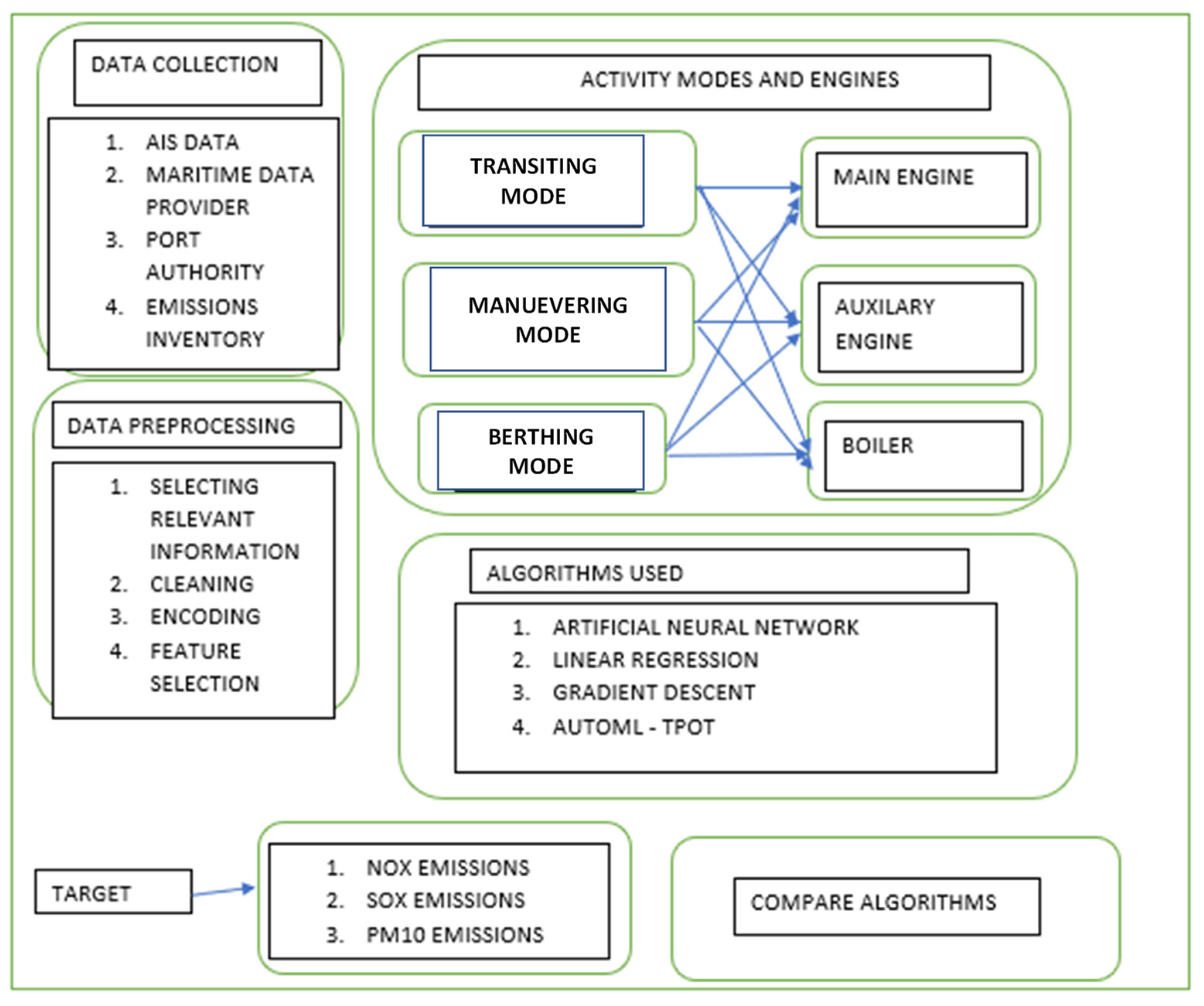
4. Data Sources, Methods, and Procedures

4.1. Data Sources

The given analysis was conducted for the Port of Barranquilla, Columbia. The dataset used for this analysis was obtained from DIMAR (General Directorate of Maritime), which is a Colombian authority in charge of organizing, coordinating, and controlling maritime operations in the country. The data was obtained for the year 2018. DIMAR provided the inventory information of the vessels that docked at the Barranquilla port and the type of ship carrier. The details regarding the technical information of the vessels were obtained from the Automatic Identification System (AIS), also known as AIS marine traffic. The details, such as year of construction, gross tonnage, and average and maximum speed, were obtained from this database.

The internal combustion processes in ships’ engines, both main and auxiliary, give rise to approximately 450 different pollutant species that have an impact on air quality. These emissions occur during various ship activities, including sailing, maneuvering in and out of the port, as well as when ships remain docked. Among these pollutants, PM, NOx, SO₂, CO, CO₂, hydrocarbons (HC), and volatile organic compounds (VOCs) are of particular significance due to their adverse effects on both human health and the environment. In our analysis, we have specifically developed a model to estimate SO₂ emissions, recognizing its importance as one of the key pollutants.

The data obtained from the above-mentioned data sources was further re-modeled by [51] and has been used in our analysis. After agglomerating the above-mentioned data sources, the combined data set had a multitude of features, as indicated in

Table 1. List of the variables in the dataset.

Variable Type	Description
Motor ship	Type of motor ship
Type of load	Type of load
Docking day	Date on which the ship docked into the port
Docking time	Docking Time
Sailing day	Date on which the ship sailed from the port
Departure time	Time at which the ship departed from the port
Permanence	Duration of stay of the ship at the port
Year of construction	The year in which the motor ship was constructed
Max speed	Max speed of the ship
Average speed	Average speed of the ship
Gross Tonnage	Gross tonnage of the ship
Dead weight	Dead weight of the ship
ME fuel	Main engine fuel type
AE Fuel	Auxiliary engine fuel type
Engine speed	Speed of the engine
Power-ME (kW)	Power used by the main engine
LF ME Cruising	Load factor for the main engine during cruising
A ME	Technical factor for the main engine
Power-AE (kW)	Power used by the auxiliary engine
LF ME Maneuver	Load factor for the main engine during maneuver
Energy-ME Cruising	Energy used by the main engine during cruising
Energy-ME Maneuver	Energy used by the main engine during maneuver
Energy-AE Cruising	Energy used by the auxiliary engine during cruising
Energy-AE Maneuver	Energy used by the auxiliary engine during maneuver
Energy-AE Hotelling	Energy used by the auxiliary engine during hoteling
ME Cruising	Emissions by the main engine during cruising
ME Maneuver	Emissions by the main engine during maneuver
AE Cruising	Emissions by the auxiliary engine during cruising
AE Maneuver	Emissions by the auxiliary engine during maneuver
AE Hotelling	Emissions by the auxiliary engine during hoteling
Caldera Hotelling	Emissions by the boiler during hoteling
Subtotal (NoCald)	Total without boilers
Total	Total including boilers

.

The objective of the research was not to replicate what had been proposed in [51] using ML, but rather to examine if we can accurately predict SO₂ emissions by making use of a combination of top-down (fuel-based) and bottom-up (activity-based) estimation approaches. We performed some data preprocessing and feature selection procedures before moving forward with the analysis. The original dataset from [51] was in the form of a report. Hence, we had to perform a pivot operation on the data to bring it into a tabular format which can be used for analysis (see Figure 1 and Figure 2,

Table 2. Original data before transformation (an excerpt).

Motor Vessel	Load Type	Docking Day (DD/MM/YYYY)	Docking Hour	Departure Day (DD/MM/YYYY)	Departure Hour	Total Hours	Construction Year	IMO
CAP PORTLAND	Container	1/01/2018	22:10:00	2/01/2018	4:50:00	6:40:00	2007	9,344,631
HANSA AUGSBURG	Container	2/01/2018	16:10:00	3/01/2018	1:00:00	8:50:00	2008	9,373,474
HOHEBANK	Container	3/01/2018	9:45:00	3/01/2018	15:10:00	5:25:00	2007	9,435,818
ULTRA CORY	Bulk	1/01/2018	11:40:00	5/01/2018	18:25:00	102:45:00	2014	9,675,743
MAERSK WAKAMATSU	Container	5/01/2018	14:00:00	6/01/2018	0:05:00	10:05:00	2010	9,550,345
YERUPAJA	Container	5/01/2018	19:40:00	6/01/2018	13:00:00	17:20:00	2010	9,412,488
MAERSK WALVIS BAY	Container	6/01/2018	22:45:00	7/01/2018	15:25:00	16:40:00	2010	9,550,369
HOHEBANK	Container	7/01/2018	11:55:00	7/01/2018	19:15:00	7:20:00	2007	9,435,818
SAN ADRIANO	Container	8/01/2018	21:40:00	9/01/2018	7:40:00	10:00:00	2008	9,347,279

).

The importance of individual features in predicting SO₂ emissions is essential for understanding the driving factors behind pollution levels and devising effective emission reduction strategies. Feature important analysis helps identify the most influential variables that significantly contribute to the variation in SO₂ emissions. Through feature importance analysis, we can ascertain which specific variables have the most substantial influence on SO₂ emissions. These factors include Fuel Type and Quality, Vessel Type and Size, Engine Specifications, and Vessel Activity. The implementation of emission-reduction policies and practices by port authorities and shipping companies, which can influence the emission levels within the port area, were not addressed in this study. Moreover, continuous monitoring and analysis of feature importance can help track the effectiveness of the implemented measures over time.

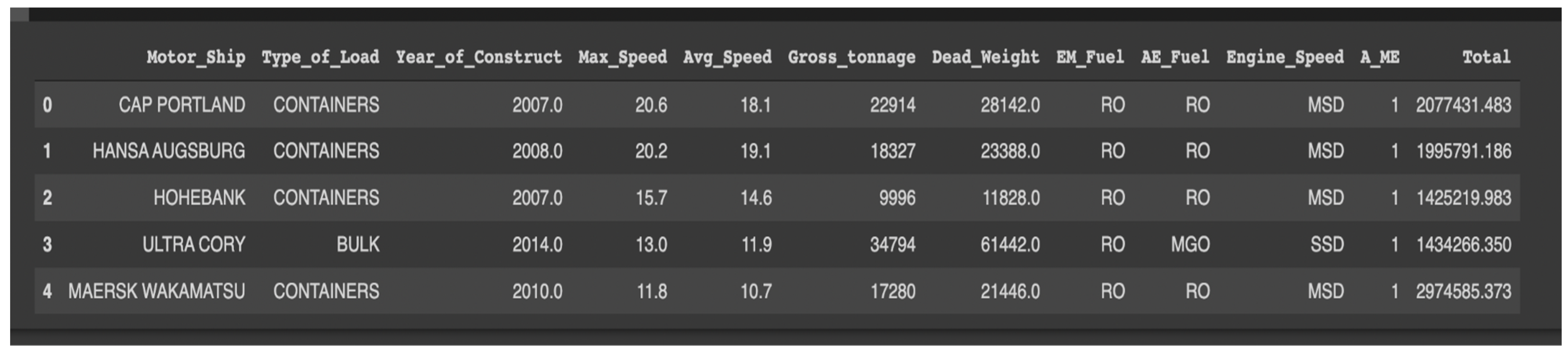
4.2. Exploratory Data Analysis and Pre-Processing

In order to better understand the data and the predictors, we conducted some basic exploratory data analysis. The objective of this task was to understand the spread of the data and the data types to check for missing data. Categorical variables within our data were encoded as numbers before fitting them to the model. We used label encoder to encode categorical variables as the number of unique values for each categorical variable was high. Figure 2 shows how our data types would look if we had chosen to use One Hot Encoder, which splits the categorical into n − 1 unique columns.

4.3. Model Selection

As our outcome variable, Total Emissions, is a continuous variable, our problem is a regression problem. In order to predict the total emission value, we explored several ML models, such as Multiple Linear Regression, Multiple Non-Linear Regression, and AutoML TPOT Regressor.

4.4. Multiple Linear Regression

Linear Regression serves as one of the basic ML models employed for regression tasks, specifically for predicting continuous variables. Multiple Linear Regression, on the other hand, is a statistical technique utilized to forecast the outcome of a variable based on two or more variables’ values. Multiple regression extends the concept of Linear Regression by incorporating multiple independent or explanatory variables while the dependent variable represents the variable we aim to predict. The independent variables are used to anticipate the value of the dependent variable.

Multiple regression can be represented by the following formula:

ŷ = b₀ + b₁X₁ + b₂X₂

(1)

where

ŷ is the predicted value of a dependent variable;

X₁ and X₂ are independent variables;

b₀, b₁, and b₂ are regression coefficients.

4.5. Multiple Linear Regression with Interaction Effects

The Linear Regression model operates under the assumption of a consistent linear relationship between the predictors and response variables. However, this assumption may not always hold true. In certain cases, an interaction effect emerges in regression, whereby the impact of one independent variable on another is dependent on the value(s) of one or more additional independent variables. Consequently, the regression equation incorporating an interaction effect would be as follows:

Ŷ = b₀ + b₁X₁ + b₂X₂ + b₃X₁X₂

(2)

In this equation (Equation (2)), the coefficient b₃ represents the regression coefficient, and X₁X₂ represents the interaction term. Specifically, the interaction between X₁ and X₂ is referred to as a two-way interaction since it involves the interplay between two independent variables.

4.6. AutoML TPOT Regressor

Automated Machine Learning (AutoML) is a term used to describe strategies that automate the process of identifying high-performing models for predictive modeling tasks with very low human intervention. One notable Python-based open source library for AutoML is TPOT. TPOT combines the popular Scikit-Learn ML package, which includes data transformations and ML algorithms, with a genetic programming stochastic global search technique. This combination enables TPOT to efficiently discover the model pipeline for a given dataset. TPOT represents a model pipeline as a tree-based structure, incorporating data preparation, modeling techniques, and model hyperparameters. Through an optimization process, TPOT identifies the most suitable tree structure for a specific dataset. The genetic programming approach enables TPOT to conduct stochastic global optimization by representing programs as trees. TPOTRegressor specifically focuses on supervised regression models, preprocessors, feature selection techniques, and any other estimator or transformer that adheres to the Scikit-learn API. Additionally, TPOTRegressor explores various hyperparameters within the pipeline. For a visual representation of TPOT’s architecture and its links to the used methodology, refer to Figure 3, which provides a concise overview.

By default, TPOTRegressor performs an extensive search encompassing a diverse range of supervised regression models, transformers, and hyperparameters. However, it is worth noting that the behavior of TPOTRegressor can be completely customized using the config_dict parameter. This allows for precise control over the models, transformers, and specific parameters that TPOTRegressor explores during its search process.

Table 3. Hyperparameters of TPOT.

Parameters	Description
generations	This parameter dictates the number of iterations to the run pipeline optimization process.
population_size	This parameter specifies the number of individuals to be retained in the genetic programming population in each generation.
mutation_rate	In the range [0.0, 1.0], this parameter tells the GP algorithm how many pipelines to apply random changes to every generation (“Using TPOT—Epistasis Lab”).
crossover_rate	The range for this parameter is set from 0.0 to 1.0, and it determines the number of pipelines that the genetic programming algorithm will “breed” in each generation (“TPOT API—Epistasis Lab”).

provides some of the important hyperparameters of TPOT. The reader is directed to the appendix for further clarity of TPOT parameter tuning.

4.7. Model Building

We used Python and its ML Libraries, such as Scikit-learn and keras, for building models for Linear Regression, Linear Regression with interaction effects, and AutoML TPOT regression. For our analysis, we split the dataset into two parts, training data and testing data with a ratio of 70:30 (“Generalization and evaluation|Machine Learning in Java—Second Edition”). The model was built and trained on the 70% of the training dataset and was tested against the remaining 30% of the test dataset.

4.8. Model Evaluation

Once the model was built, it was tested on the training dataset. Model evaluation or assessment is the process of analyzing a ML model’s performance, as well as its strengths and limitations, using various evaluation criteria. Model evaluation is critical for determining a model’s efficacy during the early stages of research, as well as for model monitoring. We have used the following evaluation metrics for assessing the model’s performance:

(1)

Explained Variance Score;

(2)

Mean Absolute Error;

(3)

Mean Squared Error;

(4)

R Squared.

4.8.1. Expanded Variance Score

If ŷ is the estimated target output, y the corresponding (correct) target output, and Var is “Variance, the square of the standard deviation, then the explained variance is estimated as” (“Explained Variance Regression Score—GM-RKB—Gabor Melli”) follows:

$$explained variance\left(y,\widehat{y}\right)=1-\frac{Var\left(y-\widehat{y}\right)}{Var\left(y\right)}$$

(3)

4.8.2. Mean Absolute Error (MAE)

The degree of mistake in your measurements is known as absolute error. It is the distinction between what was measured and what was “true”. If a scale reads 90 pounds but you know your exact weight is 89 pounds, the instrument’s absolute inaccuracy is 90 pounds − 89 pounds = 1 pound.

$$MAE=\frac{{{\displaystyle \sum }}_{i=1}^n\left|y_i-x_i\right|}{n}$$

(4)

4.8.3. Mean Squared Error (MSE)

A Mean Squared Error (MSE) indicates how near it is to a set of points. It accomplishes this by squaring the distances between the actual points and the predicted points. Squaring is required to eliminate any negative signals. It also gives significant discrepancies more weight. Because one is calculating the average of a series of mistakes, it is termed the Mean Squared Error. The lower the MSE, the better the forecast.

$$MSE=\frac{1}{n}{\displaystyle \sum }_{i=1}^n{\left(Y_i-{\widehat{Y}}_i\right)}^2$$

(5)

4.8.4. R Squared

R-squared (R²) is a statistical metric that quantifies the amount of variation explained by an independent variable or variables in a regression model for a dependent variable.

$$R^2=1-\frac{RSS}{TSS}$$

(6)

where,

• RSS—the sum of squares of residuals, or Unexplained Variation;
• TSS—the total sum of squares, or Total Variation.

5. Experiments and Results

Each of the models was trained and tested on combinations of hyperparameters to find the models that could best fit the data in both training and testing environments. The goal was to find a model that would yield the best R² value and the lowest MAE/MSE values without overfitting the data.

Table 4. Hyperparameter experimentation on TPOT Regressor.

Model	Generation	Population Size	Explained Variance Score	Mean Absolute Error	Mean Squared Error	R Squared
TPOT	5	20	0.917	263,076.438	169,158,704,289.928	0.917
TPOT	10	20	0.993	81,184.105	15,300,590,965.080	0.992
TPOT	15	20	0.972	118,898.773	56,674,543,758.253	0.972
TPOT	20	20	0.973	147,333.593	55,117,989,894.453	0.973
TPOT	5	40	0.986	97,174.019	28,898,605,308.472	0.986
TPOT	10	40	0.956	148,109.881	89,142,008,587.043	0.956
TPOT	15	40	0.958	120,343.064	85,122,331,552.718	0.958
TPOT	20	40	0.976	110,162.189	47,905,723,160.474	0.976

provides a summary of some of the experiments conducted on the TPOT Regressor model. From the table, we can see that the TPOT model with generation = 10 and population_size = 20 (indicated in bold) yields the best R² value and the lowest MAE value. Ideally, this model should be considered as the best model as it gives the best results. However, this might not always be true. Such a high R² value might indicate that our model is overfitting the data and we, therefore, need to introduce some variance during the training phase. However, a model with generation = 20 and population_size = 40 (also indicated in bold) yields the second-best results in terms of R² and MAE and has a slightly lower R² and, therefore, might be a good candidate for the final model.

From

Table 5. Results of Linear and Non-Linear Regression.

Name	Predictors	Interactions	Explained Variance Score	Mean Absolute Error	Mean Squared Error	R Squared
Multiple Linear Regression	11	No	0.916	244,065.10	170,566,648,568.52	0.916
Multiple Non-Linear Regression	7	No	0.900	254,623.72	202,454,660,520.95	0.900
Multiple Non-Linear Regression (with interaction effects)	10	Yes	0.957	207,464.72	87,093,043,507.19	0.957

, we can see that the Non-Linear Model with interaction effects gives us the best results on the test dataset, although it still lags when compared to the best Auto-ML TPOT models fitted.

The interpretability of ML models is a critical aspect in the context of predicting SO₂ emissions in maritime ports. Stakeholders, including port authorities, policymakers, and environmentalists, need to understand the factors influencing the predictions to make informed decisions and devise effective emission-reduction strategies. Let us discuss the interpretability of the ML models used in this analysis, namely AutoML TPOT, multiple regression, and multiple regression with interactions.

AutoML TPOT is an automated ML tool that uses genetic programming to identify the best model pipeline for a given dataset. While AutoML TPOT is powerful and efficient in finding complex model architectures and hyperparameters, its interpretability can be a challenge. The resulting model pipeline may be composed of various transformations and algorithms, making it difficult to interpret the exact relationship between features and predictions. Also, the black-box nature of AutoML TPOT may hinder the ability to gain insights into the driving factors of SO₂ emissions. Supplementary Materials shows the python code for all the models ran for prediction of pollutants.

5.1. Running the Model on Unseen Data

To assess the performance and generalizability of our ML models for predicting SO₂ shipping emissions from maritime ports, we conducted experiments using unseen data. This data consisted of a separate set of observations that were not included in the training or validation stages of the model development process. In addition, we added noise to the observed data to add randomness to the set to make the results more generalizable.

Upon evaluating the models with this unseen data, we observed encouraging results. The predictions of SO₂ emissions from shipping activities demonstrated strong accuracy and reliability. The models successfully captured the underlying patterns and relationships between the input features and the emission levels, allowing for accurate estimation.

Specifically, our ML models achieved a high level of precision in predicting SO₂ emissions for unseen data, with minimal deviation from the actual emission measurements. The models showcased their ability to generalize well beyond the training dataset, indicating their robustness in handling new and unseen data instances.

Furthermore, we conducted comparative analyses with existing prediction models and reference datasets. The results demonstrated that our ML-based approach outperformed traditional methods and exhibited superior predictive capabilities for SO₂ shipping emissions. This suggests the potential of ML as an effective tool for accurate and efficient estimation of emissions in maritime ports.

Table 6. Results on unseen datasets.

Name	Generations/Predictors	Population Size/Interactions	Expanded Variance Score	Mean Squared Error	R Squared
TPOT	10	No	0.9205	130,258,340,925.97	0.919
Multiple Non-Linear Regression (with interaction effects)	10	Yes	0.9134	140,897,779,956.84	0.912

shows the results for unseen data for the best TPOT and regression (with interactions) models. Results are similar for each one of the best TPOT and regression models, with a better performance for the best TPOT structure. These results not only validate the efficacy of our developed models, but also highlight their potential practical applications. The accurate prediction of SO₂ shipping emissions using machine learning can support decision-making processes, facilitate the implementation of targeted emission-reduction strategies, and contribute to the development of sustainable environmental management practices in the shipping industry.

It is worth noting that while the results for unseen data are promising, ongoing monitoring and further validation efforts will be essential to ensure the continued accuracy and reliability of the prediction models. Continued data collection and integration of real-time monitoring systems will enable constant updates and refinements to the models, leading to improved predictions and enhanced sustainability in maritime port operations.

The results obtained for unseen data reaffirm the effectiveness of our ML models in predicting SO₂ shipping emissions from maritime ports. These results hold great promise for their practical application in environmental management and decision making, ultimately fostering sustainable practices and reducing the environmental impact of shipping activities.

5.2. Limitations or Bias in the Datasets

As with any data-driven research, it is crucial to acknowledge potential limitations, biases, inaccuracies, and data gaps that might influence the reliability and generalizability of the findings. When analyzing data for predicting pollution in maritime ports, the following considerations should be taken into account:

• ▪ The reliability of the predictions heavily relies on the quality and completeness of the data collected. Inaccurate or incomplete data, such as missing values or errors in recording, can introduce biases and reduce the accuracy of the models.
• ▪ Data outliers or anomalies can distort the analysis, leading to misleading predictions. Identifying and appropriately handling these anomalies is crucial to ensure the accuracy of the results.
• ▪ In some cases, historical data might be limited or not available, especially for emerging ports or new operations. This limitation can affect the model’s ability to capture long-term trends and make accurate forecasts.
• ▪ Changes in operating conditions, such as the introduction of new technologies or shifts in vessel types, can impact the relevance of historical data for predicting future emissions.

To address these limitations and biases, we have performed data-cleansing techniques and added noise to the unseen dataset analyses for increased randomness to test the quality of the predictors. Ensuring transparency in the data collection process and detailing potential limitations in the research findings enhances the credibility of the predictions and supports well-informed decision making. Additionally, the continuous monitoring and validation of predictive models can help maintain their accuracy and reliability over time.

5.3. Lessons Learned

Some of the lessons learned are summarized as follows:

(a)

Ensuring the quality and availability of data is crucial for accurate predictions. Incorporating reliable and comprehensive data, including but not limited to AIS data, vessel characteristics, and fuel consumption data, significantly improves the accuracy of emission predictions.

(b)

Identifying the most relevant features for predicting shipping emissions, such as vessel type, engine power, fuel consumption, vessel speed, and operational patterns, as these variables have a significant impact on emissions.

(c)

Different machine learning algorithms exhibit varying performance in predicting shipping emissions. Model optimization through parameter tuning and cross-validation techniques can further enhance prediction accuracy.

(d)

Validating and evaluating the performance of machine learning models is essential to assess their accuracy and reliability. This article uses various statistical metrics, including Mean Absolute Error (MAE), Mean Square Error (MSE), the Expanded Variance Score, and the coefficient of determination (R-squared), to compare predicted emissions with a reference dataset for the Port of Barranquilla in Colombia.

6. Managerial Insights

Predicting port emission inventories can provide valuable insights to port managers for the effective environmental management and sustainable development of ports. The prediction of emission inventories (EIs) will proactively lead to potential operation planning under environmental constraints or to the minimization of the total level of emissions of a specific port with the understanding that predicted values could lead to changes in the operational settings to control overshooting emission thresholds for different pollutants.

In previous articles [37,38], the authors have widely explained the use of information systems and optimization for increasing the efficiency and productivity in port operations. Information systems equipped with sensors and Internet-of-Things (IoT) devices enable real-time monitoring of various environmental parameters in and around the port [25,50]. This continuous data collection facilitates timely detection of pollutant levels, allowing for a swift response and corrective actions. We now address the topic of predicting the emission inventories in ports that could potentially lead to jointly optimizing at least two of the three angles of sustainability, namely efficiency and the environment, whether we use these predictions as a constraint, or set a purely multi-objective problem. Some of the areas in which port managers can use this work include:

(1)

Geospatial identification of high-emitting areas to implement targeted strategies to reduce emissions in these areas.

(2)

Assess and prioritize emission-reduction strategies toward the areas that have the most significant impact on emissions.

(3)

Facilitate sustainable development, by means of sustainable development plans for the expansion and operation of ports. Port managers can design port facilities and operations that minimize their impact on the environment.

(4)

Enhancing stakeholder engagement by means of providing the various stakeholders with a clear understanding of the impact of port operations on the environment.

(5)

Last, the accurate prediction of pollution levels allows port authorities to ensure compliance with environmental regulations and emission standards. By staying within the prescribed limits, ports can avoid penalties and maintain their reputation as environmentally responsible entities.

7. Conclusions

This paper presents a case study of predictive modeling of port emission inventories in one port for general cargo embedded in an industrial city in an emerging country, showcasing the practical applications of these techniques. The case studies include examples of the use of predictive modeling in identifying SO₂ emissions before they happen. Overall, the paper provides a comprehensive overview of the techniques, models, and data sources used in the predictive modeling of port emission inventories and demonstrates the practical applications of this field in improving environmental management in the shipping industry. It also discusses the various techniques used in predictive modeling of port emissions, including statistical models and machine learning models. Linear Regression is the most widely used analytical technique for predicting continuous variables, including cases applied to the emission dataset. Compared to the usefulness with respect to the other models implemented, the possibility of establishing a general model is poor and execution times are high. The models that achieved better results were Non-Linear Regression with interaction effects and AutoML TPOT Regressor. Non-Linear Regression presents acceptable results compared to those obtained with Linear Regression methodology, although they are lower than those of AutoML-TPOT, the models exceed the prediction metrics when compared to TPOT. The possible improvements of AutoML TPOT are very unlikely as it almost predicted all the results accurately with the training dataset. In addition, it is also worth exploring the feasibility of utilizing Long Short-Term Memory (LSTM), Recurrent Neural Network (RNN), and Gated Recurrent Units (GRU) in this context. These models can be examined to assess their suitability and potential effectiveness.

The review of data sources highlights the importance of accurate and reliable data in predictive modeling of port emissions. This paper analyzes different data sources for predicting port emissions. Future work will include the use of AIS, freight data sources, and port-equipment IoT sensors to expand the models and account for more varied data sources.

Future work could use this predictive modeling approach to constraint port operations, such as managing vessel traffic, allocation of berths, yard operations, efficient and sustainable utilization of port equipment, and truck admission to the port premises, to meet and not cross a specific threshold for emission levels, to lead to emission-reduction strategies, to identify areas of concern, and to facilitate sustainable port development. We are also investigating the use of this approach with other pollutants related to the maritime port industry. In addition, future works could analyze different pollutants to make it a more robust platform for emission prediction.

Finally, predictive modeling of port emission inventories can provide valuable insights for port managers to improve their environmental management practices and facilitate the sustainable development of ports. By responsibly using the power of predictive analytics, port managers can make better informed decisions and develop effective strategies to reduce emissions and promote sustainable growth.

References

1. Doukas, H.; Spiliotis, E.; Jafari, M.A.; Giarola, S.; Nikas, A. Low-Cost Emissions Cuts in Container Shipping: Thinking inside the Box. Transp. Res. Part D Transp. Environ. 2021, 94, 102815. [Google Scholar] [CrossRef]
2. Spengler, T.; Tovar, B. Environmental Valuation of In-Port Shipping Emissions per Shipping Sector on Four Spanish Ports. Mar. Pollut. Bull. 2022, 178, 113589. [Google Scholar] [CrossRef] [PubMed]
3. Chatzinikolaou, S.D.; Oikonomou, S.D.; Ventikos, N.P. Health Externalities of Ship Air Pollution at Port—Piraeus Port Case Study. Transp. Res. Part D Transp. Environ. 2015, 40, 155–165. [Google Scholar] [CrossRef]
4. HEI. State of Global Air 2019; Health Effects Institute: Boston, MA, USA, 2019; 24p. [Google Scholar]
5. Alver, F.; Saraç, B.A.; Şahin, Ü.A. Estimating of Shipping Emissions in the Samsun Port from 2010 to 2015. Atmos. Pollut. Res. 2018, 9, 822–828. [Google Scholar] [CrossRef]
6. Moreno-Gutiérrez, J.; Pájaro-Velázquez, E.; Amado-Sánchez, Y.; Rodríguez-Moreno, R.; Calderay-Cayetano, F.; Durán-Grados, V. Comparative Analysis between Different Methods for Calculating On-Board Ship’s Emissions and Energy Consumption Based on Operational Data. Sci. Total Environ. 2019, 650, 575–584. [Google Scholar] [CrossRef] [PubMed]
7. Steffens, J.; Kimbrough, S.; Baldauf, R.; Isakov, V.; Brown, R.; Powell, A.; Deshmukh, P. Near-Port Air Quality Assessment Utilizing a Mobile Measurement Approach. Atmos. Pollut. Res. 2017, 8, 1023–1030. [Google Scholar] [CrossRef]
8. Nunes, R.A.O.; Alvim-Ferraz, M.C.M.; Martins, F.G.; Sousa, S.I.V. Assessment of Shipping Emissions on Four Ports of Portugal. Environ. Pollut. 2017, 231, 1370–1379. [Google Scholar] [CrossRef] [PubMed]
9. Berechman, J.; Tseng, P.H. Estimating the Environmental Costs of Port Related Emissions: The Case of Kaohsiung. Transp. Res. Part D Transp. Environ. 2012, 17, 35–38. [Google Scholar] [CrossRef]
10. Ballini, F.; Bozzo, R. Air Pollution from Ships in Ports: The Socio-Economic Benefit of Cold-Ironing Technology. Res. Transp. Bus. Manag. 2015, 17, 92–98. [Google Scholar] [CrossRef]
11. Wan, C.; Zhang, D.; Yan, X.; Yang, Z. A Novel Model for the Quantitative Evaluation of Green Port Development—A Case Study of Major Ports in China. Transp. Res. Part D Transp. Environ. 2018, 61, 431–443. [Google Scholar] [CrossRef]
12. Tichavska, M.; Tovar, B.; Gritsenko, D.; Johansson, L.; Jalkanen, J.P. Air Emissions from Ships in Port: Does Regulation Make a Difference? Transp. Policy 2019, 75, 128–140. [Google Scholar] [CrossRef]
13. EEA. EMEP/EEA Air Pollutant Emission Inventory Guidebook 2016; EEA: Copenhagen, Denmark, 2014; Volume 7. [Google Scholar]
14. Abbafati, C.; Abbas, K.M.; Abbasi-Kangevari, M.; Abd-Allah, F.; Abdelalim, A.; Abdollahi, M.; Abdollahpour, I.; Abegaz, K.H.; Abolhassani, H.; Aboyans, V.; et al. Global Burden of 87 Risk Factors in 204 Countries and Territories, 1990–2019: A Systematic Analysis for the Global Burden of Disease Study 2019. Lancet 2020, 396, 1223–1249. [Google Scholar] [CrossRef]
15. Heilig, L.; Stahlbock, R.; Voß, S. From Digitalization to Data-Driven Decision Making in Container Terminals. In Operations Research/Computer Science Interfaces Series; Springer: Berlin/Heidelberg, Germany, 2020; pp. 125–154. [Google Scholar]
16. Ančić, I.; Vladimir, N.; Cho, D.S. Determining Environmental Pollution from Ships Using Index of Energy Efficiency and Environmental Eligibility (I4E). Mar. Policy 2018, 95, 1–7. [Google Scholar] [CrossRef]
17. Chen, D.; Zhao, Y.; Nelson, P.; Li, Y.; Wang, X.; Zhou, Y.; Lang, J.; Guo, X. Estimating Ship Emissions Based on AIS Data for Port of Tianjin, China. Atmos. Environ. 2016, 145, 10–18. [Google Scholar] [CrossRef]
18. Lee, H.; Park, D.; Choo, S.; Pham, H.T. Estimation of the Non-Greenhouse Gas Emissions Inventory from Ships in the Port of Incheon. Sustainability 2020, 12, 8231. [Google Scholar] [CrossRef]
19. Maragkogianni, A.; Papaefthimiou, S. Evaluating the Social Cost of Cruise Ships Air Emissions in Major Ports of Greece. Transp. Res. Part D Transp. Environ. 2015, 36, 10–17. [Google Scholar] [CrossRef]
20. Papaefthimiou, S.; Maragkogianni, A.; Andriosopoulos, K. Evaluation of Cruise Ships Emissions in the Mediterranean Basin: The Case of Greek Ports. Int. J. Sustain. Transp. 2016, 10, 985–994. [Google Scholar] [CrossRef]
21. Deniz, C.; Kilic, A. Estimation and Assessment of Shipping Emissions in the Region of Ambarli Port, Turkey. Environ. Prog. Sustain. Energy 2010, 29, 107–115. [Google Scholar] [CrossRef]
22. Saraçoǧlu, H.; Deniz, C.; Kiliç, A. An Investigation on the Effects of Ship Sourced Emissions in Izmir Port, Turkey. Sci. World J. 2013, 2013, 218324. [Google Scholar] [CrossRef] [PubMed]
23. Yau, P.S.; Lee, S.C.; Corbett, J.J.; Wang, C.; Cheng, Y.; Ho, K.F. Estimation of Exhaust Emission from Ocean-Going Vessels in Hong Kong. Sci. Total Environ. 2012, 431, 299–306. [Google Scholar] [CrossRef]
24. Fuentes García, G.; Sosa Echeverría, R.; Baldasano Recio, J.M.; Kahl, J.D.W.; Antonio Durán, R.E. Review of Top-Down Method to Determine Atmospheric Emissions in Port. Case of Study: Port of Veracruz, Mexico. J. Mar. Sci. Eng. 2022, 10, 96. [Google Scholar] [CrossRef]
25. Cammin, P.; Yu, J.; Heilig, L.; Voß, S. Monitoring of Air Emissions in Maritime Ports. Transp. Res. Part D Transp. Environ. 2020, 87, 102479. [Google Scholar] [CrossRef]
26. Heilig, L.; Voß, S. Information Systems in Seaports: A Categorization and Overview. Inf. Technol. Manag. 2017, 18, 179–201. [Google Scholar] [CrossRef]
27. Song, S.K.; Shon, Z.H. Current and Future Emission Estimates of Exhaust Gases and Particles from Shipping at the Largest Port in Korea. Environ. Sci. Pollut. Res. 2014, 21, 6612–6622. [Google Scholar] [CrossRef] [PubMed]
28. Chen, D.; Wang, X.; Nelson, P.; Li, Y.; Zhao, N.; Zhao, Y.; Lang, J.; Zhou, Y.; Guo, X. Ship Emission Inventory and Its Impact on the PM2.5 Air Pollution in Qingdao Port, North China. Atmos. Environ. 2017, 166, 351–361. [Google Scholar] [CrossRef]
29. Bojić, F.; Gudelj, A.; Bošnjak, R. Port-Related Shipping Gas Emissions—A Systematic Review of Research. Appl. Sci. 2022, 12, 3603. [Google Scholar] [CrossRef]
30. Zartarian, V.G.; Schultz, B.D.; Barzyk, T.M.; Smuts, M.; Hammond, D.M.; Medina-Vera, M.; Geller, A.M. The Environmental Protection Agency’s Community-Focused Exposure and Risk Screening Tool (C-FERST) and Its Potential Use for Environmental Justice Efforts. Am. J. Public. Health 2011, 101, S286–S294. [Google Scholar] [CrossRef]
31. Barzyk, T.M.; Isakov, V.; Arunachalam, S.; Venkatram, A.; Cook, R.; Naess, B. A Near-Road Modeling System for Community-Scale Assessments of Traffic-Related Air Pollution in the United States. Environ. Model. Softw. 2015, 66, 46–56. [Google Scholar] [CrossRef]
32. Isakov, V.; Barzyk, T.; Arunachalam, S.; Naess, B.; Seppanen, C.; Monteiro, A.; Sorte, S. Web-Based Air Quality Screening Tool for near-Port Assessments: Example of Application in Porto, Portugal. In Proceedings of the HARMO 2017—18th International Conference on Harmonisation within Atmospheric Dispersion Modelling for Regulatory Purposes, Bologna, Italy, 9–12 October 2017; Hungarian Meteorological Service: Budapest, Hungary, 2017; Volume 2017, pp. 258–262. [Google Scholar]
33. Cammin, P.; Brüssau, K.; Voß, S. Classifying Maritime Port Emissions Reporting. Marit. Transp. Res. 2022, 3, 100066. [Google Scholar] [CrossRef]
34. Cammin, P.; Yu, J.; Voß, S. Tiered Prediction Models for Port Vessel Emissions Inventories. Flex. Serv. Manuf. J. 2022, 35, 142–169. [Google Scholar] [CrossRef]
35. Paternina-Arboleda, C.D.; Das, T.K. A Multi-Agent Reinforcement Learning Approach to Obtaining Dynamic Control Policies for Stochastic Lot Scheduling Problem. Simul. Model. Pract. Theory 2005, 13, 389–406. [Google Scholar] [CrossRef]
36. IMO. Prevention of Air Pollution from Ships; IMO: London, UK, 2019; Available online: https://www.imo.org/en/about/Conventions/Pages/International-Convention-for-the-Prevention-of-Pollution-from-Ships-(MARPOL).aspx (accessed on 6 June 2023).
37. Moros-Daza, A.; Amaya-Mier, R.; Paternina-Arboleda, C. Port Community Systems: A Structured Literature Review. Transp. Res. Part A Policy Pract. 2020, 133, 27–46. [Google Scholar] [CrossRef]
38. Moros-Daza, A.; Solano, N.C.; Amaya, R.; Paternina, C. A Multivariate Analysis for the Creation of Port Community System Approaches. In Transportation Research Procedia; Elsevier B.V.: Amsterdam, The Netherlands, 2018; Volume 30, pp. 127–136. [Google Scholar]
39. Samani, S.; Vadiati, M.; Delkash, M.; Bonakdari, H. A Hybrid Wavelet–Machine Learning Model for Qanat Water Flow Prediction. Acta Geophys. 2023, 71, 1895–1913. [Google Scholar] [CrossRef]
40. Samani, S.; Vadiati, M.; Nejatijahromi, Z.; Etebari, B.; Kisi, O. Groundwater Level Response Identification by Hybrid Wavelet–Machine Learning Conjunction Models Using Meteorological Data. Environ. Sci. Pollut. Res. 2023, 30, 22863–22884. [Google Scholar] [CrossRef] [PubMed]
41. Aliramezani, M.; Koch, C.R.; Shahbakhti, M. Modeling, Diagnostics, Optimization, and Control of Internal Combustion Engines via Modern Machine Learning Techniques: A Review and Future Directions. Prog. Energy Combust. Sci. 2022, 88, 100967. [Google Scholar] [CrossRef]
42. Amarpuri, L.; Yadav, N.; Kumar, G.; Agrawal, S. Prediction of CO2 Emissions Using Deep Learning Hybrid Approach: A Case Study in Indian Context. In Proceedings of the 2019 Twelfth International Conference on Contemporary Computing (IC3), Noida, India, 8–10 August 2019; pp. 1–6. [Google Scholar]
43. Masih, A. Application of Ensemble Learning Techniques to Model the Atmospheric Concentration of SO2. Glob. J. Environ. Sci. Manag. 2019, 5, 309–318. [Google Scholar] [CrossRef]
44. Ribeiro, V.M. Sulfur dioxide emissions in Portugal: Prediction, estimation and air quality regulation using machine learning. J. Clean. Prod. 2021, 317, 128358. [Google Scholar] [CrossRef]
45. Carpenter, A.; Lozano, R.; Sammalisto, K.; Astner, L. Securing a Port’s Future through Circular Economy: Experiences from the Port of Gävle in Contributing to Sustainability. Mar. Pollut. Bull. 2018, 128, 539–547. [Google Scholar] [CrossRef]
46. Cui, H.; Notteboom, T. Modelling Emission Control Taxes in Port Areas and Port Privatization Levels in Port Competition and Co-Operation Sub-Games. Transp. Res. Part D Transp. Environ. 2017, 56, 110–128. [Google Scholar] [CrossRef]
47. Moore, T.J.; Redfern, J.V.; Carver, M.; Hastings, S.; Adams, J.D.; Silber, G.K. Exploring Ship Traffic Variability off California. Ocean Coast. Manag. 2018, 163, 515–527. [Google Scholar] [CrossRef]
48. Wang, C.; Chen, J. Strategies of Refueling, Sailing Speed and Ship Deployment of Containerships in the Low-Carbon Background. Comput. Ind. Eng. 2017, 114, 142–150. [Google Scholar] [CrossRef]
49. Styhre, L.; Winnes, H.; Black, J.; Lee, J.; Le-Griffin, H. Greenhouse Gas Emissions from Ships in Ports—Case Studies in Four Continents. Transp. Res. Part D Transp. Environ. 2017, 54, 212–224. [Google Scholar] [CrossRef]
50. Cammin, P.; Sarhani, M.; Heilig, L.; Voß, S. Applications of Real-Time Data to Reduce Air Emissions in Maritime Ports. In Design, User Experience, and Usability. Case Studies in Public and Personal Interactive Systems; Lecture Notes in Computer Science; Springer: Berlin/Heidelberg, Germany, 2020; pp. 31–48. [Google Scholar]
51. Agudelo-Castaneda, D.; Prieto, D. Estimation of Atmospheric Emissions from Ships in the Port of Barranquilla. In Proceedings of the Conference Proceedings—Congreso Colombiano y Conferencia Internacional de Calidad de Aire y Salud Publica, CASAP 2019, Barranquilla, Colombia, 14–16 August 2019; Institute of Electrical and Electronics Engineers Inc.: Piscataway, NJ, USA, 2019; Volume 2019. [Google Scholar]
Figure 1. Data after transformation (example); Methods and Procedures.
Sustainability 15 12171 g001
Figure 2. Preview of dataset after label encoding.
Sustainability 15 12171 g002
Figure 3. Methodology for predicting emission inventories. Adapted from [34].
Sustainability 15 12171 g003