Article

Photovoltaic Power Forecast Using Deep Learning Techniques with Hyperparameters Based on Bayesian Optimization: A Case Study in the Galapagos Islands

by
Richard Guanoluisa
1,
Diego Arcos-Aviles
1,*,
Marco Flores-Calero
1,
Wilmar Martinez
2,3 and
Francesc Guinjoan
4
1
Grupo de Investigación en Propagación, Control Electrónico y Networking (PROCONET), Departamento de Eléctrica, Electrónica y Telecomunicaciones, Universidad de las Fuerzas Armadas ESPE, Av. General Rumiñahui s/n, Sangolquí 171-5-231B, Ecuador
2
Department of Electrical Engineering, ESAT, KU Leuven, Agoralaan gebouw B bus 8, 3590 Diepenbeek, Belgium
3
EnergyVille-Thor Park 8310, 3600 Genk, Belgium
4
Department of Electronics Engineering, Escuela Técnica Superior de Ingenieros de Telecomunicación de Barcelona, Universitat Politècnica de Catalunya, 08034 Barcelona, Spain
*
Author to whom correspondence should be addressed.
Sustainability 2023, 15(16), 12151; https://doi.org/10.3390/su151612151
Submission received: 7 July 2023 / Revised: 29 July 2023 / Accepted: 4 August 2023 / Published: 9 August 2023
(This article belongs to the Topic Solar Forecasting and Smart Photovoltaic Systems)

Abstract

:
Hydropower systems are the basis of electricity power generation in Ecuador. However, some isolated areas in the Amazon and Galapagos Islands are not connected to the National Interconnected System. Therefore, isolated generation systems based on renewable energy sources (RES) emerge as a solution to increase electricity coverage in these areas. An extraordinary case occurs in the Galapagos Islands due to their biodiversity in flora and fauna, where the primary energy source comes from fossil fuels despite their significant amount of solar resources. Therefore, RES use, especially photovoltaic (PV) and wind power, is essential to cover the required load demand without negatively affecting the islands’ biodiversity. In this regard, the design and installation planning of PV systems require perfect knowledge of the amount of energy available at a given location, where power forecasting plays a fundamental role. Therefore, this paper presents the design and comparison of different deep learning techniques: long-short-term memory (LSTM), LSTM Projected, Bidirectional LSTM, Gated Recurrent Units, Convolutional Neural Networks, and hybrid models to forecast photovoltaic power generation in the Galapagos Islands of Ecuador. The proposed approach uses an optimized hyperparameter-based Bayesian optimization algorithm to reduce the forecast error and training time. The results demonstrate the accurate performance of all the methods by achieving a low-error short-term prediction, an excellent correlation of over 99%, and minimizing the training time.

1. Introduction

The production of electrical energy constitutes a fundamental factor in society’s current economic, industrial, and technological development. However, the growing energy demand has negatively affected the environment since fossil fuels are the primary energy source. The consequences of this scenario constitute natural catastrophes with a profound impact on humanity [1]. Therefore, using alternative, environmentally friendly energy sources is essential. Photovoltaic solar energy (PV) is one of the most attractive and developing renewable energy sources (RES) due to the abundance of places with a high rate of solar radiation and the reduction in the cost of photovoltaic installations that require low maintenance. Furthermore, the solar irradiance received by photovoltaic panels is transformed into electrical energy through the photovoltaic effect [2].
However, the stochastic nature of renewable resources (e.g., irradiance, temperature, wind speed, etc.) significantly affects the generation system’s stability, limiting PV penetration [3]. This uncertainty in photovoltaic systems prevents their possible integration into existing power systems without proper planning. In this regard, the forecast of photovoltaic energy allows the regulation, planning, storage, and management of the generated power [4]. However, the projection of PV power depends on the accuracy of the PV cell mathematical model [5,6,7], the solar panel’s parameters [8,9], the type of PV module [10], the availability of weather data [11], and the forecast method, among others.
In the literature, several methods are used for forecasting PV power. These methods are classified as: (i) atatistical: which uses historical time series data to learn patterns and forecast data [12]; (ii) machine Learning (ML): which follows the process of data preparation, algorithm training, model generation, and finally making the prediction [13] or deep learning (DL) in which the prediction models have solid predictive capacity since they learn the complex characteristics and relationships that are usually hidden in the data set [14]; (iii) physical models, which constitute mathematical equations that describe physical and dynamic states based on numerical climate prediction and satellite images [15]; and (iv) hybrids: which are based on a combination of different methods. However, their structure makes them more complex and requires more training time [16]. The DL models have demonstrated the ability to extract the nonlinear features of temporal series and process large amounts of data. Therefore, some DL models have recently been proposed for PV power forecasting. Models based on Recurrent Neural Networks (RNN) such as Long-Short Term Memory (LSTM), Bidirectional LSTM (BiLSTM), and Gated Recurrent Unit (GRU) have demonstrated good accuracy in forecasting PV power [14].
Furthermore, models based on Convolutional Neural Networks (CNN) are adapted to handle time series data with seasonal characteristics, such as PV power [17]. Finally, hybrid models with a combination of RNN and CNN have demonstrated better performance than the typical structures of DL models [18]. However, not all the previously mentioned works have implemented an algorithm to obtain optimized hyperparameters for training. Therefore, the models have not been used efficiently, which implies an unnecessary computational cost.
The hyperparameters mainly influence the performance of DL models. These values cannot be learned from the training data set but must be set beforehand. Therefore, it is essential to select a suitable set of these values. Bayesian optimization (BO) is an efficient method for searching for hyperparameters. It uses the historical information of the search iterations to focus on the range of most significant interest based on a probabilistic model whose objective function is the evaluation metric. In ref. [19], the hyperparameters of an LSTM are optimized to construct a forecasting model for PV plants with a lack of historical data. The applied methodology shows high prediction accuracy with the provided data.
Moreover, the authors in ref. [20] develop a generative Bayesian model for large data sets to validate the error as a function of training set size and accelerate the optimization. As a result, the method obtained the hyperparameters required for the DL models faster than the traditional Bayesian method. In addition, the authors in ref. [21] propose a model to forecast PV power based on an ANN trained in a Bayesian framework. This methodology allows for obtaining the confidence intervals and estimating the error bars of the prediction model. The optimal number of nodes in the ANN is obtained through the K-fold cross-validation mechanism. As a result, the Multi-Layer Perceptron (MLP) Neural Network shows a low error percentage on test data.
Furthermore, the study presented in ref. [22] develops a hybrid model based on singular spectrum analysis (SSA) and BiLSTM with the BO algorithm. The SSA decomposes the PV series into several sub-signals, whereas the BO algorithm adjusts the DL network architecture hyperparameters, improving the DL models’ forecasting accuracy.
Consequently, the hybrid model demonstrated superior performance compared to traditional DL-based models. Furthermore, reference [23] proposes a PV power prediction model based on sparse Bayesian regression (SBR). The artificial bee colony (ABC) is used to optimize the hyperparameters instead of the maximum likelihood method. Both methodologies demonstrated that they were capable of predicting the PV module’s maximum power for various weather conditions at the study location, even though the ABC model achieved higher prediction accuracy.
The study in ref. [24] proposes an attention-based encoder-decoder network based on BO with a GRU to accurately forecast short-term power loads. The BO method achieves optimal predictions by determining the model’s hyperparameters. In addition, the methodology can extract features and learning capabilities from time series data. With the optimized hyperparameters, the method reflected accuracy, low response speed, and low computing consumption. The authors in ref. [25] also present a spatial-temporal analysis of the correlation among distributed PV system PV generation data. A data-driven inference model, built on a Bayesian network, is developed for a very short-term PV generation forecast. The proposed methodology demonstrated that the models could be trained with only one data set for similar data sets and present low errors in prediction evaluated in another data set. The tuning of the hyperparameters required for efficient training of the models can be completed by various methods, such as genetic algorithm (GA), cross-validation, etc. Furthermore, the authors in ref. [26] conclude that the BO achieves higher precision and that the search speed is higher. The Bayesian method needs the data set partition for training and validation purposes. Finally, the study in ref. [27] shows that the Hold-out method that involves the random data set division (training and validation) is adaptable to regression models.
The study of the prediction of photovoltaic generation is not removed from the context of Ecuador. For example, the authors in ref. [28] estimate the PV power generation based on a physical method. The numerical climate prediction model is established at a university campus in Ecuador. The collected data based on environmental conditions (i.e., solar radiation and ambient temperature) is used to develop a mathematical model to obtain the forecasted PV power. In addition, the authors in ref. [29] use data mining techniques to predict PV power in a rural location in Ecuador. Univariate and multivariate analyses of the variables with the highest incidence in PV power generation are made to obtain the input for the learning machine. This study uses a decision tree algorithm through random forests to get a faster prediction.
Furthermore, the authors in ref. [30] develop a short-term active power forecasting model based on an ANN. The network design considered variable selection to utilize the best input variables for the model and a suitable number of layers, neurons, and learning algorithms. For the number of neurons, the rule of the geometric pyramid is used, so optimization is not used. In the previous study [4], two models based on DL were presented. The LSTM and GRU models were developed to predict PV energy in the Galapagos Islands in Ecuador. The proposed methodology obtains two accuracy models. However, an optimization algorithm does not get the hyperparameters used to train the models. Accordingly, as mentioned above, the models developed to forecast PV in Ecuador have not been prepared with optimized hyperparameters, which implies that the models have not been exploited efficiently.
Although solar radiation levels in Ecuador are high enough for extensive implementation of photovoltaic solar plants, they have not been used in the country. However, above 3.8 kWh/m2, a photovoltaic project is viable [31]. Additionally, the methods developed to forecast PV power in Ecuador have not applied a technique for obtaining optimized hyperparameters to train their models, making it challenging to take advantage of them. Therefore, this study shows the potential of Ecuador’s solar resources by developing methods based on DL techniques with optimized hyperparameters based on BO to forecast PV power.
This work expands on the previous study [4], where the models based on DL did not include BO. It also presents the similarity of data between two islands corresponding to the location under study. The data similarity allows training a model with one data set and using the trained model to forecast PV power on a different island. With this, the computational cost is reduced, and developing models that can be applied on the islands becomes a more flexible task. Furthermore, the results show the advantages of applying hyperparameter optimization to algorithms. In addition, the accuracy of the model’s prediction does not limit its use in isolated areas but in any location that requires the forecast of photovoltaic generation, which allows for maximizing the use of the abundant solar resource in the country [32].
The rest of this paper is organized as follows. Section 2 presents the current situation of renewable energies in Ecuador. Additionally, the need to migrate to clean primary energy sources in the Galapagos Islands is needed to take advantage of the abundant solar resources and minimize the environmental impact on the delicate ecosystem of the islands. Section 3 presents a summary of the prediction models LSTMP, BiLSTM, CCN, and hybrid, as well as the algorithm to obtain the optimized hyperparameters to train the models. Next, Section 4 describes the data collection and methodology for implementing the prediction models. Furthermore, Section 5 evaluates the achieved results. Finally, Section 6 summarizes the conclusions of this work.

2. Renewable Energies in Ecuador

The Agency for the Regulation and Control of Energy and Non-Renewable Natural Resources, in its 2021 report, mentions that the electricity service coverage in Ecuador was 97.29% [33]. In addition, the nominal power at the national level was 8734.41 MW, where 5308.27 MW (60.77%) corresponded to RES plants, with hydraulic energy as the predominant source, and 3426.14 MW (39.23%) to non-renewable energy plants such as thermal energy. However, geographical conditions and the high costs associated with expanding the electrical network have hampered the country’s coverage increase, which is the main reason for having coverage of 93.12% in rural areas [34]. Therefore, isolated systems are feasible alternatives to meet the requirement for access to electricity.
On the other hand, due to their extensive biodiversity, UNESCO considered the Galapagos Islands a World Heritage Site in 1978 [35]. Therefore, the Ecuadorian government implemented the Zero Fossil Fuels in the Galapagos initiative to use non-conventional renewable energy projects (NCRE) instead of fossil fuel-based power generation sources and avoid species habitat degradation [36].
Galapagos generation plants are considered isolated systems because they are not connected to the National Interconnected System (NIS). The electrical service coverage in the Galapagos Islands is 99.46% [33]. In addition, according to the accountability report of ELECGALAPAGOS [37], electricity generation in the Galapagos Islands is distributed as presented in Figure 1. As can be seen, thermal generation is the most significant on the islands, in contrast to renewable energies that do not cover even 10% of the total generation, which harms the environment. Hence, it is evident that other energy sources must be used more significantly to reduce thermal energy consumption.
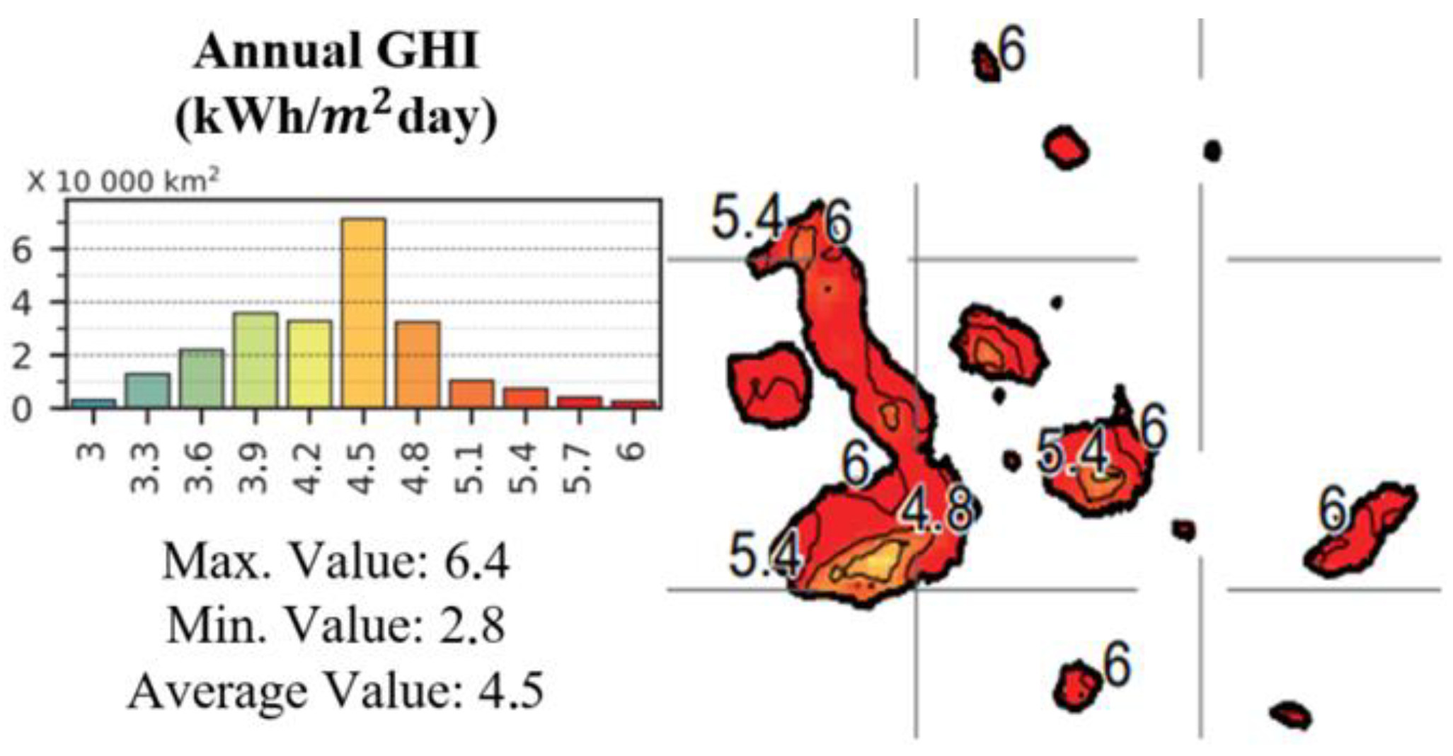
Furthermore, due to the exceptional location of the Galapagos Islands, their global horizontal irradiance (GHI) is the highest in Ecuador. As shown in Figure 2, the GHI reaches values between 4.8–6.3 kWh/m2 per day, which suggests the high feasibility of implementing solar systems in the diversification of the energy matrix of the islands [31]. Additionally, in ref. [34], it is concluded that the installation of autonomous systems in Ecuador does not represent an economic benefit for the user. However, this statement does not apply to sectors without connection with the SNI, such as the Galapagos Islands.

3. Deep Learning Techniques Applied to Forecast Photovoltaic Power

DL techniques have been widely used in the prediction of renewable energy. These have proven efficient in extracting and analyzing time series data’s nonlinear and non-stationary characteristics. Several DL variants have been developed in recent years that, unlike traditional RNN-based models, solve the vanishing gradient problem. These variants include Long Short-Term Memory Networks (LSTM), LSTM Projected (LSTMP), Bidirectional LSTM (BiLSTM), and Gated Recurrent Unit (GRU). Additionally, models based on Convolutional Neural Networks (CNN) and Hybrid models [14]. Next, DL techniques that automatically learn the characteristics necessary to forecast PV power are briefly described.

3.1. Long-Short-Term Memory Projected

In LSTM, there are a large number of computations in various gates that make up the neural network. Therefore, increasing the number of memory cells increases the memory cost. Nevertheless, you have poor neural network performance if you want to avoid this situation by preserving a low number of memory cells. From here comes the architecture called LSTMP, which improves the model’s accuracy and effectively reduces the computational load. A projected layer is a type of deep learning layer that enables compression by reducing the number of stored learning parameters. By reducing the number of parameters that can be learned by the number of hidden units of the LSTM layer, it maintains the output size of the layer and, in turn, the sizes of subsequent layers, which can result in better accuracy of the prediction layer. The LSTMP model is shown in Figure 3, where the forget gate (ft) decides if the information is retained or discarded before adding it as input to the cell; the input gate (it) controls the flow of input activations to the cell memory; the candidate memory cell ( C ˜ t ) creates a vector of new candidate values to add to the cell; the output gate (ot) controls the output flow of activations from the cell to the rest of the network; and pt is the recurrent projected activation unit [38]. In addition, the LSTMP functions are shown in ref. [39].

3.2. Bidirectional Long-Short-Term Memory

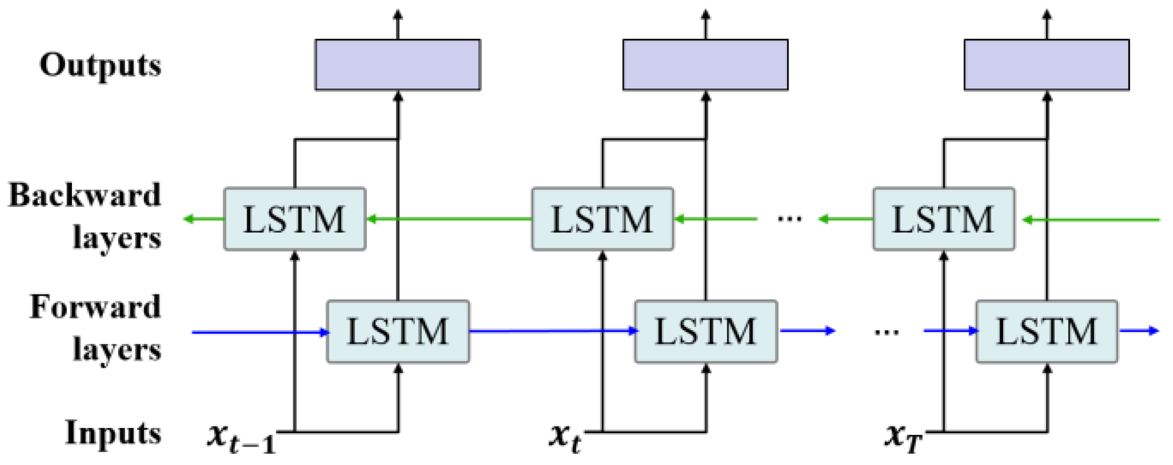
The bidirectional LSTM is an extension of the LSTM model in which two LSTM are applied to the input data. First, an LSTM is used on the input sequence (forward layer). Second, the reverse form of the input data is fed into the LSTM model (backward layer). Applying the LSTM twice improves learning long-term dependencies and consequently enhances the model’s accuracy. Likewise, a longer training time is required [40]. The Bi LSTM model is shown in Figure 4.

3.3. Convolutional Neural Network

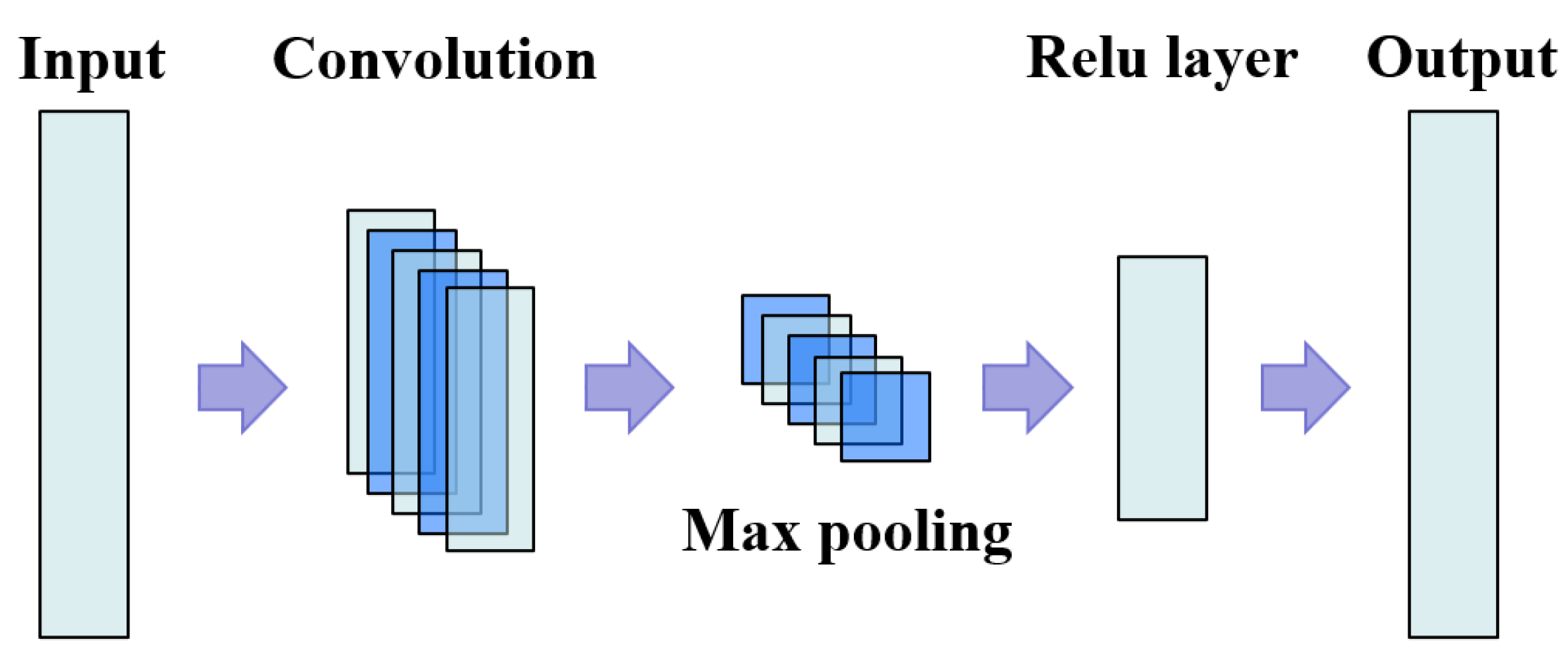
A CNN comprises two layers: convolutional and max pooling. Each layer combines the input with a weight matrix with a pre-specified size, called a filter, that defines the number of nodes that share weights to compute a feature map. These layers are achieved by sliding the weight matrix over the input and computing the dot product between the input and the weight matrix. The CNN model is shown in Figure 5. The CNN functions are presented in detail in ref. [18].
The max pooling layer computes the maximum value of the selected pool of adjacent neurons from the convolutional layer. Combining a convolutional and max pooling layer ensures that the output of the max pooling layer is invariant to shifts in the input data, which is a beneficial property for processing temporal series data. Finally, the function activation Rectified Linear Unit (ReLU) is used to compute the final prediction [41].

3.4. Hybrid

The hybrid architecture uses CNN layers described before for feature extraction on input data and combines with an RNN-based model to support sequence prediction. In this work, the RNN model corresponds to the LSTM [4]. Specifically, CNN extracts the features from inputs and uses them in the LSTM architecture to output the caption [42]. The Hybrid model is shown in Figure 6.

3.5. Hyperparameters Optimization

Before DL network training, it is necessary to initialize the model’s hyperparameters to ensure the prediction model’s performance. However, selecting hyperparameters based on experience is not a practical method since it involves attempts that require a lot of time and high computational costs and does not ensure the maximum performance of the models [24]. Optimization refers to finding the maximum or minimum of the objective function with a given set of parameter combinations. Therefore, each prediction method requires hyperparameters for its training stage. The BO is an algorithm based on a probabilistic model to find the minimum of the loss function of the DL model. The algorithm is described below:
  • A random sampling of hyperparameter values.
  • Observe the performance of the model.
  • Based on the previous observation, it fits a Gaussian process.
  • Calculate the mean of this Gaussian process as an approximation of the loss function.
  • An acquisition function (hyperparameter) obtains the following hyperparameter space exploration algorithm.
  • Fit the model, observe the output (model performance), and iterate over the same process until reaching the maximum number of iterations.
The algorithm uses the information from the previous execution to inform the following ones, which allows for reducing the search for hyperparameters throughout the process [43]. Bayesian learning offers advantages over the conventional maximum likelihood approach to training. First, a single weight vector is found, which minimizes the error function. In contrast, the Bayesian scheme considers a probability distribution over the weights, described by a prior distribution p(W) that is modified when the data D is observed, p(D). The process is expressed by the Bayes theorem (1) [21], as follows:
p ( D W ) = p ( D W ) p ( W ) p ( D )
The expressions for the prior p(W) and the likelihood p(D|W) are needed to evaluate the posterior distribution. The previous over-weights should reflect the knowledge, if any, about the mapping to be built. The model is described in ref. [21]. The procedure reasonably estimates the probability mass attached to the posterior. The development of the acquisition functions is described in ref. [44].
The data required for implementing the algorithm is divided according to the Hold-out method. This method divides the data set into training, validation, and testing. When using the Hold-out method, giving each data set a representative part of the entire data set is essential. Otherwise, the model would perform poorly on previously unseen data. Hold-out is an ML technique used to avoid overfitting or underfitting in developed models [45].

4. Methodology

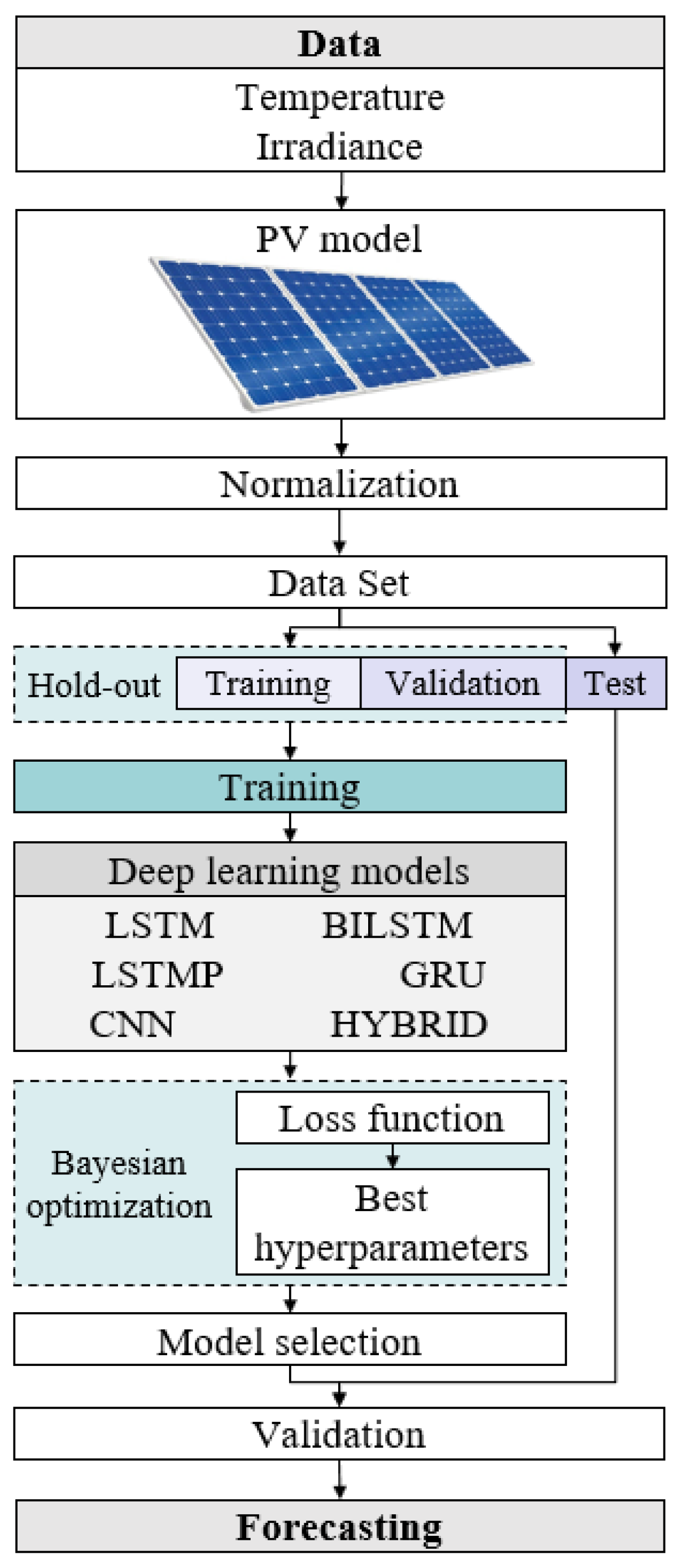
The methodology followed in this work to predict photovoltaic energy is shown in the flowchart in Figure 7.
As shown in Figure 7, the PV model obtains the generated power after collecting the weather conditions (solar irradiance and temperature) at a given location. Furthermore, data normalization is performed to get the initial data set. After that, the data set is divided into two: one for training and the other for validation. Here, the data enters different deep-learning models to perform the training, optimization, model selection, and verification processes. Next, the various stages involved in the process are developed.

4.1. Data Collection

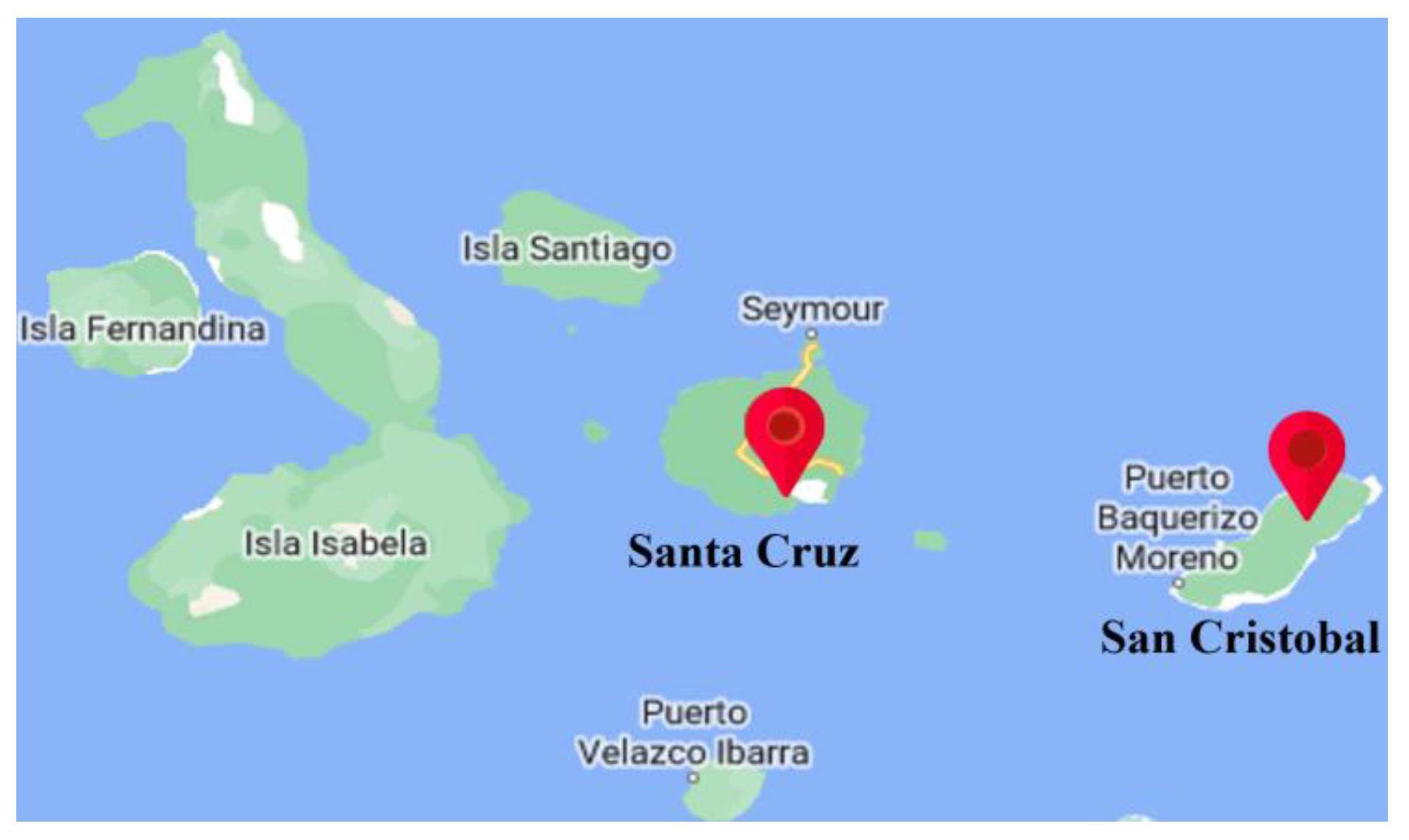
As mentioned in the section on Renewable Energies in Ecuador, the Galapagos Islands constitute a feasible location for implementing isolated systems based on NCRE. Therefore, the sites on Santa Cruz Island (0°41′42″ S 90°19′44.399″ W) correspond to Data Set 1, and San Cristobal Island (0°54′0″ S 89°30′21.6″ W) correspond to Data Set 2. Therefore, these are taken as a case study (see Figure 8). Additionally, these islands are the most populated. This study uses the data provided by the Photovoltaic Geographical Information System (PVGIS) web portal [46], which comprises hourly irradiance and temperature values from 2018 to 2020. These data serve as parameters for obtaining the PV-generated power using the model presented in (2) and(3).

4.2. Photovoltaic Model

The output power of a PV module (PPV), considering the incident irradiance, temperature, and construction material, is expressed as follows [4,47]:
P P V = P S T C G ( β , α ) G S T C 1 + γ ( T C + T S T C )
T C = ( T a 273 ) + G ( β , α ) 800 ( N O C T 20 )
where PSTC is the PV module output power under standard test conditions (STC), G(β,α) is the incident irradiance on the plane of the panels, GSTC is the incident irradiance under STC, γ is the power temperature coefficient, TSTC is the temperature under STC (°C), TC is the cell temperature (°C), Ta is the ambient temperature, and NOCT is the Nominal Operating Cell Temperature [4].
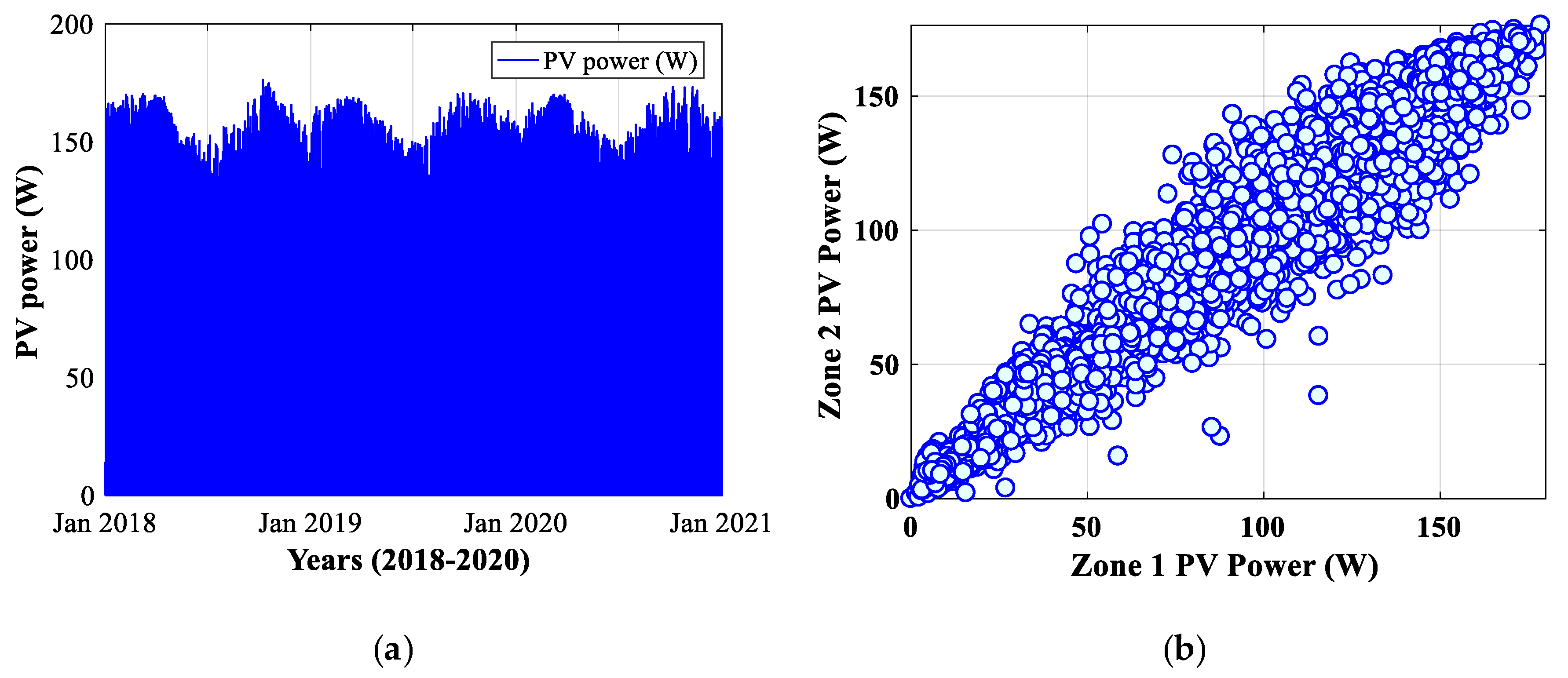
On the one hand, Figure 9a shows the PV power using Data Set 1 (location 1), where seasonal variation is observed from 2018 to 2020. On the other hand, due to the geographical proximity of both islands (Santa Cruz and San Cristobal), there are similar weather conditions. Consequently, the obtained PV power for location 2 reaches close values, which can be verified when analyzing the correlation graph, see Figure 9b, of PV power achieved in location 1 and location 2. Therefore, this study considers Data Set 1 (location 1) for getting the optimized hyperparameters.

4.3. Data Normalization

The data set is divided into 80% for training (PVTrain) and 20% for validation (PVTest). The input data consists of PV power output ranging from 0 to rated output power. Therefore, when handling some high-value data with the RNN-based model, a gradient explosion can negatively affect the model’s performance, reducing the learning efficiency. Thus, the input data is normalized through min-max normalization within the interval [0, 1] to solve this problem. Later, the data is used to build the DL models [14]. The original data normalization is defined as follows:
P V N O R M ( i ) = P V T r a i n ( i ) P V m i n P V m a x P V m i n
where PVNORM is the normalized PV power value at sample i, PVTrain is the PV power value in the data set at sample i, PVmin is the smallest PV power value in the data set, and PVmax is the most considerable PV power value in the data set.

4.4. Training

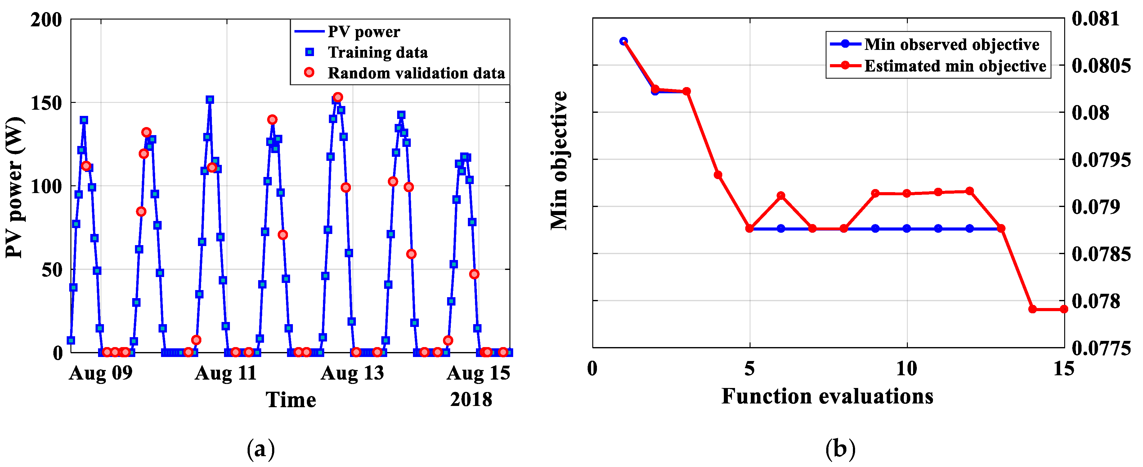
The LSTM, LSTMP, BiLSTM, GRU, CNN, and Hybrid models are trained in a supervised manner. The BO is used to obtain the training hyperparameters. Using the Hold-out method, PVTrain is divided into 80% for training, PVTrain_t, and 20% for validation, PVTrain_v. The selection of samples is carried out randomly, as shown in Figure 10a. On the other hand, Figure 10b shows the evolution of the optimal hyperparameters for the hybrid method, where the values with the lowest loss value are chosen. The Adam optimizer is used for all processes to minimize the training loss of function.
Table 1 shows the values of the optimal hyperparameters obtained for the six methods. For the LSTMP method, Var.1 and Var.2 correspond to the output and input projector sizes, respectively. The CNN and hybrid Var.1 and Var.2 correspond to the size of the filter and the number of filters, respectively. It is worth noting that for the hybrid method, fewer values are required for feature extraction than the CNN method, which does not include the RNN layer.

4.5. Performance Indicators

Performance indicators are used to quantify the results of the different methods. As in many works, the Root Mean Square Error (RMSE) (5), Mean Absolute Error (MAE) (6), Mean Absolute Percentage Error (MAPE) (7), and correlation coefficient (Cor. Coef.) (8) are used. These indicators have been defined in ref. [4]. However, here they are recalled for the sake of paper completeness.
R M S E = 1 n i = 1 n ( y i y ^ l ) 2
M A E = 1 n i = 1 n y i y ^ l
M A P E = 100 n i = 1 n y i y ^ l y i
C o r . c o e f . = 1 n 1 i = 1 n y i μ y i σ y i y ^ l μ y ^ l σ y ^ l
where n is the sample number, yi is the real power value at sample i, y ^ l is the predicted power value at sample i, μyi and σyi are the real power’s mean and standard deviation, respectively, and μ y ^ l and σ y ^ l are the expected power’s mean and standard deviation, respectively [4].

5. Simulation Results

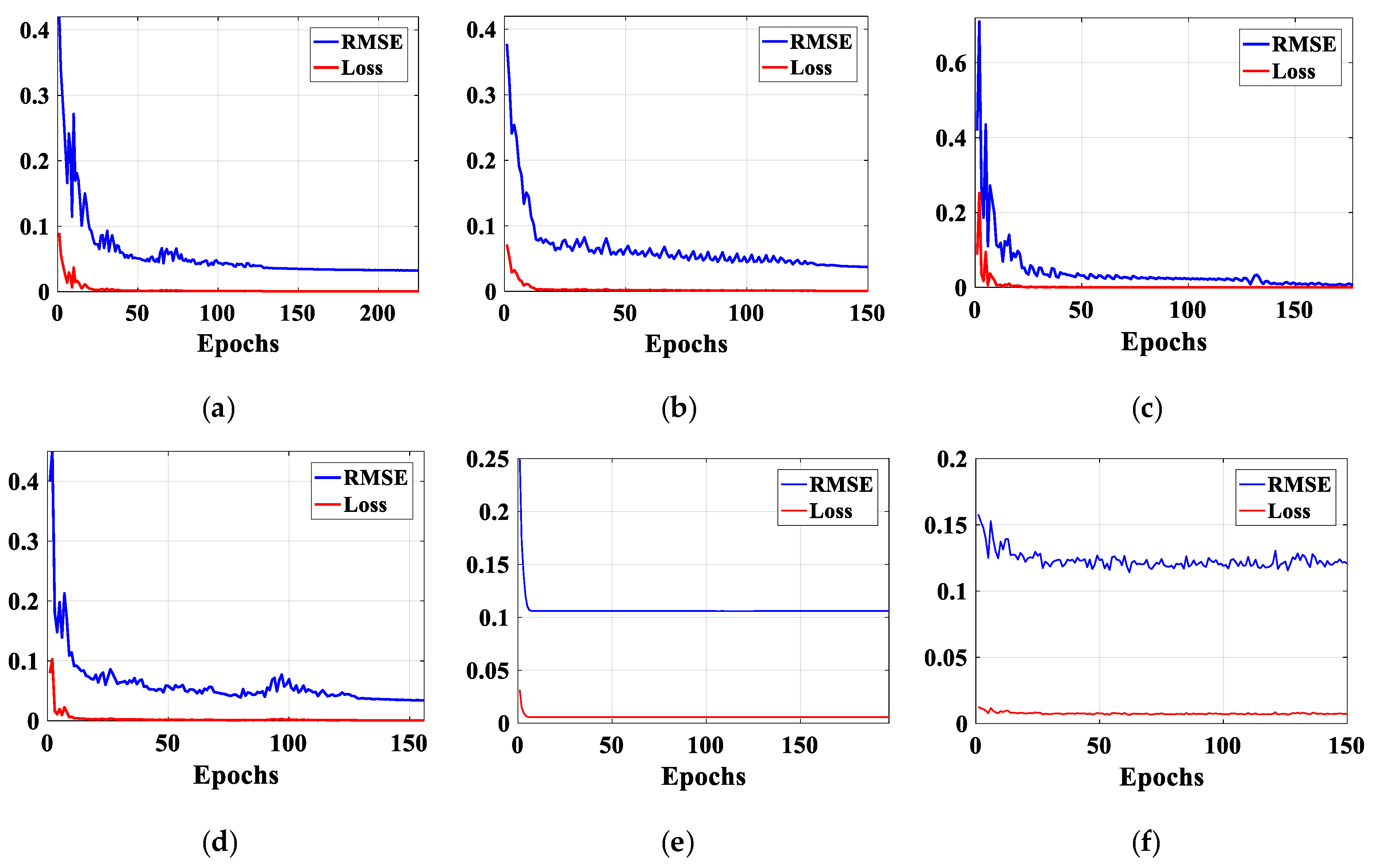
The presented DL techniques applied to forecast PV power are simulated in Matlab®® using a computer with an Intel®® Core™ i7-3770 processor and 8GB of RAM. Figure 11 shows the models’ training metrics for Data Set 1.
As seen in Figure 11, the error value decreases according to the optimized number of iterations. Additionally, the loss function value does not show fluctuations after the optimized number of epochs, which implies that the parameters are already well-learned for prediction. Moreover, the CNN model, shown in Figure 11e, presents a smoother training curve than the other models since the filter size is applied to the input data, in contrast to the RRN-based models that deal with the temporal changes of the PV power. The methods reached a Loss value close to 0, implying a precise model and minimizing the forecast error.
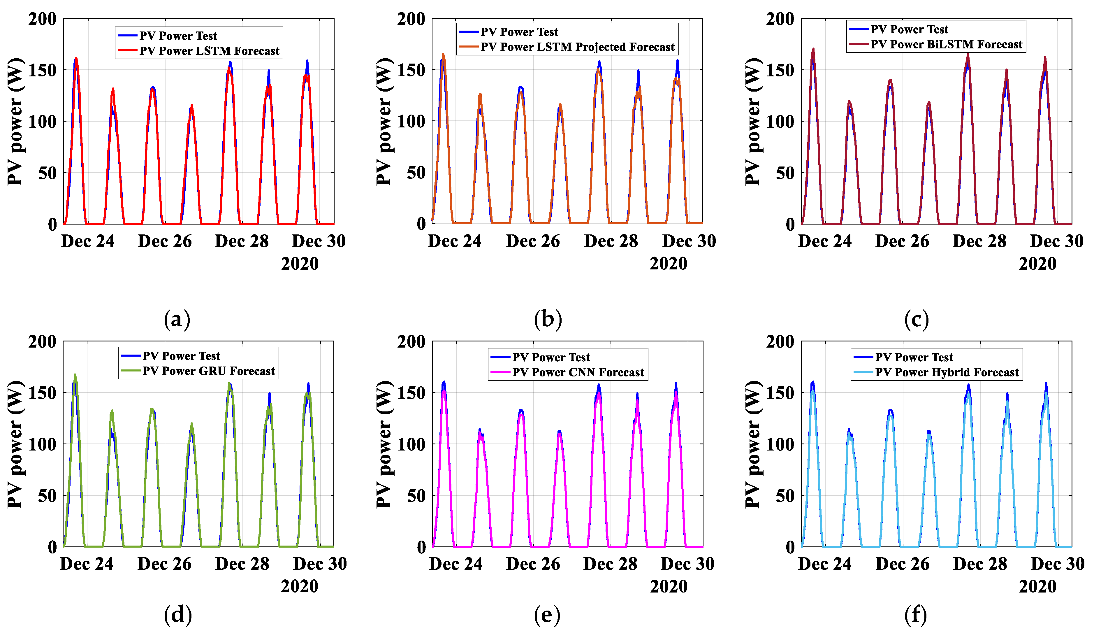
In addition, Figure 12 shows the actual and predicted PV power achieved in one week using Data Set 1 through the LSTM, LSTM Projected, BiLSTM, GRU, CNN, and Hybrid methods.
It is worth noting that all methods present an excellent approximation between the actual and forecasted PV power.
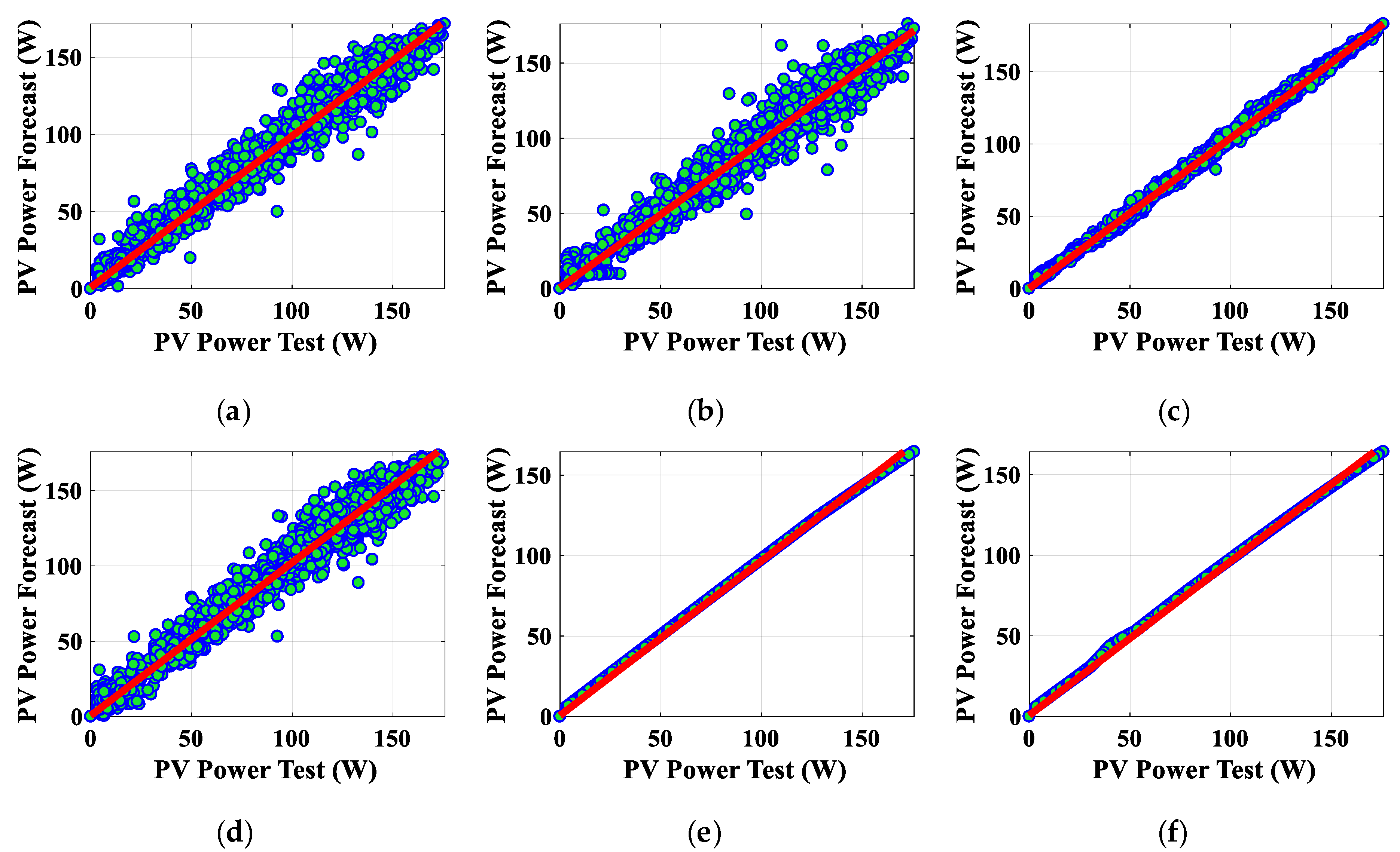
Furthermore, Figure 13 shows the correlation graph between the real and predicted PV power for all methods for the entire validation period using Data Set 1.
As shown in Figure 13, the results imply a significant linear dependence between the variables. Similar results are obtained with the LSTM, LSTMP, and GRU methods. However, the results achieved by BiLSTM, CNN, and Hybrid methods show improved performance since the predicted values are closer to the actual ones. These results demonstrate that all methods with optimized hyperparameters are efficient for the forecast task.
Performance indicators are used further to assess one method’s quantitative advantages. As evidenced in Table 2, all the methods analyzed manage to make an efficient short-term prediction of PV power.
The results presented in Table 2 show that the RMSE value is small, indicating a high prediction precision. Furthermore, the MAE and MAPE metrics indicate a low difference between the predicted and actual values. On the other hand, the Cor. Coef. obtained value is close to 1, which means a significant linear dependence between the real and predicted values.
Conversely, Figure 14 shows the correlation graph considering Data Set 2.
In the same way, as with the results obtained with Data Set 1, the models present the same accuracy on the forecast. Again, BiLSTM, CNN, and Hybrid show improved performance.
Moreover, the performance indicators for Data Set 2 are presented in Table 3.
It can be noticed from Table 3 that the obtained error values are low and similar to those obtained with Data Set 1. Furthermore, Bayesian optimization demonstrated that it was capable of getting optimized hyperparameters for the eight DL models, which can be used in the forecasting task in the isolated areas used as case studies. Due to the low error obtained in the forecast for both Data sets, the methodology applied in this work demonstrated that it was capable of bringing precise DL models.
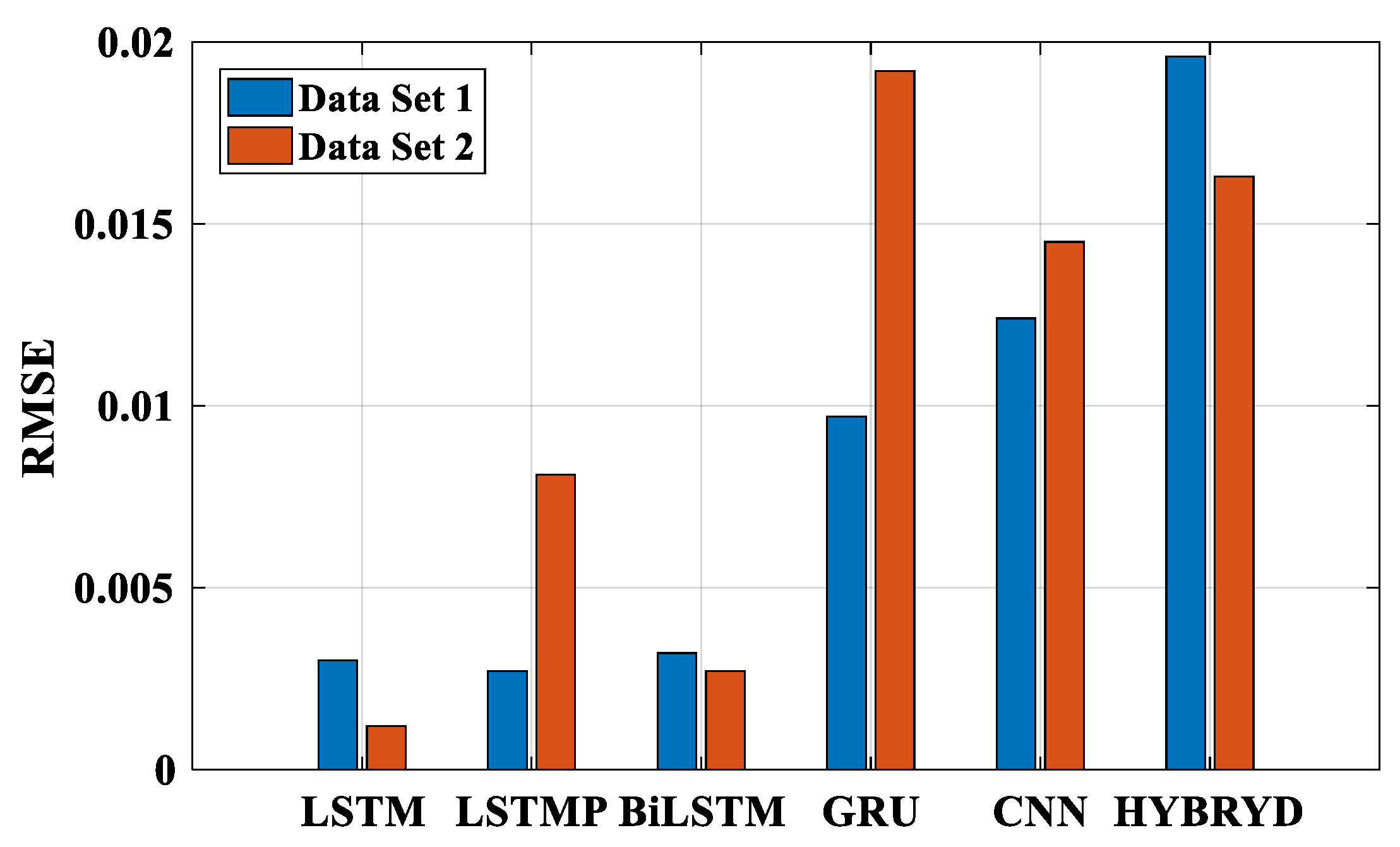
Additionally, Figure 15 compares the obtained RMSE values for all models for both data sets.
It can be seen in Figure 15 that the LSTM model gets a lower value than BiLSTM, indicating that the characteristics of the temporal series do not need to go backward. Feedforward layers are to be learned, but the models above better captured the temporary changes’ features in contrast with GRU, CNN, and Hybrid, which get higher RMSE values in the forecast.
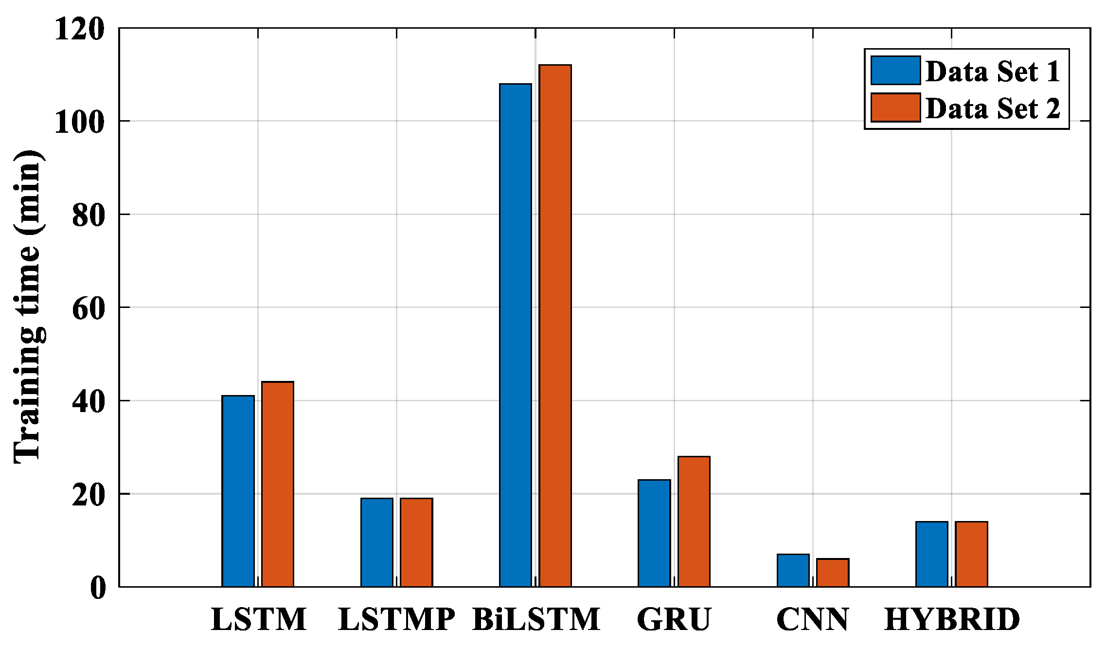
Moreover, Table 4 compares the training time for all models to evaluate the computational performance, whereas Figure 16 shows a visual representation of these values.
As can be seen in Table 4 and Figure 16, the LSTMP, GRU, CNN, and Hybrid models obtain the lowest training times. In contrast, the LSTM and BiLSTM models present higher training times. Specifically, the BiLSTM model got the highest training time since this method uses backward and feedforward layers (two LSTM cells) to learn. However, since it obtains higher RMSE values, the double-layer feature is unnecessary for the data type used in this work.
It is worth noting that due to the LSTM model achieving the lowest RMSE value in the forecast and training time, the model developed with the optimized hyperparameters can adequately learn the temporal changes of the photovoltaic power in both locations under study in contrast with the other models.
Furthermore, Table 5 compares the LSTM and GRU methods’ results and their hyperparameters.
As seen in Table 5, the BO reduced the number of epochs for both methods, which implies a reduction in computational cost. Furthermore, for the LSTM method, the number of hidden units (NHU) is decreased, resulting in reduced network complexity. However, the NHU is increased for the GRU method, which implies that the model requires more hidden layers to learn the PV power’s temporal changes. Finally, it is worth noting that the performance of the methods with optimized hyperparameters has lower error values and higher correlation coefficients. Therefore, the BO allows improved DL methods and more accurate models with reduced hyperparameter values and computational costs.

6. Conclusions

This work presents six short-term PV power forecasting models based on deep learning techniques. The study has been developed for two geographically close and remote areas (Santa Cruz and San Cristobal Islands) in the Galapagos Islands of Ecuador. The proposed methodology has proven efficient for LSTM, LSTMP, BiLSTM, CNN, and Hybrid training tasks based on the prediction accuracy obtained and the decreased computational cost. Nevertheless, the procedure could be used to get a forecast of PV power in many areas with this prerequisite. Furthermore, performance indicators for all techniques have shown very low RMSE and excellent 99% correlations between actual PV and resulting forecast values in both data sets.
In addition, Bayesian optimization has helped to obtain the necessary hyperparameters for model training, reducing the error in the forecast task and the training time. Finally, simulation results have demonstrated that LSTM, LSTMP, BiLSTM, GRU, CNN, and Hybrid methods are efficient in the short-term forecasting of PV power. Nevertheless, LSTM has improved performance in learning temporal changes. Therefore, the results can be used as a reference for implementing remote solar PV systems in the Galapagos Islands.

Author Contributions

Conceptualization, R.G., D.A.-A. and M.F.-C.; data curation R.G.; formal analysis D.A.-A., M.F., W.M. and F.G.; investigation R.G. and D.A.A.; methodology R.G., D.A.-A. and M.F.-C.; project administration D.A.-A. and W.M.; software R.G.; supervision D.A.-A. and M.F.-C.; validation D.A.-A., M.F.-C., W.M. and F.G.; visualization R.G.; writing—original draft preparation R.G., D.A.-A., M.F.-C., W.M. and F.G; writing—review and editing D.A.-A. and M.F.-C. All authors have read and agreed to the published version of the manuscript.

Funding

This work is part of the projects 2023-PIS-004, 2022-PIJ-10, and 2020-EXT-007 “MIRA-ESTE: Specific, innovative microgrids solutions (accounting for environmental, social, technological and economic aspects) for isolated rural areas of Ecuador” from the Research Group of Propagation, Electronic Control, and Networking (PROCONET) of Universidad de las Fuerzas Armadas ESPE and KU Leuven. This work has been developed with the support of VLIR-UOS and the Belgian Development Cooperation (DGD) under the project EC2020SIN322A101.

Institutional Review Board Statement

Not applicable.

Informed Consent Statement

Not applicable.

Data Availability Statement

The data presented in this study are available on request from the corresponding author.

Conflicts of Interest

The authors declare no conflict of interest.

References

  1. Luo, X.; Zhang, D. An adaptive deep learning framework for day-ahead forecasting of photovoltaic power generation. Sustain. Energy Technol. Assess. 2022, 52, 102326. [Google Scholar] [CrossRef]
  2. Etxegarai, G.; López, A.; Aginako, N.; Rodríguez, F. An analysis of different deep learning neural networks for intra-hour solar irradiation forecasting to compute solar photovoltaic generators’ energy production. Energy Sustain. Dev. 2022, 68, 1–17. [Google Scholar] [CrossRef]
  3. Rodríguez, F.; Azcárate, I.; Vadillo, J.; Galarza, A. Forecasting intra-hour solar photovoltaic energy by assembling wavelet based time-frequency analysis with deep learning neural networks. Int. J. Electr. Power Energy Syst. 2022, 137, 107777. [Google Scholar] [CrossRef]
  4. Guanoluisa-Pineda, R.; Ibarra, A.; Arcos-Aviles, D.; Martinez, W.; Motoasca, E.; Guinjoan, F. Short-Term forecasting of photovoltaic power in an isolated area of Ecuador using deep learning techniques. In Proceedings of the 11th International Conference on Renewable Energy Research and Application, Istanbul, Turkey, 18–21 September 2022; pp. 408–413. [Google Scholar] [CrossRef]
  5. Aribia, H.B.; El-Rifaie, A.M.; Tolba, M.A.; Shaheen, A.; Moustafa, G.; Elsayed, F.; Elshahed, M. Growth Optimizer for Parameter Identification of Solar Photovoltaic Cells and Modules. Sustainability 2023, 15, 7896. [Google Scholar] [CrossRef]
  6. Elshahed, M.; El-Rifaie, A.M.; Tolba, M.A.; Ginidi, A.; Shaheen, A.; Mohamed, S.A. An Innovative Hunter-Prey-Based Optimization for Electrically Based Single-, Double-, and Triple-Diode Models of Solar Photovoltaic Systems. Mathematics 2022, 10, 4625. [Google Scholar] [CrossRef]
  7. Shaheen, A.; El-Sehiemy, R.; El-Fergany, A.; Ginidi, A. Representations of solar photovoltaic triple-diode models using artificial hummingbird optimizer. Energy Sources Part A Recover Util. Environ. Eff. 2022, 44, 8787–8810. [Google Scholar] [CrossRef]
  8. El-Sehiemy, R.; Shaheen, A.; El-Fergany, A.; Ginidi, A. Electrical parameters extraction of PV modules using artificial hummingbird optimizer. Sci. Rep. 2023, 13, 9240. [Google Scholar] [CrossRef]
  9. Ginidi, A.R.; Shaheen, A.M.; El-Sehiemy, R.A.; Hasanien, H.M.; Al-Durra, A. Estimation of electrical parameters of photovoltaic panels using heap-based algorithm. IET Renew. Power Gener. 2022, 16, 2292–2312. [Google Scholar] [CrossRef]
  10. Eidiani, M.; Zeynal, H.; Ghavami, A.; Zakaria, Z. Comparative Analysis of Mono-Facial and Bifacial Photovoltaic Modules for Practical Grid-Connected Solar Power Plant Using PVsyst. In Proceedings of the IEEE International Conference on Power Energy, Langkawi, Kedah, Malaysia, 5–6 December 2022; pp. 499–504. [Google Scholar] [CrossRef]
  11. Pascual, J.; Barricarte, J.; Sanchis, P.; Marroyo, L. Energy management strategy for a renewable-based residential microgrid with generation and demand forecasting. Appl. Energy 2015, 158, 12–25. [Google Scholar] [CrossRef]
  12. Kanchana, W.; Sirisukprasert, S. PV Power Forecasting with Holt-Winters Method. In Proceedings of the 8th International Electrical Engineering Congress (iEECON) 2020, Chiang Mai, Thailand, 4–6 March 2020; pp. 1–4. [Google Scholar] [CrossRef]
  13. Hossain, M.S.; Mahmood, H. Short-Term Photovoltaic Power Forecasting Using an LSTM Neural Network and Synthetic Weather Forecast. IEEE Access 2020, 8, 172524–172533. [Google Scholar] [CrossRef]
  14. Dairi, A.; Harrou, F.; Sun, Y.; Khadraoui, S. Short-Term Forecasting of Photovoltaic Solar Power Production Using Variational Auto-Encoder Driven Deep Learning Approach. Appl. Sci. 2020, 10, 8400. [Google Scholar] [CrossRef]
  15. Cheng, L.; Zang, H.; Wei, Z.; Ding, T.; Sun, G. Solar Power Prediction Based on Satellite Measurements—A Graphical Learning Method for Tracking Cloud Motion. IEEE Trans. Power Syst. 2022, 37, 2335–2345. [Google Scholar] [CrossRef]
  16. Rodríguez, F.; Galarza, A.; Vasquez, J.C.; Guerrero, J.M. Using deep learning and meteorological parameters to forecast the photovoltaic generators intra-hour output power interval for smart grid control. Energy 2022, 239, 122116. [Google Scholar] [CrossRef]
  17. Suresh, V.; Janik, P.; Rezmer, J.; Leonowicz, Z. Forecasting Solar PV Output Using Convolutional Neural Networks with a Sliding Window Algorithm. Energies 2020, 13, 723. [Google Scholar] [CrossRef] [Green Version]
  18. Agga, A.; Abbou, A.; Labbadi, M.; El Houm, Y. Short-term self consumption PV plant power production forecasts based on hybrid CNN-LSTM, ConvLSTM models. Renew. Energy 2021, 177, 101–112. [Google Scholar] [CrossRef]
  19. Zhou, S.; Zhou, L.; Mao, M.; Xi, X. Transfer Learning for Photovoltaic Power Forecasting with Long Short-Term Memory Neural Network. In Proceedings of the International Conference on Big Data and Smart Computing, Busan, Republic of Korea, 12–22 February 2020; pp. 125–132. [Google Scholar] [CrossRef]
  20. Klein, A.; Falkner, S.; Bartels, S.; Hennig, P.; Hutter, F. Fast Bayesian hyperparameter optimization on large datasets. Electron. J. Stat. 2017, 11, 4945–4968. [Google Scholar] [CrossRef]
  21. Ciaramella, A.; Staiano, A.; Cervone, G.; Alessandrini, S. A Bayesian-Based Neural Network Model for Solar Photovoltaic Power Forecasting. In Advances in Neural Networks: Computational Intelligence for ICT; Bassis, S., Esposito, A., Morabito, F., Pasero, E., Eds.; Springer: Cham, Switzerland, 2016; pp. 169–177. [Google Scholar] [CrossRef]
  22. Guo, X.; Mo, Y.; Yan, K. Short-Term Photovoltaic Power Forecasting Based on Historical Information and Deep Learning Methods. Sensors 2022, 22, 9630. [Google Scholar] [CrossRef]
  23. Li, Y.; Li, Z.; Yang, L.; Wang, B. Photovoltaic Power Prediction Based on Improved Sparse Bayesian Regression. Electr. Power Compon. Syst. 2016, 44, 1958–1968. [Google Scholar] [CrossRef]
  24. Jin, X.-B.; Zheng, W.-Z.; Kong, J.-L.; Wang, X.-Y.; Bai, Y.-T.; Su, T.-L.; Lin, S. Deep-Learning Forecasting Method for Electric Power Load via Attention-Based Encoder-Decoder with Bayesian Optimization. Energies 2021, 14, 1596. [Google Scholar] [CrossRef]
  25. Zhang, R.; Ma, H.; Hua, W.; Saha, T.K.; Zhou, X. Data-Driven Photovoltaic Generation Forecasting Based on a Bayesian Network With Spatial–Temporal Correlation Analysis. IEEE Trans. Ind. Inform. 2020, 16, 1635–1644. [Google Scholar] [CrossRef]
  26. Afshin, M.; Sadeghian, A.; Raahemifar, K. On Efficient Tuning of LS-SVM Hyper-Parameters in Short-Term Load Forecasting: A Comparative Study. In Proceedings of the IEEE Power Engineering Society General Meeting, Tampa, FL, USA, 24–28 June 2007; pp. 1–6. [Google Scholar] [CrossRef]
  27. Levman, J.; Jennings, M.; Kabaria, P.; Rouse, E.; Nangaku, M.; Berger, D.; Gondra, I.; Takahashi, E.; Tyrrell, P. Hold-out validation for the assessment of stability and reliability of multivariable regression demonstrated with magnetic resonance imaging of patients with schizophrenia. Int. J. Dev. Neurosci. 2021, 81, 655–662. [Google Scholar] [CrossRef] [PubMed]
  28. Enriquez, E. Diseño y Simulación de un Sistema de Previsión de Generación Fotovoltaica Basado en la Predicción Numérica del Clima. Bachelor’s Thesis, Universidad de las Fuerzas Armadas ESPE, Sangolquí, Ecuador, 2019. [Google Scholar]
  29. Fabara, C.; Maldonado, D.; Soria, M.; Tovar, A. Predicción de la Generación para un Sistema Fotovoltaico mediante la aplicación de técnicas de Minería de Datos. Rev. Técnica Energía 2019, 16, 64–72. [Google Scholar] [CrossRef]
  30. Romero, A.F.; Quilumba, F.L.; Arcos, H.N. Short-term active power forecasting of a photovoltaic power plant using an artificial neural network. In Proceedings of the Second Ecuador Technical Chapters Meeting, Salinas, Ecuador, 16–20 October 2017; pp. 1–5. [Google Scholar] [CrossRef]
  31. Vaca, D.; Ordoñez, F. Mapa Solar del Ecuador 2019. Quito. 2019. Available online: https://www.ingenieriaverde.org/wp-content/uploads/2020/01/Mapa_Solar_del_Ecuador_2019.pdf (accessed on 20 November 2022).
  32. Rodriguez, M.; Arcos–Aviles, D.; Martinez, W. Fuzzy logic-based energy management for isolated microgrid using meta-heuristic optimization algorithms. Appl. Energy 2023, 335, 120771. [Google Scholar] [CrossRef]
  33. ARCERNNR. ATLAS del Sector Eléctrico Ecuatoriano. Quito. 2021. Available online: Chrome-extension://efaidnbmnnnibpcajpcglclefindmkaj/https://www.controlrecursosyenergia.gob.ec/wp-content/uploads/downloads/2022/04/Atlas2021.pdf (accessed on 15 December 2022).
  34. Rodríguez, M.; Salazar, A.; Arcos-Aviles, D.; Llanos, J.; Martínez, W.; Motoasca, E. A Brief Approach of Microgrids Implementation in Ecuador: A Review. In XV Multidisciplinary International Conference on Intelligent Information Technology; Botto Tobar, M., Cruz, H., Díaz Cadena, A., Eds.; CIT 2020 Press: Quito, Ecuador; Springer: Cham, Switzerland, 2021; pp. 149–163. [Google Scholar] [CrossRef]
  35. Ayala-Pico, J.; Arcos–Aviles, D.; Ibarra, A.; Fernandez, C.; Guinjoan, F.; Martinez, W. Current development of electricity generation systems in the Galapagos Islands—Ecuador. Renew. Energy Focus 2023, 46, 88–102. [Google Scholar] [CrossRef]
  36. MEER. Plan Nacional de Eficiencia Energética 2016–2035; MEER: Quito, Ecuador, 2017. [Google Scholar]
  37. ElecGalapagos. Rendición de Cuentas; ElecGalapagos: San Cristobal, Galápagos, Ecuador, 2021. [Google Scholar]
  38. Jia, Y.; Wu, Z.; Xu, Y.; Ke, D.; Su, K. Long Short-Term Memory Projection Recurrent Neural Network Architectures for Piano’s Continuous Note Recognition. J. Robot. 2017, 2017, 1–7. [Google Scholar] [CrossRef] [Green Version]
  39. Sak, H.; Senior, A.; Beaufays, F. Long Short-Term Memory Based Recurrent Neural Network Architectures for Large Vocabulary Speech Recognition. arXiv 2014, arXiv:1402.1128v1. [Google Scholar] [CrossRef]
  40. Siami-Namini, S.; Tavakoli, N.; Namin, A.S. The Performance of LSTM and BiLSTM in Forecasting Time Series. In Proceedings of the International Conference on Big Data (Big Data), Los Angeles, CA, USA, 9–12 December 2019; pp. 3285–3292. [Google Scholar] [CrossRef]
  41. Koprinska, I.; Wu, D.; Wang, Z. Convolutional Neural Networks for Energy Time Series Forecasting. In Proceedings of the International Joint Conference on Neural Networks, Rio de Janeiro, Brazil, 8–13 July 2018; pp. 1–8. [Google Scholar] [CrossRef]
  42. Rajagukguk, R.A.; Ramadhan, R.A.A.; Lee, H.-J. A Review on Deep Learning Models for Forecasting Time Series Data of Solar Irradiance and Photovoltaic Power. Energies 2020, 13, 6623. [Google Scholar] [CrossRef]
  43. Cavazza, M. Towards Data Science. 2021. Available online: https://medium.com/towards-data-science/improve-your-model-performance-with-bayesian-optimization-hyperparameter-tuning-4dbd7fe25b62 (accessed on 20 November 2022).
  44. Kelin, A.; Falkner, S.; Bartels, S.; Henning, P.; Hutter, F. Fast Bayesian Optimization of Machine Learning Hyperparameters on Large Datasets. In Proceedings of the International Conference on Artificial Intelligence and Statistics, Fort Lauderdale, FL, USA, 20–22 April 2017; pp. 1–9. [Google Scholar]
  45. Kumar, A. Data Analytics 2022. Available online: https://vitalflux.com/hold-out-method-for-training-machine-learning-model/ (accessed on 15 November 2022).
  46. Commission, E. Photovoltaic Geographical Information System. 2019. Available online: https://re.jrc.ec.europa.eu/pvg_tools/en/#MR (accessed on 7 December 2022).
  47. Arcos-Aviles, D.; Pascual, J.; Guinjoan, F.; Marroyo, L.; Sanchis, P.; Marietta, M.P. Low complexity energy management strategy for grid profile smoothing of a residential grid-connected microgrid using generation and demand forecasting. Appl. Energy 2017, 205, 69–84. [Google Scholar] [CrossRef]
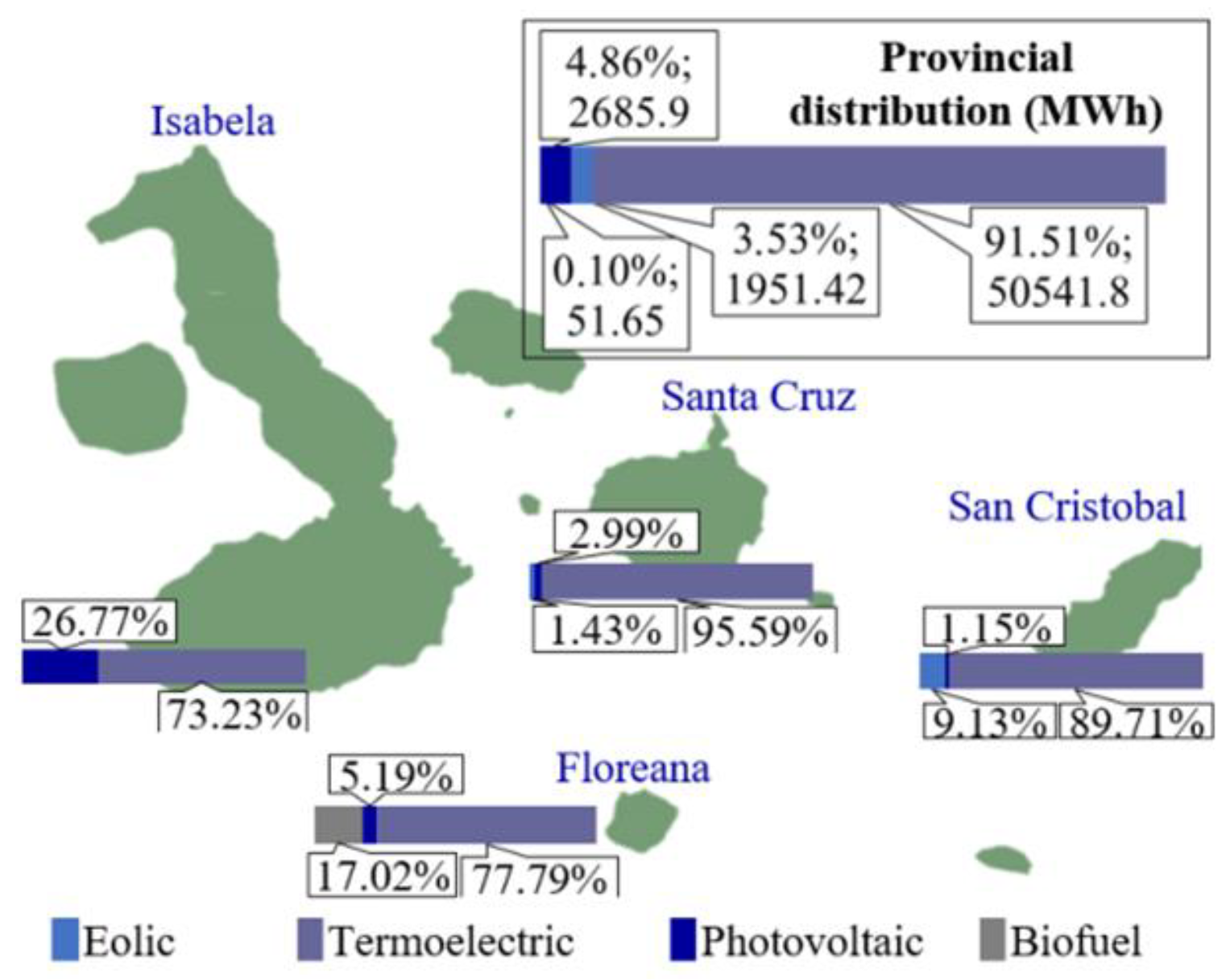
Figure 1. Electric energy generation distribution in the Galapagos Islands.
Sustainability 15 12151 g001
Figure 2. Annual global horizontal irradiance by 2021 in Galapagos Islands [31].
Sustainability 15 12151 g002
Figure 3. Long-short-term memory projected network model.
Sustainability 15 12151 g003
Figure 4. Bidirectional Long-short-term memory network model.
Sustainability 15 12151 g004
Figure 5. Convolutional neural network model.
Sustainability 15 12151 g005
Figure 6. Hybrid deep learning network model.
Sustainability 15 12151 g006
Figure 7. Forecasting flowchart.
Sustainability 15 12151 g007
Figure 8. Case study locations.
Sustainability 15 12151 g008
Figure 9. (a) Photovoltaic power of Santa Cruz Island from 2018 to 2020. (b) Correlation of the photovoltaic power between Santa Cruz and San Cristobal islands.
Sustainability 15 12151 g009
Figure 10. (a) Hold-out of the data set. (b) Bayesian optimization of Hybrid hyperparameters.
Sustainability 15 12151 g010
Figure 11. RMSE of training of DL models (a) LSTM, (b) LSTM Projected, (c) BiLSTM, (d) GRU, (e) CNN, and (f) Hybrid.
Sustainability 15 12151 g011
Figure 12. PV Real Power and Forecast Power on Data Set 1 (a) LSTM, (b) LSTM Projected, (c) BiLSTM, (d) GRU, (e) CNN, and (f) Hybrid.
Sustainability 15 12151 g012
Figure 13. Scatter graph of actual and forecasted PV power for Data Set 1 (a) LSTM, (b) LSTM Projected, (c) BiLSTM, (d) GRU, (e) CNN, and (f) Hybrid.
Sustainability 15 12151 g013
Figure 14. Scatter graph of actual and forecasted PV power for Data Set 2 (a) LSTM, (b) LSTM Projected, (c) BiLSTM, (d) GRU, (e) CNN, and (f) Hybrid.
Sustainability 15 12151 g014
Figure 15. RMSE comparison for the studied models.
Sustainability 15 12151 g015
Figure 16. Training time for DL models.
Sustainability 15 12151 g016
Table 1. Optimized hyperparameters for forecasting.
MethodEpochHidden UnitsLearning RateVar. 1Var. 2
LSTM2251590.0084568
LSTMP1592650.0099320925
BiLSTM1772540.0099758
GRU1562470.0099982
CNN197 0.00011343127
Hybrid150960.0012401917
Table 2. Performance metrics results from Data Set 1.
MethodRMSEMAEMAPECor. Coef.
LSTM0.00302.55770.55510.9962
LSTMP0.00272.56820.55420.9960
BiLSTM0.00322.62160.52060.9998
GRU0.00972.64050.56010.9961
CNN0.01242.09140.54560.9994
Hybrid0.01962.13540.52690.9994
Table 3. Performance metrics results from Data Set 2.
MethodRMSEMAEMAPECor. Coef.
LSTM0.00122.93390.58410.9951
LSTMP0.00813.16430.58470.9943
BiLSTM0.00272.05420.54700.9996
GRU0.01923.19920.58520.9948
CNN0.01451.50660.53410.9998
Hybrid0.01631.71440.53360.9997
Table 4. Computational performance.
MethodTraining Time (Min) Data Set 1 Training Time (Min) Data Set 2
LSTM4144
LSTMP1919
BiLSTM108112
GRU2328
CNN76
Hybrid1414
Table 5. Performance comparison.
MethodHyperparametersPerformance Evaluation
EpochsNHURMSECorr. Coef.
LSTM2502000.05170.9514
GRU2502000.00230.9528
LSTM optimized2251590.00300.9962
GRU optimized1562370.00970.9961
Disclaimer/Publisher’s Note: The statements, opinions and data contained in all publications are solely those of the individual author(s) and contributor(s) and not of MDPI and/or the editor(s). MDPI and/or the editor(s) disclaim responsibility for any injury to people or property resulting from any ideas, methods, instructions or products referred to in the content.