More Accurate Climate Trend Attribution by Using Cointegrating Vector Time Series Models

Abstract

Adapting to human-induced climate change is becoming an increasingly important aspect of sustainable development. To be able to do this effectively, it is important to know how much human influence has contributed to observed climate trends. Climate detection and attribution (D&A) studies achieve this by estimating scaling factors usually obtained by performing a least squares regression of the observed trending climate variable on the equivalent variable simulated by a climate model. This study proposed instead to estimate scaling factors by using the econometric approach of dynamically modelling the time series as a cointegrating Vector Auto-Regressive (VAR) time series process. It is shown that a 2nd-order cointegrating VAR(2) model is theoretically justified if the observed and simulated variables can be represented as a one-box AR(1) response to a common integrated forcing. The VAR(2) model can be expressed as a Vector Error-Correction Model (VECM) and then fitted to the data to obtain the cointegration relationship, the stationary linear combination of the two variables, from which the scaling factor is then easily obtained. Estimates of the scaling factor from the VAR(2) model are critically compared to those from Ordinary Least Squares (OLS) and Total Least Squares (TLS) for annual Global Mean Surface Temperature (GMST) data simulated by a simple stochastic model of the carbon–climate system and for historical simulations from 16 climate models in the Coupled Model Intercomparison Project 5 (CMIP5) experiment. Results from the toy model simulations show that the slope estimates from OLS are negatively biased, TLS estimates are less biased but have high variance, and the VAR(2) estimates are unbiased and have lower variance and provide the most accurate estimates with smallest mean squared error. Similar behaviour is noted in the CMIP5 data. Hypothesis tests on the VAR(2) fits found strong evidence of a cointegrating relationship with the observations for all the CMIP5 simulations.

1. Introduction

Taking urgent action to combat climate change and its impacts is a major goal of sustainable development. To be able to address this, it is important to be able to accurately quantify what fraction of a climate trend can be attributed to human influence. This study explored the accuracy of various approaches to the attribution of trends in Global Mean Surface Temperature (GMST). GMST is an important variable in attribution because: (a) changes in GMST can be directly attributed to changes in the Earth’s energy budget; (b) other climate variables and the risk of weather extremes on global and regional scales can be predicted using GMST as a climate change index [1,2]; (c) GMST is the metric of climate change used by policymakers (e.g., the global warming limits of the 2015 Paris Agreement). Quantifying the effect of different forcing agents on GMST is therefore critical for informing climate change mitigation and adaptation measures. Furthermore, this study is relevant to recent studies that are starting to use attribution for impacts of climate, e.g., heat-related trends in human health [3].

Detection and attribution studies assess whether climate change can be detected as being significantly outside the range expected from natural internal variability and assess to what extent observed changes can be attributed to external forcings of climate change, both human-induced and naturally occurring. Hegerl et al. [4] defined the detection of climate change as a process of demonstrating that the climate or a system affected by the climate has changed in some defined statistical sense without providing a reason for that change. Attribution was defined as the process of evaluating the relative contributions of multiple causal factors to a change or event with an assignment of statistical confidence. The reliable detection and attribution of changes in the climate is fundamental to our understanding of climate change and to enabling decision-makers to manage climate-related risk. Moreover, confidence in the assessment of climate change will be increased when attribution of the change to a causal factor is robustly quantified and when there is a firm understanding of the processes that are involved in the proposed causal link [4].

Current approaches to the detection and attribution of an anthropogenic influence on climate involve quantifying the level of agreement between model-predicted patterns of externally forced change and observed changes in the recent climate record [5]. Most previous studies have used a regression approach in which it is assumed that observations can be represented as a linear combination of candidate signals (the climate model simulated responses to external forcing) plus noise ([6] p. 712). The regression model has the form $\mathbf{y}=\mathbf{X}\mathit{\beta }+\mathit{ϵ}$, where $\mathbf{y}={(y_1,y_2,\dots ,y_n)}^T$ is a vector of observations, matrix $\mathbf{X}$ contains the simulated responses to the external forcings that are under investigation (with one column for each signal considered), $\mathit{\beta }$ is a vector of slope parameters (scaling factors) that adjusts the amplitudes of those patterns and $\mathit{ϵ}$ represents internal climate variability [5,7,8,9]. The unknown scaling factors, $\mathit{\beta }$, are generally estimated using either Generalized Least Squares (GLS) or Total Least Squares (TLS) estimation [8,10,11,12,13,14,15,16]. Some more sophisticated methods have also been used more recently (e.g., maximum likelihood, Bayesian inference, alternative estimators of the internal variability covariance matrix) but many are still essentially fitting a TLS model [17,18]. For a recent short review of methods, see Section 3.2 of [19].

When regressing trending series on one another, the residuals are not guaranteed to be stationary, which often leads to estimates and test statistics having non-standard limiting distributions that diverge as the sample size increases [20]. This gives rise to what is known as either nonsense or spurious regression [21,22]. For example, one can easily obtain large significant slope parameters even if trying to attribute/regress time series of independent random walks on one another (see (Turasie [23] pp. 27–29) for some simulated examples). To avoid this problem, it is useful instead to search for a linear combination of the variables that is stationary (a cointegrating relationship) rather than the one that has the minimum sum of squares ([24] p. 17). It can be shown that a cointegrating relationship is a necessary condition for least squares estimates to be consistent, i.e., the estimates converge onto the true values as the sample size increases [25]. It has recently been proven that model-simulated and -observed climate variables have a cointegrating relationship under the fairly general assumptions that the forcings are linearly related to one another and the responses are time-invariant and linear [17], which justifies the use of least squares regression in detection and attribution studies. Furthermore, scaling factors can be estimated by fitting a time series model known as an Error Correction Model (ECM) that instead involves regressing the first differences of a variable on current and past values of the other variable. The existence of such ECM models for cointegrating variables is proven by the Granger representation theorem [25].

Although these different estimation methods will converge on the same scaling factor estimates as the sample size increases to infinity when there is a cointegrating relationship, they will give different estimates for finite samples. Historical climate time series are typically short, having sample sizes less than $T\sim 200$ years, which raises the important practical question of which method is most accurate in these situations for estimating scaling factors. This study assessed this by comparing the performance of OLS and TLS estimates and estimates from a theoretically-justified vector ECM using data simulated by (a) 16 different climate models that participated in the CMIP5 experiment, and (b) a simple stochastic carbon–climate time series model (where the true value is known). The following section briefly describes the three different estimation methods and then Section 3 and Section 4 show results from these methods for the CMIP5 and stochastic model simulations. Section 5 concludes the paper with a summary and discussion of future directions.

2. Methods for Estimating Scaling Factors

This section briefly describes the three different methods for estimating the scaling factor that were compared in this study: OLS/GLS, TLS and VAR(2).

2.1. Ordinary Least Squares and Generalized Least Squares (OLS/GLS)

Fixed-effect least squares regression was the first approach used in detection and attribution studies (e.g., [5,26]). In the simplest case, historical observed values of a variable are related to values simulated by a climate model using the simple linear regression model $y_t={\beta }_0+{\beta }_1{x}_t+{ϵ}_t$, where the residuals ${ϵ}_t$ are assumed to have an error covariance structure that can be estimated from long historical simulations. For the sake of mathematical simplicity, consider the special OLS case where ${ϵ}_t$ are assumed to be independent, i.e., white noise. The OLS slope estimate $\widehat{{\beta }_1}$ is obtained by minimization of the Residual Sum of Squares, given by

$$RS{S}_{ols}=\sum _{t=1}^T{\widehat{{ϵ}_t}}^2=\sum _{t=1}^T{(y_t-\widehat{y_t})}^2=\sum _{t=1}^T{(y_t-\widehat{{\beta }_0}-\widehat{{\beta }_1}{x}_t)}^2.$$

(1)

Minimizing (1) with respect to $\widehat{{\beta }_1}$ gives

$${\widehat{\beta }}_1=\frac{S_{xy}}{S_{xx}},$$

(2)

where $S_{xy}$ = ${\displaystyle \sum _{t=1}^T(x_t-\overline{x})(y_t-\overline{y})}$, $S_{xx}$ = ${\displaystyle \sum _{t=1}^T{(x_t-\overline{x})}^2}$, $\overline{y}$ =${\displaystyle \frac{1}{T}\sum _{t=1}^T{y}_t}$, and $\overline{x}$ =${\displaystyle \frac{1}{T}\sum _{t=1}^T{x}_t}$. This estimate, hereafter referred to as ${\widehat{\beta }}_{ols}$, has assumed that the model simulated values $x_t$ are non-random fixed effects. This assumption ignores the natural variability present in the simulated series that contributes to $S_{xx}$, and causes the slope estimate to be biased towards zero—an effect known as regression dilution (or attenuation). Furthermore, this bias, caused by ignored errors in explanatory variables, has been found to be even more severe in GLS fits [27]. For this reason and the sake of simplicity, we considered only OLS fits in the rest of this article.

2.2. Total Least Squares (TLS)

Total Least Squares (TLS) is a regression method that attempts to account for observational errors on both predictor and response variables ([28] p. 27) that was first introduced into detection and attribution by [10]. Suppose that $(x_t^{*},y_t^{*})$ are the true values of the predictor and response variables while $(x_t,y_t)$ are values that we observe such that $x_t$ = $x_t^{*}+{\zeta }_t$ and $y_t$ = $y_t^{*}+{\omega }_t$. Assume the unobservable true values are related linearly,

$$y_t^{*}={\beta }_0+{\beta }_1{x}_t^{*}.$$

(3)

Using $x_t$ and $y_t$ in (3) under the assumption that ${\zeta }_t$ and ${\omega }_t$ have finite variances (${\sigma }_{\zeta }^2$ and ${\sigma }_{\omega }^2$, respectively) and zero means, we get:

$$y_t={\beta }_0+{\beta }_1{x}_t+{\nu }_t,\mathrm{where}{\nu }_t={\omega }_t-{\beta }_1{\zeta }_t.$$

(4)

The OLS method assumes that the predictor variable x is deterministic and measured without error (that is, ${\zeta }_t$ = 0 for all t). Thus, all the uncertainty in OLS regression is associated with the response variable and, hence, one minimizes the sum of squared distances in the y-direction of data-points from the fitted line. For TLS, it is sufficient to assume equal noise variance (${\sigma }_{\zeta }$ = ${\sigma }_{\omega }$) (known as orthogonal regression) since this can always be obtained by pre-multiplying $y_t$ by the ratio ${\sigma }_{\zeta }/{\sigma }_{\omega }$ (if known and non-zero). TLS minimises the sum of squared perpendicular distances from the line of best fit:

$$RS{S}_{tls}=\sum _{t=1}^T{[(y_t-\widehat{y_t})cos\theta ]}^2,$$

(5)

where the gradient of the line of best fit is $tan\theta ={\widehat{\beta }}_1$. This objective function is minimized when

$${\widehat{\beta }}_1=\frac{(S_{yy}-S_{xx})+\sqrt{{(S_{yy}-S_{xx})}^2+4S_{xy}^2}}{2S_{xy}}.$$

(6)

Note that, unlike the OLS slope estimate which tends to zero, this slope estimate, hereafter referred to as ${\widehat{\beta }}_{tls}$, tends to infinity (no solution—see [29]) when the sample covariance $S_{xy}/T$ vanishes and $S_{yy}\ne S_{xx}$. This singular behaviour can lead to large values and much uncertainty in the slope estimate, especially when there is only a weak correlation between x and y, e.g., in the detection and attribution of more variable regional climate trends.

2.3. A Dynamic Approach: The Cointegrating VAR(2) Model

In the OLS and TLS approaches, the residuals ${ϵ}_t$ will generally not be independent of one another and so the sum of squared residuals will not be simply related to the likelihood function. In other words, the least squares estimates are not necessarily maximum likelihood estimates. To obtain maximum likelihood estimates, it is necessary to dynamically model the serial dependence by specifying and fitting an appropriate bivariate time series model to the x and y time series. This section will present such a model—the 2nd order vector auto-regressive model—and show how it can be used to estimate the cointegrating relationship, and hence the scaling factor.

Based on simple one-box energy balance arguments, one of the most widely used stochastic models for climate variability and its response to climate change forcing is the 1st order auto-regressive process, e.g., see Cox et al. [30] for a recent application to global mean temperature projections. For this model, it can be shown (see Appendix A) that the vector ${\mathbf{z}}_t={(y_t,x_t)}^T$ of observed and simulated temperatures responding to a trending forcing evolves as a second-order Vector Auto-Regressive time series VAR(2) process given by

$${\mathit{z}}_t=\mathit{\mu }+{\mathbf{\Pi }}_{\mathbf{1}}{\mathit{z}}_{t-1}+{\mathbf{\Pi }}_{\mathbf{2}}{\mathit{z}}_{t-2}+{\mathbf{\epsilon }}_t,$$

(7)

where ${\mathit{ϵ}}_t$ is vector of random error terms which are assumed to be independent and normally distributed with zero mean vector and covariance matrix $\mathbf{\Sigma }$ [31]. The $2\times 2$ matrices ${\mathbf{\Pi }}_1$ and ${\mathbf{\Pi }}_2$ allow the major sources of auto-correlation in the two series to be represented. In practice, the random error terms are not strictly independent since climate models are not perfectly represented by one-box energy balance models [32]. However, the independence assumption is likely to be much more valid here than the residual assumptions in the OLS and TLS static regression approaches.

Various cointegrating time series models have been used previously to relate observed temperature time series to historical estimates of radiative forcing (e.g., [33,34,35,36,37]; and references therein). For example, by considering two-box energy balance equations, Pretis [36] showed that historical estimates of surface temperature, ocean heat content, and radiative forcing could be modelled as a cointegrating VAR(1) process. Unit-root non-stationarity in the process arises from the radiative forcing that is assumed to be well represented by an $I\left(1\right)$ unit-root stochastic trend process as greenhouse gas emissions have accumulated in the atmosphere throughout the industrial period. However, because of eventual reabsorption into the land and oceans, the emissions process is close to unit root rather than being strictly unit root. In the pre-industrial period, greenhouse gas emissions into the atmosphere were considerably smaller than during the industrial period and so the series would drift sufficiently slowly that there would be time for carbon dioxide and other greenhouse gases to be reabsorbed.

The novelty of our study is that we used cointegrating VAR models to model observed and climate model-simulated temperatures, which has the advantage of the climate model providing a physically-based response to the radiative forcing.

The unrestricted VAR model in (7) can be reparameterized in terms of differences, lagged differences, and levels of the process to give the VECM(2) Vector Error Correction Model

$$\Delta {\mathit{z}}_t=\mathit{\mu }+\mathbf{\Pi }{\mathit{z}}_{t-1}+\mathbf{\Gamma }\Delta {\mathit{z}}_{t-1}+{\mathit{\epsilon }}_t,$$

(8)

where $\mathbf{\Pi }$ = $({\mathbf{\Pi }}_1+{\mathbf{\Pi }}_2-{\mathbf{I}}_{2\times 2})$, $\mathbf{\Gamma }=-{\mathbf{\Pi }}_2$. The $\mathbf{\Pi }$ matrix describes the long-run relationship between variables $(y_t$ and $x_t)$, and $\mathbf{\Gamma }$ describes transitory effects measured by the lagged changes of the variables [25,38]. This model can easily be fit to data—see Appendix B for R code used to find each of the scaling factor estimates.

The rank r of $\mathbf{\Pi }$ controls the non-stationarity properties of the series. When r = 2, then $\mathbf{\Pi }$ is of full rank and invertible and ${\mathbf{z}}_t$ is stationary. When r = 0, then $\mathbf{\Pi }=\mathbf{0}$ and $y_t$ and $x_t$ evolve as two non-cointegrating random walks ([24] p. 115). When $r=1$, there is a stationary linear combination of $y_t$ and $x_t$ (the cointegrating relationship). In this case, the long-run coefficient matrix can be written as $\mathbf{\Pi }$ = $\mathit{\alpha }{\mathit{\beta }}^T$, where $\mathit{\alpha }={({\alpha }_1,{\alpha }_2)}^T$ (vector of adjustment coefficients) and $\mathit{\beta }={({\beta }_1,{\beta }_2)}^T$ (cointegration vector). The scaling factor is given by ${\beta }_{coint}=-{\beta }_2/{\beta }_1$. When $r=1$, the model has $2+3+4+3=12$ parameters, which give the model flexibility to represent the means and serial covariance of the $y_t$ and $x_t$ series.

If $y_t$ can be attributed on $x_t$ due to having a common forcing, we expect $y_t$ and $x_t$ to be a trending series that has a cointegrating relationship, so $r=1$. A formal test for the cointegration hypothesis can be formulated as a reduced rank test on the $\mathbf{\Pi }$ matrix, $H_0$: r ≤ q, for some constant number q ($q=0,1$, for bivariate model), and the alternative is $r>q$. The likelihood ratio-based trace statistic introduced by Johansen [39] was used to test the rank of $\mathbf{\Pi }$ matrix in this study. For our bivariate case, the null hypothesis of at most one cointegration vector was rejected in favour of a more than one alternative if the estimated trace statistic was greater than critical value provided, for instance, in Table 1* of Osterwald-Lenum [40]. Compared to the ECM for only $y_t$ used in Cummins et al. [17], Beenstock et al. [41], the vector ECM has the advantage that it treats both the $x_t$ and $y_t$ on equal footing [24]. Confidence intervals can easily be calculated for the scaling factor by performing OLS fits of the restricted VECM, e.g., using the cajorls function in the urca package in R [42].

3. Results from CMIP5 Climate Model Simulations

The three different estimation methods have been applied to historical Global Mean Surface Temperature (GMST) simulations from 1860–2004 for 16 climate models that participated in CMIP5 (see

Table 1. Summary of the CMIP5 models used in this study and the number of available historical simulations.

	Model	Institution	Simulations
1	bcc-csm1-1	Beijing Climate Center, China Meteorological Administration	3
2	CanESM2	Canadian Centre for Climate Modeling and Analysis	5
3	CCSM4	NCAR Community Climate System Model	6
4	CNRM-CM5	Centre National de Recherches Meteorologiques/Centre Europeen de Recherche et Formation Avancees en Calcul Scientifique	10
5	CSIRO-Mk3-6-0	Commonwealth Scientific and Industrial Research Organisation and the Queensland Climate Change Centre of Excellence	10
6	EC-Earth23	European Centre for Medium-Range Weather Forecasts	1
7	GISS-E2-R	NASA Goddard Institute for Space Studies	10
8	GISS-E2-H	NASA Goddard Institute for Space Studies	5
9	HadCM3	Met Office Hadley Centre	1
10	HadGEM2-CC	Met Office Hadley Centre	1
11	HadGEM2-ES	Met Office Hadley Centre	4
12	inmcm4	Institute for Numerical Mathematics, Moscow, Russia	1
13	IPSL-CM5A-LR	Institut Pierre Simon Laplace, Paris, France	4
14	MIROC5	Atmosphere and Ocean Research Institute (The University of Tokyo)	1
15	MRI-CGCM3	Meteorological Research Institute, Tsukuba, Japan	5
16	NorESM1-M	Norwegian Climate Centre	3

). Figure 1 shows time series of the GMST anomalies of the first simulation of each model together with those from the HadCRUT3 gridded dataset observations. It can be clearly seen that all the series are non-stationary and trending upwards—using the augmented Dickey–Fuller [43,44] test for unit root, all the series are found to be integrated of order 1, i.e., year-to-year differences are stationary ([23] Ch. 4).

The model simulated series tend to follow the observed series but there are notable deviations (e.g., HadGEM2-CC is warmer than the observed series right up until 1940). To exclude the possibility of spurious regressions, it is important to test whether or not there is a cointegrating relationship between the observed and each of the simulated temperatures.

Table 2. Trace test statistics for hypotheses about the rank r of $\mathbf{\Pi }$ for the first runs of the 16 CMIP5 models: $H_{r1}:r\le 1$ non-stationary process, $H_{r0}:r=0$ two independent random walks with no cointegrating relationship. Hypothesis $H_{r1}$ can be rejected at the 5% level if the statistic exceeds 9.24, and $H_{r0}$ can be rejected at the 5% level if the statistic exceeds 19.96.

Simulation	Null Hypothesis
	${\mathit{H}}_{\mathit{r}1}$: $\mathit{r}\le 1$	${\mathit{H}}_{\mathit{r}0}:\mathit{r}=0$
$M_{1.1}$	1.67	33.35
$M_{2.1}$	1.77	34.49
$M_{3.1}$	2.01	36.82
$M_{4.1}$	2.55	29.47
$M_{5.1}$	3.50	25.70
$M_{6.1}$	1.91	28.35
$M_{7.1}$	1.66	28.63
$M_{8.1}$	2.17	25.78
$M_{9.1}$	1.79	30.68
$M_{10.1}$	3.60	29.17
$M_{11.1}$	3.96	28.23
$M_{12.1}$	2.10	50.32
$M_{13.1}$	1.64	32.46
$M_{14.1}$	3.40	54.99
$M_{15.1}$	2.20	36.40
$M_{16.1}$	2.17	43.72

shows the result of applying the rank test discussed in Section 2.3. The test statistics under $H_{r1}:r\le 1$ are all less than the corresponding 5% critical value of 9.24, while all those under $H_{r0}:r=0$ are greater than the corresponding 5% critical value of 19.96. Therefore, we cannot reject that the rank is less than or equal to 1 but we can reject that the rank is 0, which implies that the rank is 1 and there is a cointegrating relationship between each of the simulations and the observed series in contrast to what was found in [41]. We preferred to use CMIP5 simulations here rather than the more recent CMIP6 simulations, which are known to have some overly sensitive models; however, it is worth noting that similar cointegrating relationships were also found in CMIP6 simulations [17].

The scaling relationship between the observations and simulations was estimated using the three different approaches. Figure 2 shows an example of the three different approaches applied to a simulation from the GISS-E2-R climate model. Figure 3 shows distributions of the estimated scaling factor for each of the three methods. The OLS method gives scaling factor estimates that are substantially lower than those from TLS and COINT, as might be expected due the method not accounting for natural variation in the simulated temperature variable. The OLS estimates also have the least spread, whereas the TLS estimates have the most spread with some questionably large scaling factor estimates exceeding 2. The COINT estimates do not have such outliers and have mean and spread intermediate between those of the OLS and TLS estimates. These conclusions across models are confirmed by estimates within multiple runs from individual models (Figure 4).

4. Results from Stochastic Carbon-Climate Model Simulations

To further investigate the properties of the different estimation methods, it is useful to have data generated by a process where we know the value of the true scaling factor. In this section, this is achieved by showing results from data simulated from a very simple conceptual model of the carbon–climate system.

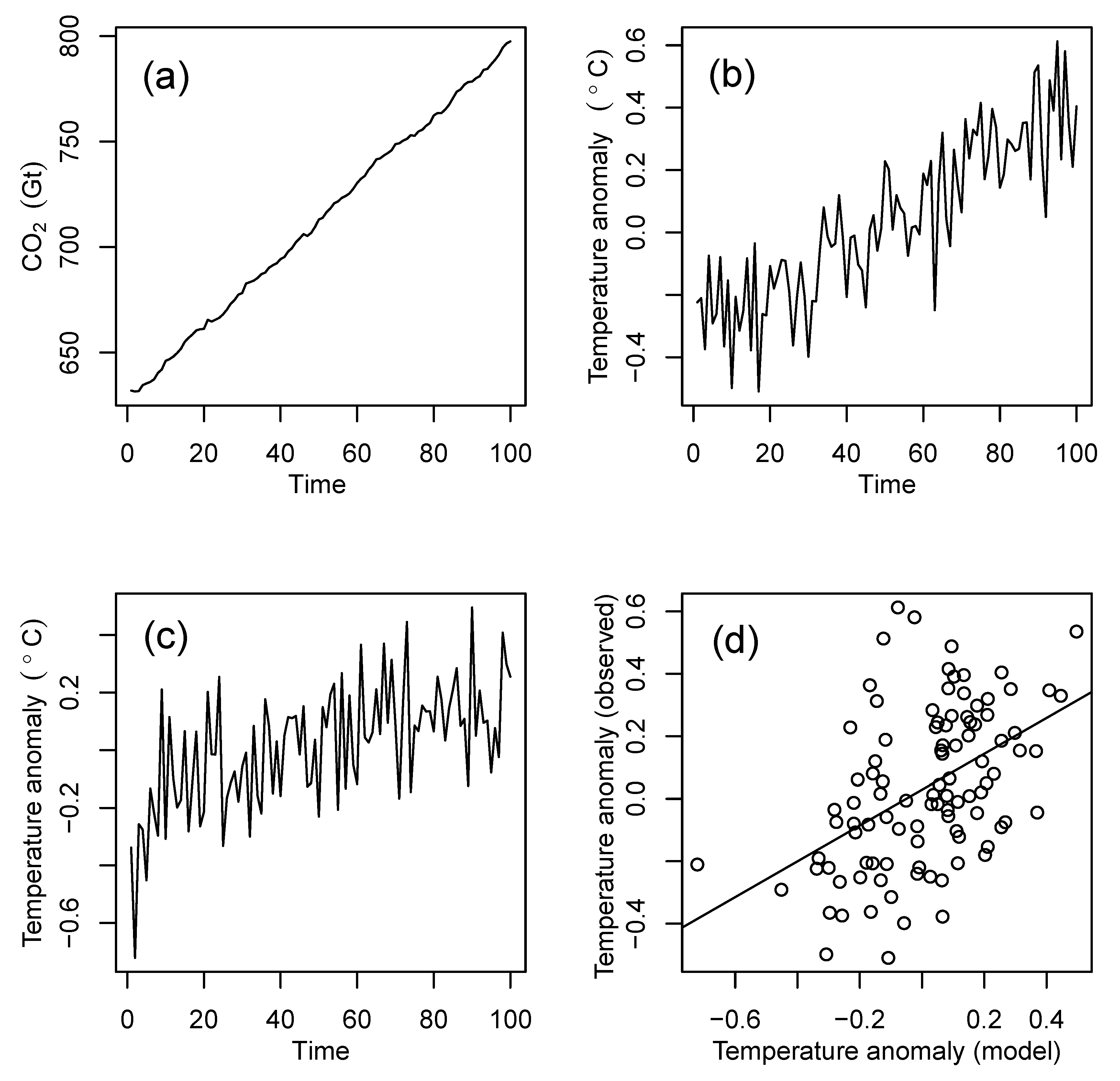
4.1. Simple Stochastic Model of the Carbon-Climate System

A simple stochastic model of the carbon–climate system can be constructed as follows. It is reasonable to assume that the observed ($y_t$) and model-simulated ($x_t$) global mean temperatures in year $t=1,2,3,\dots ,T$ are linear functions of the atmospheric carbon dioxide concentration $c_t$ [45,46] and that the carbon dioxide concentration accumulates by a random amount from year $t-1$ to year t:

$$\begin{array}{ccc}\hfill y_t& =& {\gamma }_0+{\gamma }_1{c}_t+{ϵ}_t\hfill \\ \hfill x_t& =& {\gamma }_0^{\prime }+{\gamma }_1^{\prime }{c}_t+{ϵ}_t^{\prime }\hfill \\ \hfill c_t& =& {\gamma }_c+c_{t-1}+{ϵ}_t^c,\hfill \end{array}$$

(9)

where ${\gamma }_c>0$ represents constant emissions that arrive in the atmosphere each year and ${ϵ}_t,{ϵ}_t^{\prime }$ and ${ϵ}_t^c$, are assumed to be independent Gaussian variates with zero means and constant variances. Therefore, $c_t$ is assumed to be a random-walk process with drift, which is consistent with previous studies that have shown that the time series of global mean temperature as well as the atmospheric concentration of CO${}_2$ are integrated processes of an order greater than zero [47,48,49,50,51,52]. This model is a special case of the model in Appendix A, having an instantaneous response to forcing ($\varphi ={\varphi }^{\prime }=0$). The attribution regression equation and scaling factor can be easily derived for the stochastic model. The expression for $x_t$ in Equation (9) can be used to find $c_t$, which can then be substituted into the equation for $y_t$ to give $y_t={\gamma }_0-\beta {\gamma }_0^{\prime }+\beta x_t+{ϵ}_t-\beta {ϵ}_t^{\prime }$, where the scaling factor $\beta ={\gamma }_1/{\gamma }_1^{\prime }$.

4.2. Estimation of Parameters for the Stochastic Model

Figure 5a,b show historical estimates of $c_t$ and $c_t-c_{t-1}$ using data from [53]. After 1960, when direct atmospheric measurements were available, the series $c_t-c_{t-1}$ can be seen to vary randomly around a mean of about 3 GtC/year. Before 1960, the annual changes were smoother and less variable but were then estimated from ice core data that have no annual resolution (personal communication, Prof. Pierre Friedlingstein). The sample mean and variance of the annual differences gives estimates of ${\widehat{\gamma }}_c=\overline{c_t-c_{t-1}}=1.53$ GtC/year and ${\widehat{\sigma }}_{{ϵ}^c}^2=1.43$ (GtC/year)${}^2$.

Figure 5c,d show time series plots of historical observed GMST and an example simulation from the GISS-E2-R GCM. When these are plotted against the historical CO${}_2$ values (Figure 5e,f), it can be seen that there are clear linear relationships as assumed in the stochastic model. OLS fits to these data give estimates of ${\widehat{\gamma }}_1=0.00486$ °C/GtC, ${\widehat{\gamma }}_1^{\prime }=0.00279$ °C/GtC, ${\widehat{\gamma }}_0=-3.41$ °C, ${\widehat{\gamma }}_0^{\prime }=-1.96$ °C, which gives a known scaling factor of $\beta ={\widehat{\gamma }}_1/{\widehat{\gamma }}_1^{\prime }=1.74$. The sample variance of the observed and simulated temperature residuals was similar and so for simplicity pooled sample variance was used to obtain ${\widehat{\sigma }}_{ϵ}^2={\widehat{\sigma }}_{{ϵ}^{\prime }}^2=0.0203$ (°C)${}^2$.

The stochastic model with these parameter estimates was used to simulate K = 50 independent realizations of the time series $y_t$, $x_t$, and $c_t$, where $t=1,2,\dots ,T$ years. The realizations resemble the original series, as can be seen in the $T=100$ year example shown in Figure 6.

4.3. Scaling Factor Estimates from Simulated Data

Figure 7 shows scaling factor estimates for time series of length $T=100$ years for 50 simulations from the stochastic model. The 95% prediction intervals are calculated from $\widehat{\beta }$ ± $1.96$$s_{\beta }$, where 1.96 is the 97.5th quantile of normal distribution and $s_{\beta }$ is the sample standard deviation of the 50 estimates. Figure 7a shows that the OLS estimates underestimate the true scaling factor value in all the 50 realizations. Thus the OLS estimators are strongly negatively biased. By contrast, the TLS estimates in Figure 7b appear to overestimate the scaling factor (positively biased) sometimes by a factor of two, and are a lot more variable. These results for OLS and TLS agree with the comparison made in (Van Huffel and Vandewalle [28] p. 244) for a moderate sample size—TLS estimates have a mean that is closer to the true value (i.e., are less biased) but have greater variance (i.e., are less efficient) than OLS estimates. The COINT estimates in Figure 7c are evenly scattered around the true value with a variance only slightly larger than that of the OLS estimates.

It is of interest to see how the estimates change with sample size T. Since a cointegrating relationship exists in the stochastic model ($y_t-\beta x_t$ is stationary), all the estimates should be consistent and converge on the true value as $T\to \infty$. It can be noted from Figure 8 that this appears to be the case, although for OLS (panels a and d) there is a substantial negative bias and the confidence interval does not overlap the true value even for long time series with $T=250$ years. The TLS estimates have very wide confidence intervals especially for small sample sizes $T<200$, which are typical of the sample sizes that have been used in many previous detection and attribution studies. The COINT estimates appear to be unbiased for samples with $T>50$ and the confidence intervals overlap the true value for all sample sizes. Sensitivity tests reveal that these results are robust to the choice of parameters in the stochastic model (not shown).

Figure 8 shows the accuracy of the estimators as measured by Mean Squared Error (MSE), which is the sum of the squared bias and the variance of the estimators. COINT is by far the most accurate estimator with the smallest MSE because of having small bias and small variance. For small sample sizes with $T<100$, the OLS estimator is the next most accurate estimator—despite its negative bias, it has much less variance than the TLS estimator. The TLS estimator, often used in detection and attribution studies, is the least accurate estimator of the scaling factor, primarily due to its high variance. Despite the cointegrating VAR(2) model having more parameters than the TLS regression model, it is apparent that the VAR(2) estimates have much less variance than those of TLS. This is most likely related to the problem of the TLS estimates diverging to infinity when the covariance between $y_t$ and $x_t$ is small.

5. Conclusions and Discussion

This study investigated the use of a dynamic time series model for obtaining estimates of scaling factors in detection and attribution and compared the performance to that of more traditional OLS and TLS regression approaches when applied to CMIP5 GMST simulations and simulations of a simple stochastic carbon–climate model. It has been shown that:

• The cointegrating VAR(2) model is a reasonable time series approach to use for modelling pairs of observed and model-simulated time series if one assumes the variables are AR(1) responses to common integrated forcing;
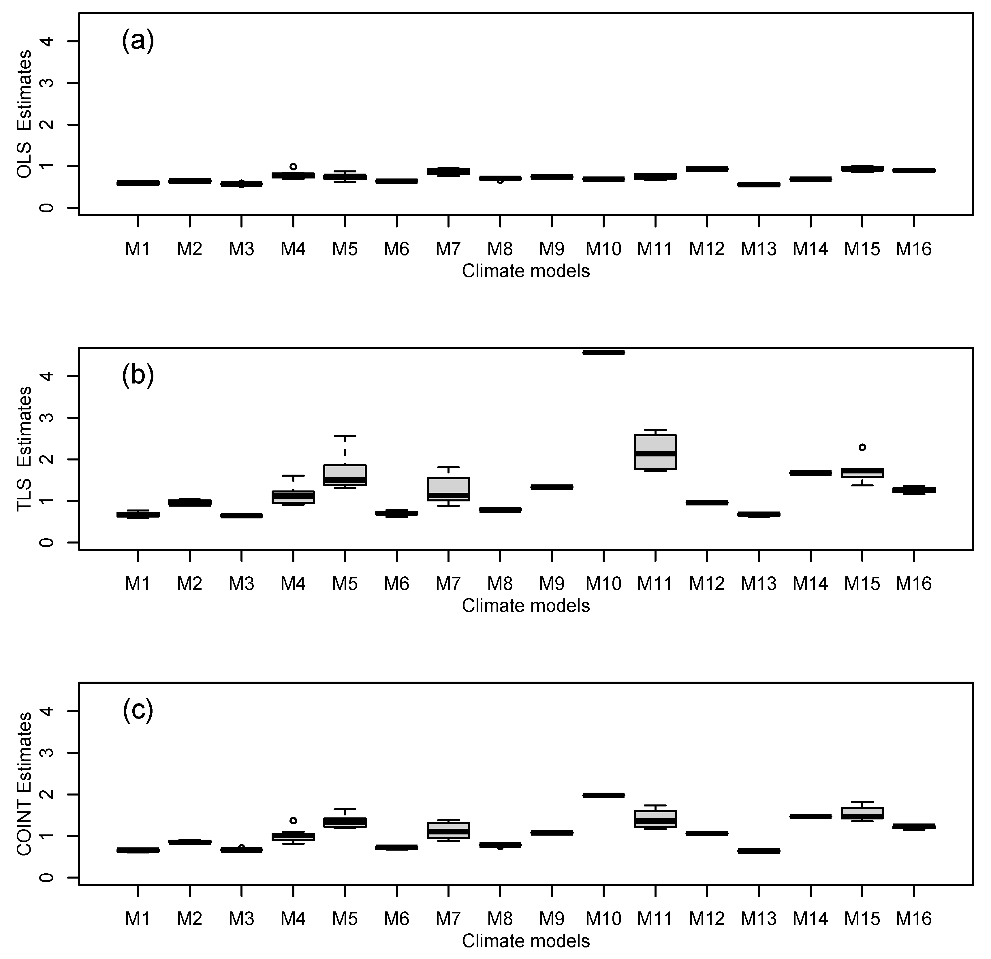
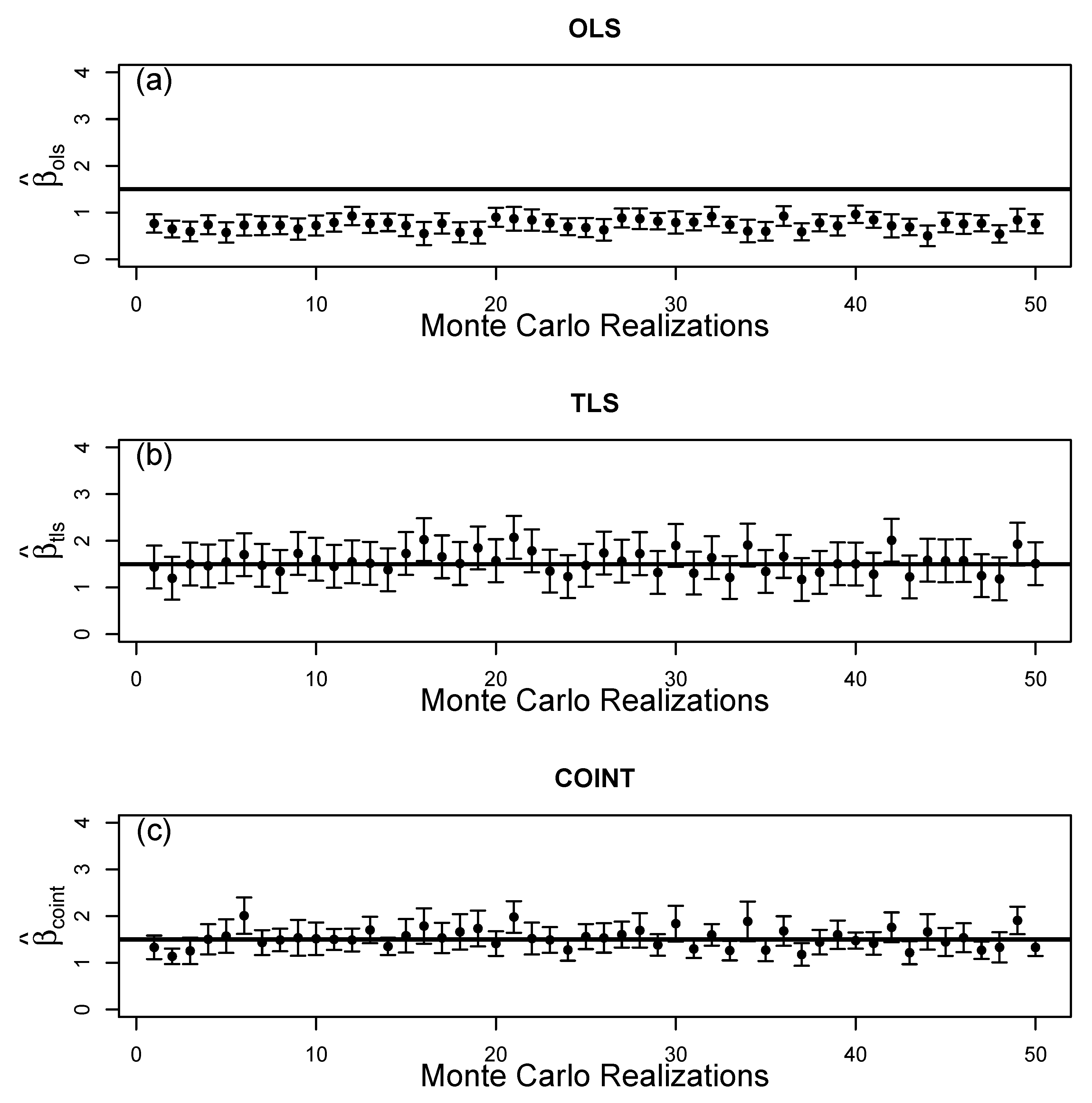
• Unlike OLS, which gives negatively biased estimates and TLS, which gives positively biased estimates (and large positive outliers), the cointegrating VAR(2) model gives estimates of the scaling factor that are unbiased;
• The cointegrating VAR(2) model estimates are much more accurate (in terms of MSE) than the OLS and TLS estimates;
• The TLS estimates have very large variance, which causes large MSE. They give infinite slope estimates if the sample covariance between the observed and model-simulated series is zero.
• Hypothesis tests on the VAR(2) fits for all the CMIP5 models reassuringly found strong evidence of a cointegrating relationship with the observations, as to be expected for observations and simulations responding to shared trending forcing.

Hence, we recommend that the cointegrated VAR(2) approach is used in future detection and attribution studies in order to obtain more reliable estimates of the scaling factor. In particular, it would be of interest to test its performance in attribution studies with more than one simulated series.

It is worth noting that the GMST response to forcing involves more than one adjustment timescale and is generally best described by a 3-box energy balance model rather than a 1-box energy balance model [17,32,54,55,56]. A vector error correction model can also be derived for this situation but results in a much less parsimonious VARMA model for the pair of observed and simulated variables. In fitting to short time series, it is advantageous to have fewer parameters to estimate, so it is likely that the VAR(2) approach remains more appropriate for most climate applications.

References

1. Haustein, K.; Allen, M.R.; Forster, P.M.; Otto, F.E.; Mitchell, D.M.; Matthews, H.D.; Frame, D.J. A real-time global warming index. Sci. Rep. 2017, 7, 15417. [Google Scholar] [CrossRef] [Green Version]
2. Sutton, R.; Suckling, E.; Hawkins, E. What does global mean temperature tell us about local climate? Philos. Trans. R. Soc. A Math. Phys. Eng. Sci. 2015, 373, 20140426. [Google Scholar] [CrossRef] [Green Version]
3. Ebi, K.L.; Åström, C.; Boyer, C.J.; Harrington, L.J.; Hess, J.J.; Honda, Y.; Kazura, E.; Stuart-Smith, R.F.; Otto, F.E. Using Detection And Attribution To Quantify How Climate Change Is Affecting Health. Health Aff. 2020, 39, 2168–2174. [Google Scholar] [CrossRef]
4. Hegerl, G.; Hoegh-Guldberg, O.; Casassa, G.; Hoerling, M.P.; Kovats, R.S.; Parmesan, C.; Pierce, D.W.; Stott, P.A. Good practice guidance paper on detection and attribution related to anthropogenic climate change. In Meeting Report of the Intergovernmental Panel on Climate Change Expert Meeting on Detection and Attribution of Anthropogenic Climate Change; 2010; Available online: https://www.ipcc.ch/publication/ipcc-expert-meeting-on-detection-and-attribution-related-to-anthropogenic-climate-change/ (accessed on 26 July 2023).
5. Allen, M.R.; Tett, S.F.B. Checking for model consistency in optimal fingerprinting. Clim. Dyn. 1999, 15, 419–434. [Google Scholar] [CrossRef] [Green Version]
6. Mitchell, J.F.B.; Karoly, D.J.; Hegerl, G.C.; Zwiers, F.W.; Allen, M.R.; Marengo, J. Detection of Climate Change and Attribution of Causes. In Climate Change 2001: The Scientific Basis. Contribution of Working Group I to the Third Assessment Report of the Intergovernmental Panel on Climate Change; Houghton, J.T., Ding, Y., Griggs, D.J., Noguer, M., Linden, P.J.v., Dai, X., Maskell, K., Johnson, C.A., Eds.; Cambridge University Press: Cambridge, UK; New York, NY, USA, 2001. [Google Scholar]
7. Hasselmann, K. Optimal fingerprints for the detection of time-dependent climate change. J. Clim. 1993, 6, 1957–1971. [Google Scholar] [CrossRef]
8. Stott, A.; Allen, M.R.; Jones, G.S. Estimating signal amplitudes in optimal fingerprinting. part II: Application to general circulation models. Clim. Dyn. 2003, 21, 493–500. [Google Scholar] [CrossRef]
9. Zhang, X.; Zwiers, F.W.; Hegerl, G.C.; Lambert, F.H.; Gillett, N.P.; Solomon, S.; Stott, P.A.; Nozawa, T. Detection of human influence on twentieth-century precipitation trends. Nature 2007, 448, 461–465. [Google Scholar] [CrossRef]
10. Allen, M.R.; Stott, P.A. Estimating signal amplitudes in optimal fingerprinting, part I: Theory. Clim. Dyn. 2003, 21, 477–491. [Google Scholar] [CrossRef]
11. Gillett, N.; Stone, D.; Stott, P.; Nozawa, T.; Karpechko, A.; Hegerl, G.; Wehner, M.; Jones, P. Attribution of polar warming to human influence. Nat. Geosci. 2008, 1, 750–754. [Google Scholar] [CrossRef] [Green Version]
12. Hegerl, G.C.; Crowley, T.J.; Allen, M.; Hyde, W.T.; Pollack, H.N.; Smerdon, J.; Zorita, E. Detection of human influence on a new, validated 1500-year temperature reconstruction. J. Clim. 2007, 20, 650–666. [Google Scholar] [CrossRef] [Green Version]
13. Hegerl, G.; Luterbacher, J.; González-Rouco, F.; Tett, S.F.B.; Crowley, T.; Xoplaki, E. Influence of human and natural forcing on european seasonal temperatures. Nat. Geosci. 2011, 4, 99–103. [Google Scholar] [CrossRef]
14. Lambert, F.; Stott, P.; Allen, M.; Palmer, M. Detection and attribution of changes in 20th century land precipitation. Geophys. Res. Lett. 2004, 31, L10203. [Google Scholar] [CrossRef]
15. Stott, P.A.; Sutton, R.T.; Smith, D.M. Detection and attribution of atlantic salinity changes. Geophys. Res. Lett. 2008, 35, L21702. [Google Scholar] [CrossRef]
16. Zwiers, F.; Zhang, X. Toward regional-scale climate change detection. J. Clim. 2003, 16, 793–797. [Google Scholar] [CrossRef]
17. Cummins, D.P.; Stephenson, D.B.; Stott, P.A. Could detection and attribution of climate change trends be spurious regression? Clim. Dyn. 2022, 59, 2785–2799. [Google Scholar] [CrossRef]
18. Hannart, A. Integrated optimal fingerprinting: Method description and illustration. J. Clim. 2016, 29, 1977–1998. [Google Scholar] [CrossRef]
19. Eyring, V.; Gillett, N.P.; Achuta Rao, K.M.; Barimalala, R.; Barreiro Parrillo, M.; Bellouin, N.; Cassou, C.; Durack, P.J.; Kosaka, Y.; McGregor, S.; et al. Human Influence on the Climate System. In Climate Change 2021: The Physical Science Basis. Contribution of Working Group I to the Sixth Assessment Report of the Intergovernmental Panel on Climate Change; Masson-Delmotte, V., Zhai, P., Pirani, A., Connors, S.L., Péan, C., Berger, S., Caud, N., Chen, Y., Goldfarb, L., Gomis, M.I., et al., Eds.; Cambridge University Press: Cambridge, UK, 2021; pp. 423–552. [Google Scholar]
20. Phillips, P.C.B. Understanding spurious regressions in econometrics. J. Econom. 1986, 33, 311–340. [Google Scholar] [CrossRef] [Green Version]
21. Granger, C.W.J.; Newbold, P. Spurious regressions in econometrics. J. Econom. 1974, 2, 111–120. [Google Scholar] [CrossRef] [Green Version]
22. Yule, G.U. Why do we sometimes get nonsense-correlations between time-series?—A study in sampling and the nature of time-series. J. R. Stat. Soc. 1926, 89, 1–63. [Google Scholar] [CrossRef]
23. Turasie, A. Cointegration Modelling of Climatic Time Series. Ph.D. Thesis, University of Exeter, Exeter, UK, 2012. Available online: https://ethos.bl.uk (accessed on 26 July 2023).
24. Juselius, K. The Cointegrated Var Model: Methodology and Applications; Oxford University Press: Oxford, UK, 2006. [Google Scholar]
25. Engle, R.F.; Granger, C.W.J. Co-integration and error correction: Representation, estimation and testing. Econometrica 1987, 55, 251–276. [Google Scholar] [CrossRef]
26. Hegerl, G.C.; von Storch, H.; Hasselmann, K.; Santer, B.D.; Cubasch, U.; Jones, P.D. Detecting Greenhouse-Gas-Induced Climate Change with an Optimal Fingerprint Method. J. Clim. 1996, 9, 2281–2306. [Google Scholar] [CrossRef]
27. Morton-Jones, A.; Henderson, R. Generalized Least Squares with Ignored Errors in Variables. Technometrics 2000, 42, 366–375. [Google Scholar] [CrossRef]
28. Van Huffel, S.; Vandewalle, J. The Total Least Squares Problem: Computational Aspects and Analysis; Society for Industrial Mathematics: Philadelphia, PA, USA, 1991. [Google Scholar]
29. Golub, G.H.; Van Loan, C.F. Matrix Computations; JHU Press: Baltimore, MA, USA, 2013. [Google Scholar]
30. Cox, P.; Huntingford, C.; Williamson, M. Emergent constraint on equilibrium climate sensitivity from global temperature variability. Nature 2018, 553, 319–322. [Google Scholar] [CrossRef] [PubMed] [Green Version]
31. Johansen, S. Estimation and hypothesis testing of cointegration vectors in gaussian vector autoregressive models. Econom. J. Econom. Soc. 1991, 59, 1551–1580. [Google Scholar] [CrossRef]
32. Cummins, D.P.; Stephenson, D.B.; Stott, P.A. Optimal Estimation of Stochastic Energy Balance Model Parameters. J. Clim. 2020, 33, 7909–7926. [Google Scholar] [CrossRef] [Green Version]
33. Beenstock, M.; Reingewertz, Y.; Paldor, N. Polynomial cointegration tests of anthropogenic impact on global warming. Earth Syst. Dyn. 2012, 3, 173–188. [Google Scholar] [CrossRef] [Green Version]
34. Estrada, F.; Perron, P. Extracting and analyzing the warming trend in global and hemispheric temperatures. J. Time Ser. Anal. 2017, 38, 711–732. [Google Scholar] [CrossRef] [Green Version]
35. Phillips, P.C.; Leirvik, T.; Storelvmo, T. Econometric estimates of earth’s transient climate sensitivity. J. Econom. 2020, 214, 6–32. [Google Scholar] [CrossRef]
36. Pretis, F. Econometric modelling of climate systems: The equivalence of energy balance models and cointegrated vector autoregressions. J. Econom. 2020, 214, 256–273. [Google Scholar] [CrossRef]
37. Stern, D.I.; Kaufmann, R.K. Anthropogenic and natural causes of climate change. Clim. Chang. 2014, 122, 257–269. [Google Scholar] [CrossRef]
38. Granger, C. Some properties of time series data and their use in econometric model specification. J. Econom. 1981, 16, 121–130. [Google Scholar] [CrossRef]
39. Johansen, S. Statistical analysis of cointegration vectors. J. Econ. Dyn. Control 1988, 12, 231–254. [Google Scholar] [CrossRef]
40. Osterwald-Lenum, M. A note with quantiles of the asymptotic distribution of the maximum likelihood cointegration rank test statistics. Oxf. Bull. Econ. Stat. 1992, 54, 461–472. [Google Scholar] [CrossRef]
41. Beenstock, M.; Reingewertz, Y.; Paldor, N. Testing the historic tracking of climate models. Int. J. Forecast. 2016, 32, 1234–1246. [Google Scholar] [CrossRef]
42. Johansen, S. Likelihood-Based Inference in Cointegrated Vector Autoregressive Models; Oxford University Press: Oxford, UK, 1995. [Google Scholar]
43. Dickey, D.A.; Fuller, W.A. Distribution of the estimators for autoregressive time series with a unit root. J. Am. Stat. Assoc. 1979, 74, 427–431. [Google Scholar]
44. Dickey, D.A.; Fuller, W.A. Likelihood ratio statistics for autoregressive time series with a unit root. Econometrica 1981, 49, 1057–1072. [Google Scholar] [CrossRef]
45. Rust, B.W.; Thijsse, B.J. Data-based models for global temperature variations. In Proceedings of the 2007 International Conference on Scientific Computing, Sozopol, Bulgaria, 5–9 June 2007; CSREA Press: Las Vegas, NV, USA, 2007; pp. 10–16. [Google Scholar]
46. Rust, B.W. A mathematical model of atmospheric retention of man-made CO2 emissions. Math. Comput. Simul. 2011, 81, 2326–2336. [Google Scholar] [CrossRef]
47. Harvey, D.I.; Mills, T.C. Modelling global temperature trends using cointegration and smooth transitions. Stat. Model. 2001, 1, 143–159. [Google Scholar] [CrossRef]
48. Kaufmann, R.K.; Stern, D.I. Cointegration analysis of hemispheric temperature relations. J. Geophys. Res. 2002, 107, 4012. [Google Scholar] [CrossRef] [Green Version]
49. Kaufmann, R.K.; Kauppi, H.; Stock, J.H. The relationship between radiative forcing and temperature: What do statistical analyses of the instrumental temperature record measure? Clim. Chang. 2006, 77, 279–289. [Google Scholar] [CrossRef] [Green Version]
50. Liu, H.; Rodríguez, G. Human activities and global warming: A cointegration analysis. Environ. Model. Softw. 2005, 20, 761–773. [Google Scholar] [CrossRef] [Green Version]
51. Stern, D.I.; Kaufmann, R.K. Econometric analysis of global climate change. Environ. Model. Softw. 1999, 14, 597–605. [Google Scholar] [CrossRef]
52. Stern, D.I.; Kaufmann, R.K. Detecting a global warming signal in hemispheric temperature series: A structural time series analysis. Clim. Chang. 2000, 47, 411–438. [Google Scholar] [CrossRef]
53. Meinshausen, M.; Vogel, E.; Nauels, A.; Lorbacher, K.; Meinshausen, N.; Etheridge, D.M.; Fraser, P.J.; Montzka, S.A.; Rayner, P.J.; Trudinger, C.M.; et al. Historical greenhouse gas concentrations for climate modelling (CMIP6). Geosci. Model. Dev. 2017, 10, 2057–2116. [Google Scholar] [CrossRef] [Green Version]
54. Caldeira, K.; Myhrvold, N.P. Projections of the pace of warming following an abrupt increase in atmospheric carbon dioxide concentration. Environ. Res. Lett. 2013, 8, 034039. [Google Scholar] [CrossRef]
55. Fredriksen, H.B.; Rypdal, M. Long-range persistence in global surface temperatures explained by linear multibox energy balance models. J. Clim. 2017, 30, 7157–7168. [Google Scholar] [CrossRef] [Green Version]
56. Tsutsui, J. Quantification of temperature response to CO2 forcing in atmosphere–ocean general circulation models. Clim. Chang. 2017, 140, 287–305. [Google Scholar] [CrossRef]
57. Pfaff, B. Analysis of Integrated and Cointegrated Time Series with R, 2nd ed.; Springer: New York, NY, USA, 2008; ISBN 0-387-27960-1. [Google Scholar]
Figure 1. Time series plots of observed (solid lines) and simulated (dashed lines) temperature anomalies for each GCM over the period 1860–2004. For simplicity, only the 1st simulation from each GCM has been shown. Temperature anomalies were calculated by subtracting the time mean over the 1960–1990 base period.
Sustainability 15 12142 g001
Figure 2. Scatter plot of observed temperature anomalies versus model simulated temperatures from the GISS-E2-R model. Best fit lines are shown for OLS regression (thin dashed lines), TLS regression (thick dashed line), and the VAR cointegrating relationship (thin solid line).
Sustainability 15 12142 g002
Figure 3. Comparison of the three estimates of the scaling factor across all 16 GCMs: (a) estimates for the first simulation from each of the 16 GCMs: O-OLS, T-TLS, and C-COINT, (b) boxplots of the scaling estimates over all simulations from each of the climate models, i.e., 70 simulated time series (see Table 1).
Sustainability 15 12142 g003
Figure 4. Boxplots of scaling factor estimates made for all available simulations of each climate model: (a) OLS estimates, (b) TLS estimates, and (c) cointegrated VAR estimates.
Sustainability 15 12142 g004
Figure 5. Time series plot of historical data over the 20th century: (a) atmospheric concentration of CO 2 (in units of Gigatons of Carbon), (b) year-to-year differences in atmospheric concentration of CO 2 , (c) observed global mean surface temperature anomalies, and (d) global mean surface temperature anomalies simulated by the GISS-E2-R model. Scatter plots of global mean temperature anomalies versus atmospheric concentration of CO 2 (with OLS fits as solid lines) for (e) observations, and (f) GISS-E2-R simulation. Temperature anomalies were calculated by subtracting the time mean over the 1960–1990 base period.
Sustainability 15 12142 g005
Figure 6. A typical example of time series simulated by the stochastic carbon–climate model: (a) atmospheric concentration of CO 2 , (b) observed temperature anomalies, (c) climate model temperature anomalies, and (d) scatter plot of observed versus simulated temperature anomalies with solid line showing the OLS fit.
Sustainability 15 12142 g006
Figure 7. Scaling factor point estimates (black circles) and 95% confidence intervals (whiskers) obtained from 50 simulations of 100-years of the carbon–climate model using (a) OLS regression, (b) TLS regression, and (c) cointegrating VAR model. The true scaling factor of 1.74 is depicted by the thick horizontal lines.
Sustainability 15 12142 g007
Figure 8. Properties of scaling factor estimates from 50 simulations of time series of lengths from 25 to 250 years. Upper panels: mean scaling factor estimates (black lines) and 95% confidence interval (grey shading) obtained by using (a) OLS regression, (b) TLS regression, and (c) cointegrating VAR. The true value of 1.74 for the scaling factor is denoted by the thick horizontal lines. Lower panels show sample properties of the estimators: (d) Mean Squared Error, (e) bias, and (f) variance.
Sustainability 15 12142 g008