Optimal Energy Consumption Path Planning for Unmanned Aerial Vehicles Based on Improved Particle Swarm Optimization

Abstract

In order to enhance the energy efficiency of unmanned aerial vehicles (UAVs) during flight operations in mountainous terrain, this research paper proposes an improved particle swarm optimization (PSO) algorithm-based optimal energy path planning method, which effectively reduces the non-essential energy consumption of UAV during the flight operations through a reasonable path planning method. First, this research designs a 3D path planning method based on the PSO optimization algorithm with the goal of achieving optimal energy consumption during UAV flight operations. Then, to overcome the limitations of the classical PSO algorithm, such as poor global search capability and susceptibility to local optimality, a parameter adaptive method based on deep deterministic policy gradient (DDPG) is introduced. This parameter adaptive method dynamically adjusts the main parameters of the PSO algorithm by monitoring the state of the particle swarm solution set. Finally, the improved PSO algorithm based on parameter adaptive improvement is applied to path planning in mountainous terrain environments, and an optimal energy-consuming path-planning algorithm for UAVs based on the improved PSO algorithm is proposed. Simulation results show that the path-planning algorithm proposed in this research effectively reduces non-essential energy consumption during UAV flight operations, especially in more complex terrain scenarios.

1. Introduction

Unmanned aerial vehicles (UAVs), controllable via onboard programming or radio remote control mechanisms, have found extensive applications in fields such as fire monitoring, target tracking, intelligent agriculture, and disaster rescue [1,2,3,4]. UAVs are typically categorized into rotary-wing UAVs and fixed-wing UAVs based on wing type, with quadrotor UAVs being the most prevalent among the rotary-wing UAVs. The preference for quadrotor UAVs stems from their advantages, like low cost, compact size, and high mobility, enabling their operation in intricate environments [5]. Despite these advantages, the ability of quadrotor UAVs to perform their tasks is often limited by their battery power consumption [6]. It is, therefore, important to investigate path-planning algorithms aimed at optimizing energy consumption without altering battery capacity in order to improve the range and efficiency of quadrotor UAVs.

In the past few years, many scholars have investigated and obtained research results on extending the life of battery storage by installing energy-harvesting devices on UAVs. In Ref. [7], the authors proposed a design of a nanoarray energy harvester based on the energy consumption model of a UAV based on the equipartitioned exciton nanoantenna technology. In Ref. [8], the authors designed an integrated energy-harvesting device that combines piezoelectric energy and solar energy. However, current related research results generally suffer from the drawbacks of high production costs and environmental impacts on the performance of energy storage devices. In contrast, from the perspective of path planning, a reasonable path-planning algorithm can reduce the non-essential energy consumption of UAVs during flight operations and then effectively improve the mission completion efficiency of UAVs. In Ref. [9], the authors derived an accurate eVTOL UAVs battery energy consumption formula based on the variation of air density with height and proposed a path applicable to complex urban environments. In Ref. [10], the authors optimized the coverage planning path of the algorithm by dividing the mission area and improved the efficiency of energy usage.

Path planning for UAVs is an integral aspect, the objective of which is to determine an optimal flight trajectory for the UAV, ensuring it avoids any obstacles and other aircraft in its surroundings [11]. Path planning techniques are essential for delineating a safe route for a UAV in a 3D space. Traditional path-planning algorithms mainly include A* algorithm [12], Dijkstra algorithm [13], Voronoi diagram [14] and the artificial potential field method [15], etc. These algorithms need to load the terrain environment information in advance, and there are the disadvantages of large computation and easy to fall into the local optimum when the terrain environment is complex. Currently, many experts use heuristic algorithms to optimize path planning and have achieved some results [16]. In Ref. [17], the authors proposed a full-coverage path-planning algorithm based on the improved genetic algorithm. In Ref. [18], the authors proposed an ant colony algorithm combined with an alert pheromone and used it for the path planning of unmanned underwater vehicles. In Ref. [19], the authors proposed a global path-planning algorithm based on an improved wolfpack algorithm for global path planning, which effectively improves the work efficiency of inspection robots. It should be noted that the tuning of the parameters in the above algorithms is completed prior to the execution of the programs and cannot be adjusted during the execution so that the algorithms cannot be adapted if the external environment change, resulting in the performance of the algorithms being compromised.

Methods for parameter tuning can generally be classified into two categories: deterministic parameter tuning and adaptive parameter tuning. Deterministic parameter tuning refers to a method where parameters are ascertained adaptively before the actual resolution of the optimization problem. Conversely, adaptive parameter tuning represents a methodology that facilitates the dynamic adaptation of algorithmic parameters during the execution of the algorithm itself [20]. Adaptive parameter tuning already exists for a wide range of applications in areas such as image processing [21] and natural language processing [22]. Significantly, in recent years, optimization algorithms based on reinforcement learning have been increasingly used for parameter tuning of heuristic algorithms and their variants. Take the PSO algorithm as an example; in the study by [23], the authors employ a Q-learning algorithm, where the strategy selected in the preceding step serves as the state input, while the selection strategy for the subsequent step is defined as the action output. The reward is then determined based on the progression of the overall optimization problem. In another study [24], the authors adopted the Q-learning algorithm, with the particle positions established as the state inputs and the anticipated velocities of different particle strategies designated as the output actions. The reward, in this case, is determined based on the augmentation or diminution of the particle evaluation value. Presently, the majority of parameter-tuning algorithms that leverage reinforcement learning are chiefly grounded in Q-learning, with adaptive control parameters and strategies. In the study [25], the authors use a strategic gradient algorithm with particle position as the state input and output action controls c1 and c2, ultimately determining the reward based on the growth rate of the overall optimization problem. Currently, parameter adaptive algorithms are mainly based on Q-learning adaptive control parameters and strategies. Compared with the Q-learning model, the deep reinforcement learning algorithm model has obvious advantages in dealing with optimization problems in continuous action space, such as parameter tuning.

In view of this, this research paper introduces a deep reinforcement learning algorithm model into the parameter adaptive algorithm, proposes an improved particle swarm algorithm based on parameter adaptation, and applies it to the optimal energy path planning for UAVs in mountainous terrain. This study provides a feasible energy-efficient path-planning method for UAVs to enhance the mission execution efficiency of UAVs in complex terrain environments. The primary contributions and innovations of this research paper can be summarized as follows:

(1)

Aiming at the problem of UAV energy waste due to unreasonable flight paths in mountainous terrain environments, this research proposes an objective cost function that integrally considers the UAV energy consumption, flight cost, terrain range and terrain collision constraints, which simplifies the optimal energy-consuming path planning problem for UAV into an objective function optimization problem based on the PSO algorithm.

(2)

In order to solve the disadvantage that the PSO algorithm easily falls into local optimum when solving complex high-dimensional problems, this research proposes an adaptive parameter control method based on the DDPG model, which effectively improves the global convergence of the PSO algorithm.

The structure of the remainder of this paper is as follows: Section 2 briefly introduces the fundamental model of the PSO algorithm, the DDPG deep reinforcement learning model, and the calculation method for the energy consumption power of the quadrotor discussed in this paper. Section 3 provides a detailed description of the proposed PSO-DDPG algorithm and its application to the path planning problem. Section 4 presents the simulation experimental environment alongside a comparative analysis with other analogous algorithms. Finally, Section 5 provides the conclusion of the paper and highlights the focus and directions for future improvement.

2. Preliminaries

In this section, some basic mathematical notation and algorithmic models are introduced.

2.1. Particle Swarm Optimization Algorithm

Particle Swarm Optimization (PSO) is a typical swarm intelligence optimization algorithm, first proposed by Dr. Kennedy and Dr. Eberhart in 1995 [26]. Particle swarm optimization combines the self-experience and social experience of particles to derive candidate solutions in the form of particles. The optimization uses a collection of flying particles in search space and moves toward a promising area to obtain a global optimal solution.

In the classical particle swarm optimization, the speed of a particle is usually affected by its previous best position and the position of the globally best particle in the swarm. To describe the state of the particle, the $i\mathrm{t}\mathrm{h}$ particle’s velocity $V_i$ and position $X_i$ are defined as follows:

$$\begin{array}{cc}{V}_i& =(v_i^1,v_i^2,\dots ,v_i^D),i=\mathrm{1,2},\dots ,N\\ X_i& =(x_i^1,x_i^2,\dots ,x_i^D),i=\mathrm{1,2},\dots ,N\end{array}$$

(1)

$D$ represents the dimension of the particle swarm search space and $N$ represents the number of particles. As the search optimization algorithm runs, the two particle movement vectors are updated as follows:

$$\begin{array}{cc}& V_i(t+1)=w{V}_i\left(t\right)+c_1\ast r_1(p{Best}_i-X_i(t\left)\right)+c_2\ast r_2(gBest-X_i(t\left)\right)\\ & X_i(t+1)=X_i\left(t\right)+V_i(t+1)\end{array}$$

(2)

$w$ is the inertia weight, $c_1$ is the cognitive acceleration coefficient, $c_2$ is the social acceleration coefficient, $r_1$ and $r_2$ are uniformly distributed random numbers within [0, 1], $V_i\left(t\right)$ represents the velocity of the $i\mathrm{t}\mathrm{h}$ particle in the $t$ generation, $p{Best}_i$ is the personal best position of the $i\mathrm{t}\mathrm{h}$ particle, and $gBest$ is the best position in the group.

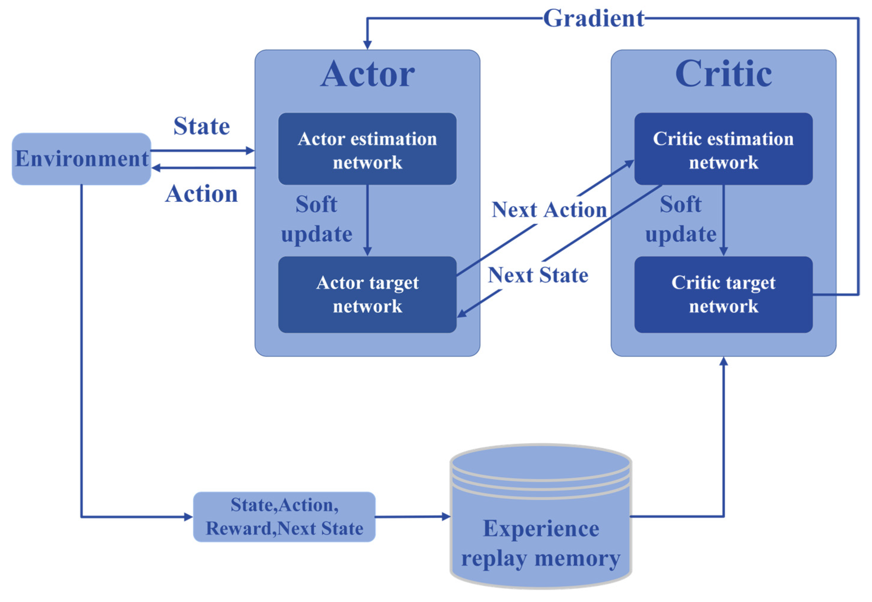
2.2. Deep Deterministic Policy Gradient

The Deep Deterministic Policy Gradient (DDPG), a variant of the deep reinforcement learning algorithm (DRL), was initially introduced by Google’s DeepMind group [27]. The DDPG algorithm can be seen as an enhanced version of the DQN algorithm with the introduction of an offline experience replay mechanism [28]. It addresses the limitations of the DQN algorithm, which struggles with continuous control problems, by employing the Actor network. Furthermore, the Critic network is utilized to evaluate the conduct of the Actor network. In DDPG, four different neural networks are considered to obtain the optimal strategy $\pi$: the Actor estimation network $\mu (s_t\mid {\theta }^{\mu })$, the Actor target network $\mathit{\mu ’}(s_t\mid {\theta }^{\mathit{\mu ’}})$, the Critic estimation network $\mathit{Q}(s_t,a_t\mid {\theta }^{\mathit{Q}})$, and the Critic target network $\mathit{Q’}(s_t,a_t\mid {\theta }^{\mathit{Q’}})$, ${\theta }^{\mu }$, ${\theta }^{\mathit{\mu ’}}$, ${\theta }^{\mathit{Q}}$ and ${\theta }^{\mathit{Q’}}$ represents the weight parameters of these neural networks.

The Actor network is designed to acquire definitive action. The Actor estimation network determines action $a_t$ based on the current state $s_t$ and generates the next state $s_{t+1}$ and reward $r_{t+1}$ by interacting with the environment. The Actor target network determines the next best action $a_{t+1}$ based on the next state $s_{t+1}$ sampled from the memory and completes the parameter update of the Critic network. The Critic network is designed to estimate the value function $\mathit{Q}$. The Critic estimation network is used to calculate the value function under the current conditions $\mathit{Q}(s_t,a_t)$. The Critic target network is used to calculate the value function in the next stage $\mathit{Q’}(s_{t+1},a_{t+1})$. To train the Critic network, we need the following minimal loss function $L$ [20]:

$$L=\frac{1}{N}\sum _i{\left(r\left(s_i,a_i\right)+\gamma \mathit{Q’}\left(s_{i+1},\mathit{\mu ’}\left(s_{i+1}∣{\theta }^{\mathit{\mu ’}}\right)∣{\theta }^{\mathit{Q’}}\right)-\mathit{Q}\left(s_i,a_i∣{\theta }^{\mathit{Q}}\right)\right)}^2$$

(3)

$\gamma$ represents the discount factor. $\gamma$ ranges from $[0,1]$.The Actor network is updated with the following policy gradient [20]:

$${{{\mathsf{\nabla }}_{{\theta }^{\mu }}J\approx \frac{1}{N}\sum _i{\mathsf{\nabla }}_a\mathit{Q}(s,a\mid {\theta }^{\mathit{Q}})|}_{s=s_i,a=\mu \left(s_i\right)}{\mathsf{\nabla }}_{{\theta }^{\mu }}\mu (s\mid {\theta }^{\mu })|}_{s_i}$$

(4)

During training, the weight parameters of these neural networks are updated as follows [20]:

$$\begin{array}{c}{\theta }^{\mathit{Q’}}\leftarrow \tau {\theta }^{\mathit{Q}}+(1-\tau ){\theta }^{\mathit{Q’}}\\ {\theta }^{\mathit{\mu ’}}\leftarrow \tau {\theta }^{\mu }+(1-\tau ){\theta }^{\mathit{\mu ’}}\end{array}$$

(5)

In the above equation, $\tau \ll 1$. The training process of DDPG is shown in Figure 1.

2.3. Calculation of the Total Output Power of the Quadcopter Battery

As a type of UAV, a quadcopter regulates the rotation speed of its rotor via four motors, thereby managing its own orientation and position. The ground coordinate system ($O_e,X_e,Y_e,Z_e$) is established based on a certain position $O_e$ on the ground, and the body coordinate system ($O_b,X_b,Y_b,Z_b$) is established based on the quadcopter frame. Figure 2 illustrates the relationship between the ground coordinate system, the body coordinate system, and the frame of the quadcopter.

Assuming the quadcopter frame is symmetrical, the center of mass aligns with the geometric center, and the impact of external resistance is disregarded, we derive the simplified quadcopter attitude dynamics model as follows [29]:

$$\begin{array}{c}\ddot{\psi }=\frac{M_x}{I_x}-\frac{(I_y-I_z)}{I_x}\dot{\theta }\dot{\phi }\\ \ddot{\theta }=\frac{M_y}{I_y}-\frac{(I_z-I_x)}{I_y}\dot{\psi }\dot{\phi }\\ \ddot{\phi }=\frac{M_z}{I_z}-\frac{(I_x-I_y)}{I_z}\dot{\theta }\dot{\psi }\end{array}$$

(6)

$I_x$, $I_y$, and $I_z$ represent the moment of inertia of quadcopter and $M_x$, $M_y$, and $M_z$ represent the attitude channel control torque of quadcopter. The streamlined model for quadcopter position dynamics can be articulated as follows [29]:

$$\begin{array}{c}\ddot{x}=(\mathrm{c}\mathrm{o}\mathrm{s}\psi \mathrm{s}\mathrm{i}\mathrm{n}\theta cos\phi +\mathrm{s}\mathrm{i}\mathrm{n}\psi \mathrm{s}\mathrm{i}\mathrm{n}\phi )\frac{F_z^b}{m}\\ \ddot{y}=(\mathrm{c}\mathrm{o}\mathrm{s}\psi \mathrm{s}\mathrm{i}\mathrm{n}\theta sin\phi -\mathrm{s}\mathrm{i}\mathrm{n}\psi \mathrm{c}\mathrm{o}\mathrm{s}\phi )\frac{F_z^b}{m}\\ \ddot{z}=\mathrm{c}\mathrm{o}\mathrm{s}\psi \mathrm{c}\mathrm{o}\mathrm{s}\theta \frac{F_z^b}{m}-g\end{array}$$

(7)

$F_z^b$ represents the pull of quadcopter, $m$ represents the takeoff weight of quadcopter, and $g$ is the acceleration due to gravity. The relationship between the quadcopter attitude channel control torque $M$ and the motor speed ${\omega }_i$ can be expressed as [29]:

$$\begin{array}{c}{F}_z^b=c_T({\omega }_1^2+{\omega }_2^2+{\omega }_3^2+{\omega }_4^2)\\ M_x=d{c}_T(\frac{\sqrt{2}}{2}{\omega }_1^2-\frac{\sqrt{2}}{2}{\omega }_2^2-\frac{\sqrt{2}}{2}{\omega }_3^2+\frac{\sqrt{2}}{2}{\omega }_4^2)\\ M_y=d{c}_T(\frac{\sqrt{2}}{2}{\omega }_1^2+\frac{\sqrt{2}}{2}{\omega }_2^2-\frac{\sqrt{2}}{2}{\omega }_3^2-\frac{\sqrt{2}}{2}{\omega }_4^2)\\ M_z=c_M({\omega }_1^2-{\omega }_2^2+{\omega }_3^2-{\omega }_4^2)\end{array}$$

(8)

$d$ represents the distance from the center of the quadcopter body to a certain motor, and is taken as $0.4\mathrm{m}$, $c_T$ is the tensile coefficient of the propeller with a value of $1.55\times {10}^{-4}$, and $c_M$ represents the torque coefficient of the propeller with a value of $4.11\times {10}^{-6}$.

The total output power $P_T$ of the quadcopter battery can be determined using the following equation [30]:

$$P_T=\sum _{i=1}^4\left(U_{mi}+I_{m_i}{R}_e\right)I_{m_i}$$

(9)

$U_{mi}$, $I_{m_i}$, and $R_e$ represent the equivalent voltage, equivalent current, and armature internal resistance of the UAV motor, respectively. Equivalent voltage $U_m$ and Equivalent current $I_m$ of each motor are configured according to the following equation [30]:

$$\begin{array}{c}{U}_m=(\frac{M{K}_{v_0}{U}_{m_0}}{9.55(U_{m_0}-I_{m_0}{R}_e)}+U_{m_0})+\frac{U_{m_0}-I_{m_0}{R}_e}{K_{v_0}{U}_{m_0}}N\\ I_m=\frac{M{K}_{v_0}{U}_{m_0}}{9.55(U_{m_0}-I_{m_0}{R}_e)}{I}_{m_0}\end{array}$$

(10)

$U_{m_0}$ represents the nominal no-load voltage, $I_{m_0}$ is the nominal no-load current, $K_{v_0}$ represents the motor KV value, $M$ denotes the motor load torque, and $N$ represents the motor speed. In this study, $U_{m_0}$ is taken as 22.2, $I_{m_0}$ is taken as 1.1 and $K_{v_0}$ is taken as 170. $N$ can be calculated from the angular velocity of the motor ${\omega }_i$, and $M$ can be calculated using the following equation [30]:

$$M=C_m\rho {\left(\frac{N}{60}\right)}^2{D}_p^5$$

(11)

$\rho$ represents the air density in the current working environment of the UAV with a value of $1.293\mathrm{k}\mathrm{g}/{\mathrm{m}}^3$, $D_p$ represents the diameter of the quadcopter propeller with a value of $0.508$, and $C_m$ represents the total torque coefficient with a value of $0.0031$. In the numerical simulation experiments of this study, the relevant parameters are generated in ”https://flyeval.com (accessed on 6 July 2023)”.

3. Optimal Energy Consumption Path Planning Based on PSO-DDPG

In this section, we design an adaptive parameter control methodology rooted in the DDPG deep reinforcement learning model and combine this algorithm with the PSO algorithm to propose an optimal energy consumption UAV path-planning algorithm.

3.1. Problem Modelling

3.1.1. Environmental Model

In three-dimensional flight space, the results of UAV path planning can often be described via a discrete set of waypoints $\{p_0,p_1,p_2,\dots ,p_n,p_{n+1}\}$; the first waypoint $p_0$ is the starting point and the last waypoint $p_{n+1}$ is the target point, and the coordinate of $p_i$ is $(x_i,y_i,z_i)$. In this algorithm, every waypoint is regarded as a particle within the MOPSO algorithm. In scenarios with multiple UAVs involved in the mission, the routing of the UAVs is determined based on their priority within the formation. To deter frequent angle changes during the flight, which could compromise flight safety, a cubic B-spline curve is utilized to smooth the flight route [31].

The 3D map environment information, which is necessary for UAV path planning, must be derived from the terrain model. Effective terrain modeling can substantially enhance the accuracy of the path-planning algorithm. In this paper, considering obstacles, environment, and other factors, the following valley terrain model was established [32]:

$$Z_2(x,y)=\sum _{i=1}^n{h}_i\mathrm{e}\mathrm{x}\mathrm{p}[-{\left(\frac{x-x_{mi}}{x_{si}}\right)}^2-{\left(\frac{y-y_{mi}}{y_{si}}\right)}^2]$$

(12)

where $(x_{mi},y_{mi})$ is the central coordinate of the i-th peak; $h_i$ is a topographic parameter that controls the height of the peak, $x_{si}$ and $y_{si}$ are the attenuation of the $i^{th}$ peak along the x- and y-axes, which control the slope of the peak, $n$ represents the total number of peaks. The unobstructed regions within the 3D map can be considered as the solution space for the path planning issue.

3.1.2. Basic PSO Design for Path Planning

The evaluation objective function (fitness function) of UAV path planning includes the energy consumption cost function $F_1$, the distance cost function $F_2$ and the constraint cost function $F_3$, and the mathematical expression of the fitness function is:

$$Fitness=k_1{F}_1+k_2{F}_2+k_3{F}_3$$

(13)

The energy cost function $F_1$ can be given as follows:

$$F_1=0.0001\ast \sum _{i=1}^n{P}_T^i$$

(14)

where $P_T^i$ represents the battery energy consumption power obtained by the ith path point obtained after spline interpolation, $k_1$ is the energy cost factor, and $k_1=1$in this algorithm. The distance cost function $F_2$ can be expressed as follows:

$$F_2=\sum _{i=1}^{n-1}\sqrt{{(x_{i+1}-x_i)}^2+{(y_{i+1}-y_i)}^2+{(z_{i+1}-z_i)}^2}$$

(15)

where ${(x}_i{,y}_i,z_i)$ are the $i\mathrm{t}\mathrm{h}$ path point of the planned path. $k_2$ is the path cost factor, $k_2=1$in this algorithm. The constraint cost function $F_3$ can be expressed as follows:

$$F_3=F_1+F_2$$

(16)

$k_3$ is the collision penalty factor. If the planned path interferes with the terrain or exceeds the boundaries, $k_3=1000$; otherwise, $k_3=0$.

3.2. DDPG-Based Parameter Adaptation Method for PSO Algorithm

3.2.1. State Space

The state space, serving as the input for the Actor network, dictates the convergence rate of the algorithm. For conventional deep reinforcement learning methods, the state space design should satisfy the following criteria:

• The chosen states should have relevance to the task objective;
• The chosen states should be as mutually independent as possible and encompass all task indicators;
• The chosen states should be capable of mapping to the same value range.

Adhering to the aforementioned principles, the state space of the algorithm comprises three elements: the evolutionary progress of the population, the population diversity, and the present optimization capability of the population.

The iteration percentage in particle swarm optimization is a parameter that signifies the extent of algorithm execution. At the algorithm’s commencement, this iteration progress is at 0%, incrementally increasing until the algorithm’s completion, at which point it reaches 100%. The definition of the iteration percentage can be formulated using the following equation:

$$Iter=N_{now}/N_{max}$$

(17)

where $N_{now}$ is the current number of iterations of the particle swarm and $N_{max}$ is the maximum number of iterations of the particle swarm.

The diversity of the particle swarm, which signifies the degree of variation among particle populations, is formulated as per the equation below:

$$Div=\frac{1}{M}\sum _{i=1}^M\sqrt{\sum _{j=1}^3{\left[{\mathit{q}}_{ij}-\overline{{\mathit{q}}_j}\right]}^2/\sum _{j=1}^3{\left[{\mathit{q}}_j^{max}-\overline{{\mathit{q}}_j}\right]}^2}$$

(18)

where $M$ is the number of particles in the swarm, and ${\mathit{q}}_{ij}$ is the jth position of the ith particle. $\overline{{\mathit{q}}_j}$ is the mean value of the swarm at the $j\mathrm{t}\mathrm{h}$ position, ${\mathit{q}}_j^{max}$ and ${\mathit{q}}_j^{min}$ are the maximum and minimum values of the swarm at the $j\mathrm{t}\mathrm{h}$ position.

The current optimization capabilities of the particle swarm, a measure that reflects the extent of the particle swarm’s evolution relative to the previous generation, is determined using the subsequent equation:

$$Evo=\sqrt{\sum _{k=1}^3{\left(F_k^{gbest}\right(t-1)-F_k^{gbest}(t\left)\right)}^2/\sum _{k=1}^3{\left(F_k^{gbest}\right(t-1\left)\right)}^2}$$

(19)

where $F_k^{gbest}\left(t\right)$ is the $k\mathrm{t}\mathrm{h}$ fitness function value of the global optimal solution selected at moment $t$.

3.2.2. Action Space

Action constitutes the output of the Actor network, serving to produce parameters for each iteration of the PSO optimization algorithm. In this algorithm, we define the continuous action $a$ as an array $\left(a1,a2,a3\right)$ and the values of $w$, $c1$ and $c2$ are designed according to the following equations:

$$\begin{array}{c}w=a1+w_{last}\\ c1=a2+c{1}_{last}\\ c2=a3+c{2}_{last}\end{array}$$

(20)

where $w_{last}$, ${c1}_{last}$, ${c2}_{last}$ are the parameters of previous round of the PSO optimization algorithm.

3.2.3. Reward Function

The reward function’s purpose is to compute the rewards obtained by ‘Action’ within the task environment. Within this algorithm, the reward function is devised based on the ensuing equations, thereby propelling the PSO algorithm toward an optimal global solution:

$$r\left(t\right)=\left\{\begin{array}{c}-1, g\mathrm{Best}(t+1)=g\mathrm{Best}\left(t\right)\\ 1, g\mathrm{Best}(t+1)<g\mathrm{Best}\left(t\right)\end{array}\right.$$

(21)

3.3. PSO-DDPG for Path Planning

In this subsection, the enhanced PSO algorithm is applied to address the problem of optimal energy consumption path planning for UAVs in complex terrain environments. This application is based on the deep reinforcement learning adaptive parameter model proposed in this study. The augmented algorithm’s implementation aligns with the framework depicted in Algorithm 1, while the algorithm’s crucial parameters are presented in

Table 1. Main parameters designed in the algorithm.

Quantity	Symbol	Value
Number of total group	M	50
Number of total iterations	N	100
Current particle number	i	\
Current iterations	t	\
Number of iterations to reach the neural network learning condition	$t_{learn}$	\
Number of path points	n	1000
Capacity of experience replay memory	R	10
Inertia weight	$w$	0.4~2.0
Social weight	$c1$	0.8~2.0
Cognitive weight	$c2$	0.8~2.0
Discount factor	$\gamma$	0.95

.

Algorithm 1 PSO-DDPG based 3D environment UAV path planning

1: Initialize the three-dimension environment information 2: Initialize the number of population particles M, the maximum number of iterations N and the initial parameters $(w,c1,c2)$ 3: for i = 1: M 4:   Initialize the particle location $X_i$ and velocities $V_i$ 5: end for 6: Randomly initialize critic and actor network with weights ${\theta }^{\mu }$ and ${\theta }^{\mathit{Q}}$ 7: Initialize target network with weights ${\theta }^{\mathit{\mu ’}}\leftarrow {\theta }^{\mu }$ and ${\theta }^{\mathit{Q’}}\leftarrow {\theta }^{\mathit{Q}}$ 8: Initialize the experience replay memory R 9: for t = 1: N 10:  Obtain the state $s_t$ from the environment 11:  Input $s_t$ into the actor estimation network to obtain the action $a_t$ 12:  Calculate the parameters $w$, $c1$ and $c2$ 13:  for i = 1: M 14:   Update the particle location $X_i$ and velocities $V_i$ 15:  end for 16:  Calculate the reward $r$ and the next state $s_{t+1}$ 17:  Save $(s_t,a_t,r,s_{t+1})$ to the experience replay memory R 18:  Extract data from experience replay memory R and update ${\theta }^{\mu }$ and ${\theta }^{\mathit{Q}}$ 19:  Update critic and actor network with weights ${\theta }^{\mu }$ and ${\theta }^{\mathit{Q}}$ 20:  if t = $t_{learn}$ 21:   Initialize target network with weights ${\theta }^{\mathit{Q’}}\leftarrow \tau {\theta }^{\mathit{Q}}+(1-\tau ){\theta }^{\mathit{Q’}}$ and ${\theta }^{\mathit{\mu ’}}\leftarrow \tau {\theta }^{\mu }+(1-\tau ){\theta }^{\mathit{\mu ’}}$ 22:  end if 23: end for

4. Simulation Analysis and Discussion

This section begins with an overview of the task scenario setup and the experimental hardware configuration for the numerical simulations. Subsequently, numerical simulations are carried out for different initial values of parameters and different task scenarios, respectively. Through a comparative analysis of the simulation results, the superior performance of the PSO-DDPG algorithm proposed in this study is demonstrated compared to other similar algorithms.

4.1. Experimental Environment

To assess the performance of the algorithm proposed in this study, two sets of numerical simulation experiments were carried out. The Environmental Model employed for these simulations is a 100 × 100 × 100 3D space, with obstacles generated using the mountain model function described in Section 3.1.1, as depicted in Figure 3.

It is important to note that the numerical simulations in this study were conducted using the MATLAB R2021a simulation platform on a Windows 10 64-bit system.

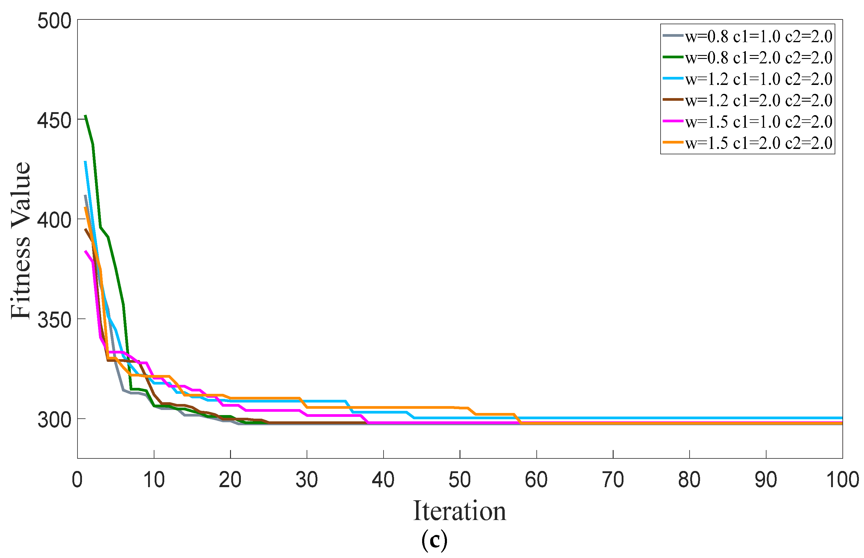
4.2. Case 1: Comparative Analysis under the Different Initial Values of Parameters

To assess the performance of the algorithms under different initial values of parameters, this section presents numerical simulations of the classical PSO algorithm, the reinforcement learning-based parameter adaptation algorithm (RLPSO) and the PSO-DDPG algorithm proposed in this paper in a simulation scenario. To ensure the validity of the simulation results, the parameter settings of the three algorithms are referred to in Table 1. This group of simulation experiments uses a 3D simulation terrain, as shown in Figure 3, the starting point of the UAV path planning is (1, 1, 1), and the endpoint is (100, 100, 30). Each algorithm is initialized by the same six sets of parameters. The initial values for each parameter group are indicated in the legend.

Figure 4 shows the global convergence solution for the worst-performing set of initial parameters in each algorithm. Figure 5 shows the convergence curves of optimal fitness values for each algorithm for different values of the initial parameters. As can be seen from the figures, the performance of the classical PSO algorithm is sensitive to different initial values of the parameters, and inappropriate initial parameters can lead the algorithm to converge to a poor global optimal solution. The RLPSO optimization algorithm has been optimized in terms of both parameter adaptation and global convergence, but its global convergence value still has the potential to be improved. Compared with other algorithms, the PSO-DDPG optimization algorithm proposed in this paper performs well in terms of parameter adaptation and shows good global convergence even when the initial values of the parameters are not set properly.

4.3. Case 2: Simulation Analysis in Different Terrain Environments

To assess the performance of the algorithm in terrain environments of varying complexity, this subsection sets up two different terrain scenarios, simple and complex, depending on the number of obstacle peaks. We have carried out numerical simulations using the classical PSO algorithm, the Artificial Bee Colony algorithm (ABC) [33] and the Artificial Fish Swarm algorithm (AFSA) [34] as reference groups. The parameter settings for each test algorithm are shown in

Table 2. Parameter settings of the different test algorithms. (meaning of the symbols are provided in the respective pieces of literature).

Algorithm	Parameter
PSO	$w=0.8$, $c1=c2=2.0$, $V_{\mathrm{m}\mathrm{a}\mathrm{x}}=0.1\times \mathrm{R}\mathrm{a}\mathrm{n}\mathrm{g}\mathrm{e}$
ABC	$n_{onlook}=10$, $\phi =1.2$, $P=0.5$, $V_{\mathrm{m}\mathrm{a}\mathrm{x}}=0.1\times \mathrm{R}\mathrm{a}\mathrm{n}\mathrm{g}\mathrm{e}$
AFSA	$Visual=0.5\times \mathrm{R}\mathrm{a}\mathrm{n}\mathrm{g}\mathrm{e}$, $Step=0.1\times \mathrm{R}\mathrm{a}\mathrm{n}\mathrm{g}\mathrm{e}$, $\delta =10$

.

Figure 6 displays the optimal flight paths generated by different algorithms in a simple terrain environment, while Figure 7 illustrates the target cost function curves obtained by these algorithms in the same environment. From Figure 6 and Figure 7, it can be seen that in a simple terrain environment, the classical PSO algorithm and the ABC algorithm fall into local optimization, the AFSA algorithm performs better in terms of global convergence but shows a long convergence time due to its high complexity, and the PSO-DDPG algorithm proposed in this paper performs optimally in terms of overall performance.

Figure 8 and Figure 9 show the fly optimal flight path and target cost function curves for different algorithms in complex terrain environments. As can be seen in Figure 8 and Figure 9, the classical PSO and ABC algorithms show an exacerbation of the local optimum problem as the number of peaks in the terrain environment increases, while the problem of slower convergence of the AFSA algorithm remains. On the contrary, although the PSO-DDPG algorithm proposed in this paper decreases in convergence speed, its comprehensive performance is still the best among similar algorithms.

Table 3. Simulation result statistics for each algorithm in simple terrain.

Algorithm	Average Fitness Value	Best Fitness Value	Worst Fitness Value	Average Optimization Rates
PSO	323.592	322.76	325.59	\
ABC	305.518	304.91	307.25	0.056
AFSA	299.77	298.13	301.47	0.074
PSO-DDPG	299.47	295.36	301.48	0.075

and

Table 4. Simulation result statistics for each algorithm in complex terrain.

Algorithm	Average Fitness Value	Best Fitness Value	Worst Fitness Value	Average Optimization Rates
PSO	334.39	334.48	338.36	\
ABC	324.03	318.19	327.45	0.031
AFSA	306.66	306.17	307.21	0.083
PSO-DDPG	303.84	301.35	306.01	0.092

present the simulation results and optimization ratio of each algorithm compared to the classical PSO algorithm, which was obtained from ten simulations of the four algorithms. Comparing Table 3 and Table 4, the classical PSO algorithm and the ABC optimization algorithm show poor global convergence in both simple and complex terrain environments, and the AFSA optimization algorithm shows better convergence in simple terrain, but the global convergence is affected in complex terrain. The PSO-DDPG algorithm proposed in this paper performs optimally in terms of global convergence.

5. Conclusions

This research introduces an enhanced PSO path-planning algorithm that employs a parametric adaptive approach for achieving optimal energy consumption path planning of quadrotors in valley terrain environments. Firstly, the UAV optimal energy consumption path planning problem is formulated as an objective function optimization problem with constraints, including collision threats and area restrictions. The classical PSO algorithm is utilized to solve the objective function optimally. Secondly, to address the lack of adaptability and susceptibility to local optima in the classical PSO algorithm, we introduce a deep deterministic policy gradient (DDPG) model. This model adaptively adjusts the three parameters $w$, $c1$ and $c2$ in the PSO algorithm during its operation, thereby enhancing the algorithm’s search performance. The numerical simulations conducted in a 3D environment with other similar algorithms demonstrate the advantageous performance of the proposed algorithm in this paper. Compared to the classical PSO algorithm, the PSO-DDPG algorithm proposed in this paper achieves optimization rates of 7.5% and 9.2% in simple and multi-peaked complex terrain, respectively.

In this study, a path-planning algorithm for UAVs is proposed with the objective of optimal energy consumption in a mountainous terrain environment, and the effectiveness of the proposed algorithm and its performance advantage over similar algorithms are verified through scenario simulation. Nevertheless, this study does not consider the impact of environmental factors on UAV energy consumption; for example, in a wind field, strong gusts of wind will cause the UAV to generate greater energy consumption, which is due to the need for the UAV to maintain attitude stability in the wind field. In future work, we will consider the effect of such factors on UAV energy consumption, further improve the energy consumption calculation model for UAVs, and try to deploy the algorithm to real UAVs to provide effective control decisions for flight operations in real environments.

References

1. De Vivo, F.; Battipede, M.; Johnson, E. Infra-red line camera data-driven edge detector in UAV forest fire monitoring. Aerosp. Sci. Technol. 2021, 111, 106574. [Google Scholar] [CrossRef]
2. Altan, A.; Hacıoğlu, R. Model predictive control of three-axis gimbal system mounted on UAV for real-time target tracking under external disturbances. Mech. Syst. Signal Process. 2020, 138, 106548. [Google Scholar] [CrossRef]
3. Shahi, T.B.; Xu, C.-Y.; Neupane, A.; Guo, W. Recent Advances in Crop Disease Detection Using UAV and Deep Learning Techniques. Remote Sens. 2023, 15, 2450. [Google Scholar] [CrossRef]
4. Silvagni, M.; Tonoli, A.; Zenerino, E.; Chiaberge, M. Multipurpose UAV for search and rescue operations in mountain avalanche events. Geomat. Nat. Hazards Risk 2017, 8, 18–33. [Google Scholar] [CrossRef] [Green Version]
5. Lozano, Y.; Gutiérrez, O. Design and Control of a Four-Rotary-Wing Aircraft. IEEE Lat. Am. Trans. 2016, 14, 4433–4438. [Google Scholar] [CrossRef]
6. Belge, E.; Altan, A.; Hacıoğlu, R. Metaheuristic Optimization-Based Path Planning and Tracking of Quadcopter for Payload Hold-Release Mission. Electronics 2022, 11, 1208. [Google Scholar] [CrossRef]
7. Citroni, R.; Di Paolo, F.; Livreri, P. A Novel Energy Harvester for Powering Small UAVs: Performance Analysis, Model Validation and Flight Results. Sensors 2019, 19, 1771. [Google Scholar] [CrossRef] [Green Version]
8. Wang, Y.; Kumar, L.; Raja, V.; Al-bonsrulah, H.A.Z.; Kulandaiyappan, N.K.; Amirtharaj Tharmendra, A.; Marimuthu, N.; Al-Bahrani, M. Design and Innovative Integrated Engineering Approaches Based Investigation of Hybrid Renewable Energized Drone for Long Endurance Applications. Sustainability 2022, 14, 16173. [Google Scholar] [CrossRef]
9. Li, Y.; Liu, M. Path Planning of Electric VTOL UAV Considering Minimum Energy Consumption in Urban Areas. Sustainability 2022, 14, 13421. [Google Scholar] [CrossRef]
10. Baras, N.; Dasygenis, M. UGV Coverage Path Planning: An Energy-Efficient Approach through Turn Reduction. Electronics 2023, 12, 2959. [Google Scholar] [CrossRef]
11. Zhang, X.; Duan, H. An improved constrained differential evolution algorithm for unmanned aerial vehicle global route planning. Appl. Soft Comput. 2015, 26, 270–284. [Google Scholar] [CrossRef]
12. Bayili, S.; Polat, F. Limited-Damage A*: A path search algorithm that considers damage as a feasibility criterion. Knowl.-Based Syst. 2011, 24, 501–512. [Google Scholar] [CrossRef]
13. Dijkstra, E.W. A note on two problems in connexion with graphs. Numer. Math. 1959, 1, 269–271. [Google Scholar] [CrossRef] [Green Version]
14. Pehlivanoglu, Y.V. A new vibrational genetic algorithm enhanced with a Voronoi diagram for path planning of autonomous UAV. Aerosp. Sci. Technol. 2012, 16, 47–55. [Google Scholar] [CrossRef]
15. Xie, S.; Hu, J.; Bhowmick, P.; Ding, Z.; Arvin, F. Distributed Motion Planning for Safe Autonomous Vehicle Overtaking via Artificial Potential Field. IEEE Trans. Intell. Transp. Syst. 2022, 23, 21531–21547. [Google Scholar] [CrossRef]
16. Wen, J.; Yang, J.; Wang, T. Path Planning for Autonomous Underwater Vehicles Under the Influence of Ocean Currents Based on a Fusion Heuristic Algorithm. IEEE Trans. Veh. Technol. 2021, 70, 8529–8544. [Google Scholar] [CrossRef]
17. Wu, X.; Bai, J.; Hao, F.; Cheng, G.; Tang, Y.; Li, X. Field Complete Coverage Path Planning Based on Improved Genetic Algorithm for Transplanting Robot. Machines 2023, 11, 659. [Google Scholar] [CrossRef]
18. Ma, Y.N.; Gong, Y.J.; Xiao, C.F.; Gao, Y.; Zhang, J. Path Planning for Autonomous Underwater Vehicles: An Ant Colony Algorithm Incorporating Alarm Pheromone. IEEE Trans. Veh. Technol. 2019, 68, 141–154. [Google Scholar] [CrossRef]
19. Wang, Z.; Yu, R.; Yang, T.; Xu, J.; Meng, Y. Robot navigation path planning in power plant based on improved wolf pack algorithm. In Proceedings of the 2021 4th International Conference on Information Systems and Computer Aided Education 2021, Dalian China, 24–26 September 2021; pp. 2824–2829. [Google Scholar]
20. Yin, S.; Jin, M.; Lu, H.; Gong, G.; Mao, W.; Chen, G.; Li, W. Reinforcement-learning-based parameter adaptation method for particle swarm optimization. Complex Intell. Syst. 2023. [Google Scholar] [CrossRef]
21. Liu, Z.; Lin, Y.; Cao, Y.; Hu, H.; Wei, Y.; Zhang, Z.; Lin, S.; Guo, B. Swin Transformer: Hierarchical Vision Transformer using Shifted Windows. In Proceedings of the 2021 IEEE/CVF International Conference on Computer Vision (ICCV), Montreal, BC, Canada, 10–17 October 2021; pp. 9992–10002. [Google Scholar]
22. Shi, Y.; Eberhart, R. A modified particle swarm optimizer. In Proceedings of the 1998 IEEE International Conference on Evolutionary Computation Proceedings. IEEE World Congress on Computational Intelligence (Cat. No.98TH8360), Anchorage, AK, USA, 4–9 May 1998; pp. 69–73. [Google Scholar]
23. Liu, Y.; Lu, H.; Cheng, S.; Shi, Y. An Adaptive Online Parameter Control Algorithm for Particle Swarm Optimization Based on Reinforcement Learning. In Proceedings of the 2019 IEEE Congress on Evolutionary Computation (CEC), Wellington, New Zealand, 10–13 June 2019; pp. 815–822. [Google Scholar]
24. Lillicrap, T.P.; Hunt, J.J.; Pritzel, A.; Heess, N.M.O.; Erez, T.; Tassa, Y.; Silver, D.; Wierstra, D.J.C. Continuous control with deep reinforcement learning. arXiv 2015, arXiv:1509.02971. [Google Scholar]
25. Wu, D.; Wang, G.G. Employing reinforcement learning to enhance particle swarm optimization methods. Eng. Optim. 2022, 54, 329–348. [Google Scholar] [CrossRef]
26. Kennedy, J.; Eberhart, R. Particle swarm optimization. In Proceedings of the ICNN’95-International Conference on Neural Networks, Perth, WA, Australia, 27 November–1 December 1995; Volume 1944, pp. 1942–1948. [Google Scholar]
27. Silver, D.; Lever, G.; Heess, N.; Degris, T.; Wierstra, D.; Riedmiller, M. Deterministic policy gradient algorithms. In Proceedings of the 31st International Conference on International Conference on Machine Learning, Beijing, China, 21–26 June 2014; Volume 32, pp. I–387–I–395. [Google Scholar]
28. Schaul, T.; Quan, J.; Antonoglou, I.; Silver, D. Prioritized Experience Replay. arXiv 2015, arXiv:1511.05952. [Google Scholar]
29. Thu, K.M.; Gavrilov, A.I. Designing and Modeling of Quadcopter Control System Using L1 Adaptive Control. Procedia Comput. Sci. 2017, 103, 528–535. [Google Scholar] [CrossRef]
30. Shi, D.; Dai, X.; Zhang, X.; Quan, Q. A Practical Performance Evaluation Method for Electric Multicopters. IEEE/ASME Trans. Mechatron. 2017, 22, 1337–1348. [Google Scholar] [CrossRef]
31. Song, B.; Wang, Z.; Zou, L. An improved PSO algorithm for smooth path planning of mobile robots using continuous high-degree Bezier curve. Appl. Soft Comput. 2021, 100, 106960. [Google Scholar] [CrossRef]
32. Xia, L.; Jun, X.; Manyi, C.; Ming, X.; Zhike, W. Path planning for UAV based on improved heuristic A* algorithm. In Proceedings of the 2009 9th International Conference on Electronic Measurement & Instruments, Beijing, China, 16–19 August 2009; pp. 3-488–3-493. [Google Scholar]
33. Karaboga, D. An Idea Based on Honey Bee Swarm for Numerical Optimization, Technical Report-TR06; Erciyes University: Talas, Turkey, 2005. [Google Scholar]
34. Zhang, Y.; Guan, G.; Pu, X. The Robot Path Planning Based on Improved Artificial Fish Swarm Algorithm. Math. Probl. Eng. 2016, 2016, 3297585. [Google Scholar] [CrossRef] [Green Version]
Figure 1. Training process of deep deterministic policy gradient (DDPG).
Sustainability 15 12101 g001
Figure 2. Simplified schematic of the quadrotor. ω i represents the angular velocity of each motor of the quadcopter, ψ , θ , and φ represent the pitch angle, roll angle, and yaw angle of the quadcopter, respectively.
Sustainability 15 12101 g002
Figure 3. Example of a simulation scenario in this article.
Sustainability 15 12101 g003
Figure 4. Global convergence solution for the worst-performing set of initial parameters based on different algorithms.
Sustainability 15 12101 g004
Figure 5. Convergence curves of optimal fitness values based on different algorithms in Case 1 (a) PSO (b) RLPSO (c) PSO-DDPG.
Sustainability 15 12101 g005aSustainability 15 12101 g005b
Figure 6. Optimal flight paths for different algorithms in simple terrain.
Sustainability 15 12101 g006
Figure 7. Convergence curves of optimal fitness values for different algorithms in simple terrain.
Sustainability 15 12101 g007
Figure 8. Optimal flight paths for different algorithms in complex terrain.
Sustainability 15 12101 g008
Figure 9. Convergence curves of optimal fitness values for different algorithms in complex terrain.
Sustainability 15 12101 g009