Abstract
This paper proposes a multi-criteria decision-making approach for the multimodal routing problem (MRP) of bulk transportation in Thailand to minimize the total cost, transportation time, and total carbon dioxide-equivalent (CO2e) emissions simultaneously. The proposed approach has three phases: The first phase is generating all nondominated solutions using Kirlik and Sayin’s adaptive ε-constraint method. In the second phase, the Distance Correlation-based Criteria Importance Through Inter-criteria Correlation (D-CRITIC) method is used to determine the weight of each objective function and assign it to the modified technique for order of preference by similarity to ideal solution (modified TOPSIS) model in next phase. The third phase consists of ranking Pareto solutions obtained from the first phase using the modified TOPSIS. This proposed approach is applied to a real-world problem to enable the selection of the best route for transporting goods from the anchorage area in the Gulf of Thailand to the destination factory throughout a multimodal transportation network in Thailand. The computational results indicate that the proposed approach is superior to the current approach utilizing the ε-constraint method (ECM) regarding the number of Pareto solutions obtained and the proportion of computational time to the number of Pareto solutions obtained. Finally, the proposed method can solve the MRP with three or more objective functions and provide a multimodal route selection approach that is suitable for decision makers to offer a multimodal route to customers in the negotiation process for outsourcing transportation.
1. Introduction
Multimodal transportation is a type of transportation involving at least two modes of transport from the origin to the destination under a single contract []. This type of transportation is key to ensuring efficient transportation in terms of environmental friendliness and the timely availability of products and raw materials []. For this reason, an efficient optimization approach to solve the multimodal routing problem (MRP) can improve overall supply chain efficiency.
The literature on MRP is extensive and growing []. Despite the abundant literature in this field, the emergence of multi-objective multimodal transport routing models and methods to address this issue have only been adopted recently []. Yang et al. [] introduced a goal programming model aimed at minimizing transportation costs and travel time for the intermodal freight routing problem. Verma et al. [] formulated a bi-objective optimization model that reduces the transport risk and cost for routing the rail–truck intermodal transportation of hazardous materials. They also developed a tabu search methodology to tackle instances of practical problems. Kengpol et al. [] employed zero-one goal programming (ZOGP) that integrated the weights obtained from the Analytic Hierarchy Process (AHP) to solve the multimodal routing problem to minimize the cost, risk, and time. Xiong and Wang [] presented a bi-level multi-objective Taguchi evolutionary algorithm to solve the multimodal routing problem with time windows to reduce the total transportation cost and time. Kengpol et al. [] established a framework using zero-one goal programming and AHP for the multimodal transportation route selection problem to minimize the cost, lead time, risk, and CO2 emissions. Sun and Lang [] formulated a bi-objective mixed integer linear programming model for a multi-modal routing problem to minimize the total transportation cost and the total transportation time. They applied the normalized normal constraint method to obtain the Pareto frontier of the bi-objective multi-modal routing problem. Assadipour et al. [] developed a multi-objective genetic algorithm-based solution method for the rail–truck intermodal transportation problem of hazardous materials to minimize the total cost and public risks. Resat and Turkay [] formulated a mixed-integer programming model for an intermodal transportation network design problem to minimize transportation costs and time simultaneously and to solve the problem using the augmented ε-constraint method. Baykasoğlu and Subulan [] presented a mixed-integer mathematical programming model for a multi-objective intermodal freight transportation planning problem to minimize the total cost, transit time, and CO2 emissions. Four multi-objective optimization methodologies have been employed to address conflicting objectives in both crisp and fuzzy decision-making contexts. Sun et al. [] formulated a bi-objective mixed-integer linear programming model for the multimodal routing problem of hazardous material transportation to minimize the total costs and social risks. The normalized weighted sum method was used to generate Pareto solutions. Abbassi et al. [] formulated a bi-objective mathematical model for an intermodal transportation problem of agricultural products to minimize transportation costs and maximize overtime to deliver products. Their model was solved with two solution approaches: a non-dominated sorting genetic algorithm (NSGA) improved by a local search heuristic and a greedy randomized adaptive search procedure (GRAS) with iterated local search heuristics (ILS). Sun et al. [] proposed the combined fuzzy credibility chance constraint, linearization technique, and normalized weighting sum method for the road–rail multimodal routing problem under the uncertainty of hazardous materials to minimize the total cost and risks. Demir et al. [] introduced a bi-objective linear mixed-integer mathematical formulation to address the green intermodal service network design problem to minimize both the total cost and CO2e emissions. They applied the basic weighting sum method, the weighting sum method with normalization, and the ε-constraint method to generate Pareto solutions. Chen et al. [] formulated a multi-objective optimization model to minimizing the total transportation cost, time, and container usage cost, using the normalized normal constraint method (NNCM) to obtain Pareto solutions. Sun et al. [] applied the ε-constraint method to obtain the Pareto frontier of the fuzzy multi-objective routing problem with an uncertain demand and improved the service level in the road–rail multimodal network. Liaqait et al. [] presented a fuzzy multi-criteria decision-making approach for the supplier selection and order allocation problem to minimize the environmental impact, total cost, equivalent sound level, total value of sustainable purchasing, and total travel time in the multi-modal transportation network. Koohathongsumrit and Meethom [] proposed an integrated fuzzy risk assessment model (FRAM) and data envelopment analysis (DEA), including fuzzy AHP and ZOGP for the route selection problem in multi-modal transportation networks, to minimize the transportation cost, travel time, and total risk magnitude. Zhu and Zhu [] proposed the K-shortest paths algorithm and the non-dominated sorting algorithm (NSGA-II) for the multi-objective route decision problem of multimodal transport under transport speed uncertainty and different carbon policies. Koohathongsumrit and Meethom [] proposed an integrated AHP, DEA, and technique for order of preference by similarity to ideal solution (TOPSIS) for the route selection problem in multimodal transportation networks to minimize transportation cost, time, various risks, and environmental impact. Zhang et al. [] proposed the multi-objective ant colony algorithm to solve a multimodal transport route selection model to maximize transport efficiency and to minimize cost, carbon emission, damage compensation costs, transportation reliability, and the time penalty cost. Koohathongsumrit and Chankham [] proposed an integrated approach of the fuzzy risk assessment-based incenter of centroid method, fuzzy AHP, and Vlse Kriterijumska Optimizacija I Kompromisno Resenje (VIKOR) for multimodal transportation route selection problems to minimize the travel cost, travel time, and various risks. Shao et al. [] proposed a decision process based on NSGA-III and a dominance-based rough set approach (DRSA) to solve the customer-centered intermodal freight routing problem to minimize the total cost and maximize the objectives of punctuality, reliability, and flexibility.
Table 1 shows that there has been an increase in research on multi-objective methodologies for multimodal routing problems. The most frequently considered objective functions are cost, transit time, risk, carbon emissions, and other objective functions, respectively. The various and conflicting objectives make the problem more realistic for multimodal transportation planning applications []. There is a tendency for the MRP to have an increasing number of objectives, making this problem more challenging to compute []. In addition, the author found that the integration of MADM and MODM used to solve MRP with three or more objective functions is becoming more popular. Therefore, decision makers need effective multi-criteria decision making (MCDM) to solve real-world problems dealing with three or more objectives for the MRP. It is challenging to find the best solution for relevant methodologies, and more research is needed [,,].

Table 1.
An overview of articles dealing with multimodal routing problems.
The MCDM for addressing multi-objective transportation sector problems can be categorized into two categories: the multiple-attribute decision-making method (MADM) and the multiple-objective decision-making method (MODM) [,]. MADM is used to solve problems requiring selection from discrete sets of alternatives with known alternative solutions at the beginning. MODM is used for solving problems requiring selection from continuous sets of alternatives when alternative solutions are unknown at the beginning []. In recent years, several studies have proposed MADM and MODM to solve other problems in the transportation sector in addition to MRP. Tirkolaee et al. [] proposed a fuzzy chance-constrained programming approach to solve the multi-trip location-routing problem with time windows in the COVID-19 pandemic. Lo et al. [] proposed a performance calculation technique of the integrated multiple multi-attribute decision making (PCIM-MADM) and the modified indifference threshold-based attribute ratio analysis (ITARA) to solve transportation planning and the supplier selection problem. Aktar et al. [] developed a type-2 fuzzy random goal programming method for a multi-objective green four-dimensional transportation problem. Chhibber et al. [] proposed an intuitionistic fuzzy TOPSIS to solve a multi-objective non-linear fuzzy transportation and manufacturing problem. Goli et al. [] applied a goal programming method and robust optimization approach for an IoT-based sustainable supply chain network design with flexibility. Babaei et al. [] developed entropy-TOPSIS, Nash equilibrium points, and data envelopment analysis to solve the transportation route selection problem with traffic flow. Tirkolaee et al. [] developed Grey Wolf Optimization and Particle Swarm Optimization to solve a two-echelon multi-product location allocation routing problem. Simić et al. [] proposed a multi-criteria decision-making method using a type-2 neutrosophic number based on the indifference threshold-based attribute ratio analysis method and the evaluation and distance from the average solution method to solve the route selection problem. Tirkolaee et al. [] proposed an integrated approach with the multi-objective simulated annealing algorithm and the multi-objective invasive weed optimization algorithm. They utilized the Taguchi technique to optimally adjust the parameters and address the periodic capacitated arc routing problem. Wang et al. [] applied the ε-constraint method for multi-objective transportation route optimization in hazardous material transportation. Oudani et al. [] applied the weighting sum methods and the ε-constraint method to generate Pareto solutions and used several MADM approaches to rank solutions for blockchain technology for synchromodal transportation. According to literature reviews, most research focuses on the various proposed MCDMs to solve fuzzy problems in the transportation sector. However, classical methods such as the ε-constraint method are still effectively applied to generate Pareto solutions for transport problems.
The author found that many studies used classical weighting methods to determine the weights for each criterion in MADM to rank alternative routes and select the optimal route. Weighting methods are divided into three categories: subjective, objective, and integrated []. Subjective methods require preliminary information from decision makers before the weights are assigned to the criteria []. However, such information may be inappropriate for decision making in some cases. Decision makers’ past beliefs lead to biased outcomes [], and decision makers may lack in-depth knowledge of the problem under consideration, so there is an inability to provide the necessary preliminary information []. In contrast, objective methods do not require an initial input from decision makers, but instead employ a mathematical algorithm to determine the weights of the criteria [,]. This category of methods can eliminate possible biases associated with subjective assessments []. An integrated method is a combination of both subjective and objective methods [,]. In recent years, many new weighing methods have been proposed as follows []: the best–worst method (BWM) [], Criterion Impact Loss (CILOS) [], Integrated Determination of Objective CRIteria Weights (IDOCRIW) [], the Full Consistency Method (FUCOM) [], Level Based Weight Assessment (LBWA) [], Simple Aggregation of Preferences Expressed by Ordinal Vectors Group Decision Making (SAPEVO-M) [], MEthod based on the Removal Effects of Criteria (MEREC) [], and D-CRITIC [].
Currently, multimodal transport is a widely used platform for bulk cargo transportation in Thailand. The multimodal transport operator (MTO) is a decision maker responsible for solving the MRP to reduce costs, transportation time, and CO2e emissions. Typically, the MTO must prepare a list of alternative routes for customers before negotiations, with preliminary information from the customer, including the origin, destination, and type of goods, before negotiating with the customer to agree on the price, delivery times, CO2e emissions, and transportation route. When negotiating with customers, customer conditions may change at any time, and the MTO must immediately decide which route best suits the customer’s conditions. A contract will be entered into if both parties agree to the transport job; otherwise, the MTO will not be employed for transportation. The problem that the MTO faces is seen in the current approach to solving the MRP, which provides too few alternative routes for customers. There is a high chance that no alternative route may satisfy the customer’s conditions, making negotiating more challenging. The above reasons indicate that the current solution to the case study needs to be improved to be more effective, in line with research gaps in the literature review.
This paper proposes an approach based on the adaptive ε-constraint method of Kirlik and Sayın [] and the modified TOPSIS with the D-CRITIC method for the multimodal routing problem (MRP), aiming to minimize the total cost, transportation time, and total carbon dioxide-equivalent (CO2e) emissions. The proposed approach was tested with a real problem for bulk cargo transportation in Thailand, and the effectiveness of the proposed approach was examined by comparing it with the current approach based on the ECM. Additionally, the proposed approach provides a list of alternative routes to support selecting the best route for negotiating with customers, offering superiority over existing approaches to the MRP as follows: (1) The adaptive ε-constraint method in the proposed approach can guarantee that all Pareto solutions will be received and provides decision makers with more choices in presenting customers during negotiations. (2) The adaptive ε-constraint method is based on the current method (ε-constraint method) used in the case study to solve the problem, thus making it easy to implement the proposed approach for real-world applications. (3) The D-CRITIC method within the proposed approach was developed to detect linear and non-linear relationships between two criteria, whereas the classical CRITIC method only detects linear relationships. The remaining content of the paper is structured as follows. Section 2 describes the multimodal transport routing problem. Section 3 proposes a multi-objective decision-making approach. Section 4 reports the computational results. The conclusion and directions of future research are outlined in Section 5.
2. Problem Description
The multimodal routing problem (MRP) aims to find routes for transporting raw materials or goods from the origin to the destination in the multimodal transport network under a single contract []. Three objective functions of this problem include minimizing the total cost, transportation time, and CO2e emissions. Each terminal’s transport mode and infrastructure must be consistent []. In this paper, let G (V, E, M) denote the multimodal transportation network, where V, E, and M are a set of nodes (terminals), transportation links, and transportation modes, respectively. The assumptions of the problem are as follows:
- Each transportation link can use only one mode of transport;
- The MTO cannot choose the transport routes until negotiations have been conducted with the customer, because the chosen route has to satisfy unpredictable customer conditions;
- The alternate routes are not explicitly defined;
- Only one job is carried out throughout the multimodal transportation network;
- The number of times a shipment of products must cross a node does not exceed one;
- All nodes, links, and terminals have sufficient capacity to handle a given transport or cargo operation.
The sets, parameters, and decision variables in the integer linear programming model are defined as follows.
| Sets: | |
| V | a set of nodes (terminals) i ∈ V, j ∈ V; |
| E | a set of transportation links (i, j) ∈ E; |
| M | a set of transportation modes m ∈ M. |
| Parameters: | |
| Transportation cost from terminals i to j via transportation mode m (Baht/ton); | |
| Transshipment cost at terminal i (Baht/ton); | |
| Transportation time from terminals i to j via transportation mode m (hours); | |
| Service time at terminal i (hours); | |
| CO2e emissions from terminals i to j via transportation mode m (kgCO2e); | |
| CO2e emissions at terminal i (kgCO2e); | |
| 0 | Origin terminal; |
| d | Destination terminal; |
| Large number (σ = 999,999). | |
| Decision Variables: | |
| Binary decision variables: 1 = if the goods are transported from terminals i to j via transportation mode m and transshipped at terminal i; 0 = otherwise. | |
The multi-objective integer linear programming model for the MRP can be formulated as follows:
where
subject to
In this model formulation, Equation (1) is the first objective function, for minimizing the total cost. The second objective function minimizes the total transportation time in Equation (2), and the last objective function minimizes the total CO2e emissions in Equation (3). Equation (4) describes the transportation cost from terminals i to j via transportation mode m. Equations (5) and (6) describe the transportation time from terminals I to j via transportation mode m and CO2e emissions from terminals i to j via transportation mode m, respectively. CO2e emissions and were computed from the emission factors of various transportation modes using the emission factor estimation method following the Thailand Greenhouse Gas Management Organization (TGO) [,]. Constraint (7) is the flow equilibrium constraint for each terminal. Constraint (8) ensures that one transportation mode m, at most, is used on the transportation link (i, j). Constraint (9) ensures that one transportation mode m for one route is selected. Constraint (10) represents the integrality conditions of the decision variables.
3. Proposed Approach
The proposed approach aims to provide a list of alternative routes with the ranking of each alternative route to support the selection of the best route. The author attempts to integrate MADM, MODM, and the weight determination method to solve the problem. The method chosen in the proposed approach has been proven to be more effective than the classical method.
The proposed approach comprises three phases. The first phase involves generating all Pareto solutions using Kirlik and Sayin’s adaptive ε-constraint method [], as described in Section 3.1. In the second phase, the D-CRITIC method [] is used to determine the weight of each objective function, as described in Section 3.2. In the third phase, the modified TOPSIS method [] ranks Pareto solutions or alternative routes, as demonstrated in Section 3.3. A flow chart of the proposed approach is illustrated in Figure 1.
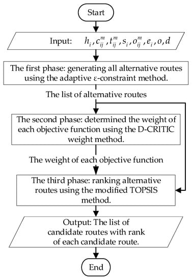
Figure 1.
A flow chart of the proposed approach.
3.1. Generating All Pareto Solutions
This phase involves generating all alternative routes or Pareto solutions using Kirlik and Sayin’s adaptive ε-constraint method []. The adaptive ε-constraint method of Kirlik and Sayın is the ECM with a search mechanism based on the generation of rectangles, as in Laumanns et al. [], and some of the rectangles can be removed if no Pareto solution can be found. The set of feasible outcomes in the objective space is defined as each feasible solution x ∈ X, which is mapped into its corresponding objective vector y = f(x). Since ε is in () dimensional space, the search is managed in .
This method is classified as an exact solution to multi-objective integer optimization problems with more than three objective functions []. This allows for decision makers to obtain the most significant number of alternative routes. This method was selected for the following reasons: (1) This method allows for decision makers to obtain all Pareto solutions or alternative routes. As a result, decision makers have access to as many optimal routes as possible for customers to consider during negotiations of outsourcing transportation operations. (2) Currently, MTOs already use ECM. If they switch to using this method based on the ECM, it will make it easy for planners to understand the principles of solving the problem, because this method is based on the ECM as well. (3) From the computational results in the article by Kirlik and Sayın [], it can be seen that this method is more efficient than previous algorithms in terms of both computational time and the number of models solved per Pareto solution. A flow chart of Kirlik and Sayin’s adaptive ε-constraint method is illustrated in Figure 2.
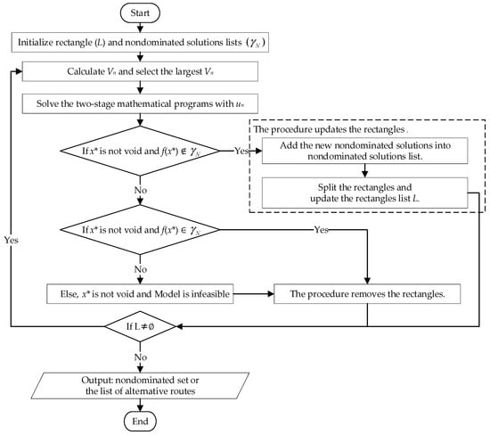
Figure 2.
A flow chart of Kirlik and Sayin’s adaptive ε-constraint method [].
The solution steps of Kirlik and Sayin’s adaptive ε-constraint method [] are as follows.
Step 1: Find the lower bound of a rectangle () by minimizing each single-objective function for p = {2, …, P} as in Equation (11), subject to constraints (7)–(10).
subject to Constraints (7)–(10).
Step 2: Find the upper bound of a rectangle () by maximizing each single-objective function for all p ∈ {2, …, P} as in Equation (12), subject to constraints (7)–(10).
subject to Constraints (7)–(10).
The definitions of and in Equations (5) and (6) can be changed to that in Equations (13) and (14) to ensure that the solution of the upper bound is possible.
The lower bound and upper bound are provided from steps 1 and 2. Then, and are defined in , where and . Therefore, an initial rectangle can be defined as . The lower and upper bounds of the ()-dimensional rectangle are shown in Figure 3.
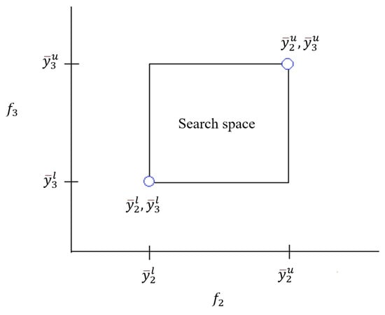
Figure 3.
The projected points of the lower and upper forms of the () dimensional rectangles in the search space.
Step 3: Calculate the volume measure associated with all rectangles for iteration n (Vn), as shown in Equation (15). Then, a rectangle with a larger Vn is selected.
Step 4: The objective function p is kept as the objective function in Kq(ε) (in this paper, the objective function is set as q = 1), while the other values are converted into constraints []. The εp values are on the plane and the projection of all Pareto solutions in . and are defined as the lower and upper vertices of the rectangle, respectively. Therefore, a rectangle is defined as []. The two-stage mathematical programs K1(un) and Q1(un) are solved using the selected rectangle’s upper vertex un as ε. For each rectangle, two-stage optimization problems are solved to avoid weakly efficient solutions, and Kq(ε) and Qq(ε) are defined as follows:
subject to
Constrains (7)–(10).
Consider z* of the sub-problem Kq(ε) in the second stage formulation Qq(ε). Define x* as the optimal solution of two-stage formulations, with x* always efficient for any ε ∈ .
subject to
Constrains (7)–(10).
Step 5: If an optimal solution of two-stage formulations (x*) is not void, and f(x*) is not a member in the Pareto solutions list (), x* is a new Pareto solution and can be added into (). Otherwise, step 8 is followed.
Step 6: is defined as the projection of the new Pareto solution for objective function p. Split the rectangles that satisfy , and then rectangle Rn can be split into two rectangles along the axis. The first resulting rectangle has . The second resulting rectangle has . Then, the list of rectangles L can be updated. The pseudo-code for the procedure updates the rectangles, as shown in Figure 4.
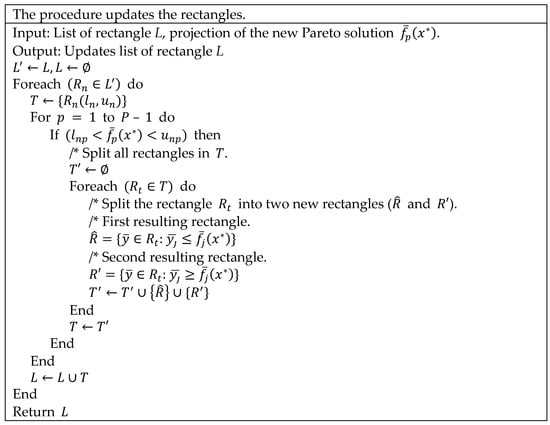
Figure 4.
The procedure updates the rectangles [].
Step 7: The rectangles in which the volume between the upper vertex of the rectangle and do not need to be searched when x* is an optimal solution of two-stage programs P1(un) and Q1(un) are removed. Then, there no Pareto solution is mapped into other than f(x*). The pseudo-code for the procedure removes the rectangles, as shown in Figure 5.
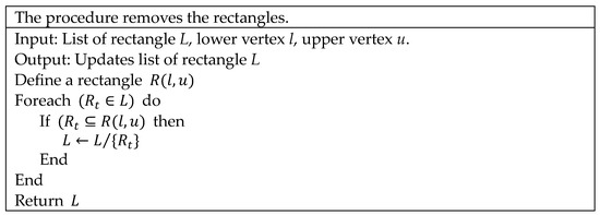
Figure 5.
The procedure removes the rectangles [].
Step 8: If x* is not void, and f(x*) is a member in the Pareto solution list (), remove the rectangle for iteration n using the procedure, which removes the rectangles in step 7. Otherwise, the next step is employed.
Step 9: If x* is void, or the model is infeasible, there is no Pareto solution that is mapped into the rectangle ; all such rectangles will be removed using the procedure that removes the rectangles in step 7.
Step 10: If the list of rectangles is empty (L≠∅), the algorithm is ended and returns all Pareto solutions or all alternative routes. Otherwise, step 3 is followed.
3.2. Determination of the Weight of Each Objective Function
The weight of each objective function can be determined using the D-CRITIC method. The D-CRITIC method [] was developed by incorporating the concept of distance correlation into the traditional CRITIC method [] to improve the shortcomings in denoting the conflicting relationships between the criteria of the Pearson’s correlation [] in the original CRITIC method [,]. The steps of the D-CRITIC method are as follows.
Step 1: Obtain all alternative routes from the first phase to generate the decision matrix, as shown in Table 2. r is defined as the alternative route (r ∈ AR), c is the criterion or objective function (c ∈ C, in this paper C = 3), and is the objective function f(x) of alternative route r with respect to criterion c.
Table 2.
The decision matrix.
Step 2: Normalize the decision matrix, using Equation (21) to transform into standard scales, which range between 0 and 1:
where is the normalized score of alternative route r with respect to criterion c, is the best objective function of criterion c, and is the worst objective function of criterion c.
Step 3: Calculate the standard deviation of criterion c using Equation (22). Define as the mean objective function of criterion c, and AR is the total number of alternatives.
Step 4: Calculate the distance correlation introduced by Székely et al. [] for capturing the conflicting relationships between criteria and criteria using Equation (23) []:
where is the distance covariance between criteria and criteria , is the distance variance of criteria , and is the distance variance of criteria [].
Step 5: Calculate the information content contained in criterion (Ic) using Equation (24):
Step 6: Determined the final objective weight of criterion c using Equation (25). Define Wc as the objective weight of criterion .
3.3. Ranking Alternative Routes
The final phase of the proposed approach is to rank alternative routes using the modified TOPSIS method []. The main justifications for employing the modified TOPSIS method are as follows: (1) The modified TOPSIS method is relatively straightforward to understand and implement. Its simplicity allows for decision makers to easily interpret the results and make informed choices. (2) The method allows for an ability to provide a clear actionable ranking of alternatives based on multiple criteria. (3) The modified TOPSIS method considers both positive (best) and negative (worst) ideal solutions. This makes it more robust and applicable to real-world scenarios. The modified TOPSIS method [] comprises the following steps.
Step 1: Normalize the decision matrix using Equation (26). Define as the normalized performance ratings of alternative route r with respect to criterion c.
Step 2: Calculate the positive ideal solutions () and negative ideal solutions () from the normalized decision matrix.
where
Step 3: Calculate the weighted Euclidean distance using Equations (31) and (32). Define as the positive weighted Euclidean distance, as the negative weighted Euclidean distance, and as the objective weight of criterion c (obtained from Section 3.2).
Step 4: Calculate the overall performance score for each alternative route , as in Equation (33):
Step 5: Rank the competing alternative routes by utilizing the performance score. An alternative route r with higher scores indicates a better alternative performance [,]. Therefore, decision makers can present the alternative route with the highest performance score to the customer for consideration first.
4. Results
In this study, the proposed approach was applied to a real case study to select the best route for transporting bulk cargo (mainly coal) from the anchorage area in the Gulf of Thailand to the destination factory via a multimodal transportation network in Thailand. The multimodal transportation network has 83 nodes and 9579 transportation links, consisting of the load discharge area in the Gulf of Thailand (node 83), the destination factory (node 73), 12 nodes for the seaport, 32 nodes for the river port, 30 nodes for the warehouse, and 4 nodes for the railway station, as shown in Figure 6. There are four modes of transportation: dump trucks, barges, trains, and vessels. Each transport task has a capacity of 20,000 tons, equivalent to a vessel’s capacity. Different types of lines were used to represent the mode of transportation. One mode of transportation could be used for one transportation link. Each transportation link has a different distance. The branch-and-cut algorithm in OpenSolver 2.9.0 was used with the default configuration settings to solve this problem on a computer with an AMD Ryzen 5 4600 H 3.00 GHz and 16 GB RAM. The collected instances and parameters from July to October 2022 are available for download through the following URL: https://sites.google.com/site/transportationlibrary/instance/p11 (accessed on 5 July 2023).
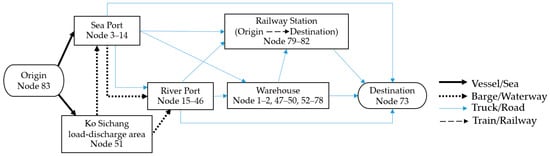
Figure 6.
The multimodal transportation network in Thailand used in this case study.
Multimodal transport operators (MTOs) have to solve multi-objective multimodal routing problems with predetermined origins and destinations traveling through the multimodal transport network in Thailand using the ε-constraint method []. was defined as the number of solutions for objective p to generate the Pareto solution ( = 1, 2, …, ). The decision makers can set the epsilon values ε2 and ε3 to extract the Pareto-optimal solution using Equation (34) [].
In addition, there is no guideline for selecting the appropriate transportation route for customer negotiations. Thus, this current approach relies on decision maker experience in selecting routes from the Pareto solution set for customer negotiations. The MTO needs an approach that provides the most Pareto solutions and an appropriate route selection guideline for negotiating with the customer; there must be various Pareto solutions that decision makers can present to the customer.
4.1. Single-Objective Optimization Results
The first phase of the proposed method was initially solved by considering single objectives of f2(x) and f3(x) separately to determine the lower and upper bounds for assigning the epsilon values (ε2, ε3). The lower and upper bounds of each objective function were obtained from the exact linear solver, as shown in Table 3.
Table 3.
The lower and upper bounds of each objective function.
4.2. Multi-Objective Optimization Results
In this section, the Pareto fronts obtained from the proposed approach (PA) based on the adaptive ε-constraint method of Kirlik and Sayin [] and the current approach based on the ε-constraint method (ECM) [] with differences in the epsilon value settings were compared to assess the effectiveness of the proposed approach in terms of the number of Pareto solutions found (NPS) and the computational time (CPU). The three scenarios were defined in setting the epsilon values ε2 and ε3 in the ECM compared with the PA by changing the values in Equation (34) as follows: situation 1 (ECM 4 × 4) is set as = 4 and = 4, situation 2 (ECM 6 × 6) is set as = 6 and = 6, and situation 3 (ECM 10 × 10) is set as = 10 and = 10. The Pareto solutions obtained and the computational time of the current and the proposed methods are presented in Table 4.
Table 4.
Comparison of the proposed and current approaches with differences in epsilon value settings.
Table 4 demonstrates that the proposed approach can identify Pareto solutions more than ECM 4 × 4, ECM 6 × 6, and ECM 10 × 10 by 133.33%, 75.00%, and 16.67%, respectively. Moreover, the proposed method took the least computational time per Pareto solution compared to ECM 4 × 4, ECM 6 × 6, and ECM 10 × 10, by 15.52%, 51.96%, and 76.74%, respectively. The proposed method was more efficient than the current method for all experiments that changed the epsilon value settings in terms of the number of Pareto solutions found and the ratio of computational time to the number of Pareto solutions found. The Pareto frontier obtained from the proposed method indicates that increasing the total cost (f1) decreases the total time (f2) and the total CO2e emissions (f3), as shown in Figure 7.
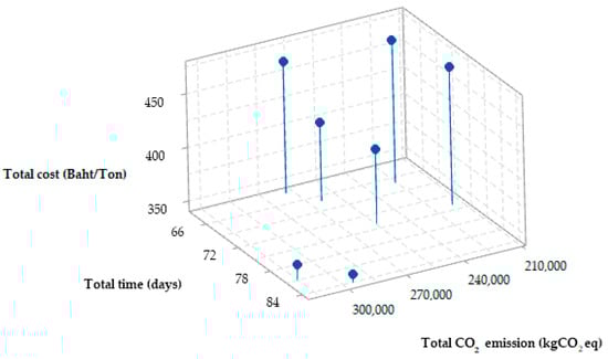
Figure 7.
The Pareto frontier obtained from the proposed method for case study problem.
4.3. Pareto Solution Ranking Results
The results of the Pareto solution ranking were obtained using modified TOPSIS [] with the D-CRITIC weighting method [], identified in this section. The weights of three objective functions using the D-CRITIC method are presented in Table 5.
Table 5.
Weight of three objective functions using the D-CRITIC method.
After calculating the criteria weights, the next step was to apply modified TOPSIS [] to calculate the overall performance score (OPr) matrix. The results of the OPr matrix for Pareto solutions are presented in Table 6.
Table 6.
The overall performance score (OPr) matrix for Pareto solutions of the proposed method.
It is evident from Table 6 that Pareto solution number 7 had the highest overall performance score value, at 0.5929, among all seven solutions, having a total cost of 472.73 baht/tons, a total time of 67 days, and total CO2e emissions of 225,396.08 kgCO2eq. Therefore, Pareto solution no. 7 is the first choice that decision makers can present to their customers. If the customer is not interested in Pareto solution number 7, the decision maker will offer Pareto solution numbers 4, 5, 3, 6, 1, and 2, respectively.
5. Conclusions
This study applied Kirlik and Sayin’s adaptive ε-constraint method [] for generating all Pareto solutions, and then ranked the Pareto solutions using the modified TOPSIS [] with the D-CRITIC weighting method [] to solve the multimodal routing problem (MRP) of bulk transportation in Thailand, with the aim of minimizing the total cost, transportation time, and total carbon dioxide-equivalent (CO2e) emissions simultaneously. For this case study, the decision maker had to choose an appropriate route from the Gulf of Thailand to the destination plant, through the multimodal transportation network in Thailand, for presentation to the customer during the negotiation process for outsourcing transportation.
The computational results indicate that the proposed approach exhibits superior performance to the current approach based on the ε-constraint method in terms of the number of Pareto solutions found and the ratio of computational time to the number of Pareto solutions found. In addition, the proposed approach also provides a rank for deciding the appropriate route for customers, whereas the current method applied to case studies still requires the decision maker’s experience to choose a route to present to the customer.
From a theoretical perspective, this paper contributes the following: First, a novel multi-criteria decision-making approach was introduced for the MTRP with three or more objective functions. Second, this is the first time that the adaptive ε-constraint method of Kirlik and Sayın [] has been applied to find all Pareto solutions for the MRP. This approach could be the basis for starting further work to solve the MRP.
Regarding practical implications, this paper proposes several implications on the practical side of things: First, the proposed approach provides assistance to decision makers in selecting the best route and ranks other alternative routes from different perspectives. Additionally, it increases the likelihood that the MTO will reach an agreement with its customers. Second, the integrated weighting method and MADM allow for practitioners and managers to prioritize alternatives quickly and efficiently without relying on expert experience or decision makers. MTOs can benefit significantly from this proposed approach, especially when decision makers require an accurate ranking of the possible alternative routes.
In the future, a novel approach should be developed for the fuzzy multimodal routing problem with uncertain transportation times due to traffic conditions and other factors to obtain the most suitable transportation routes and acceptable computational times. In addition, objective considerations of social impacts and risks need to be added to the mathematical model to enable more comprehensive decision making.
Funding
This research was funded by College of Industrial Technology, King Mongkut’s University of Technology North Bangkok (Grant No. Res-CIT0272/2021).
Institutional Review Board Statement
Not applicable.
Informed Consent Statement
Not applicable.
Data Availability Statement
The data presented in this study are available on request from the corresponding author or for download at: https://sites.google.com/site/transportationlibrary/instance/p11 (accessed on 1 August 2023).
Acknowledgments
This research was funded by College of Industrial Technology, King Mongkut’s University of Technology North Bangkok (Grant No. Res-CIT0272/2021). The author would like to thank the multimodal transport operator in Central Thailand for providing transportation data and insight.
Conflicts of Interest
The author declares no conflict of interest.
Nomenclatures
| Abbreviation | |
| AECM | Augmented ε-constraint method |
| AHP | Analytic hierarchy process |
| BWM | Best–worst method |
| CILOS | Criterion Impact Loss |
| CO2e | Carbon dioxide-equivalent |
| COE | CO2 emissions |
| CP | Compromise programming technique with different distance metrics |
| CPU | Computational time |
| CPU/NPS | Ratio of computational time to the number of Pareto solutions found |
| CRITIC | CRITIC weight method |
| D-CRITIC | Distance Correlation-based Criteria Importance Through Inter-criteria Correlation |
| DEA | Data envelopment analysis |
| DRSA | Dominance-based rough set approach |
| ECM | ε-constraint method |
| FCC | Fuzzy credibility chance constraint |
| FGP-DIP | Fuzzy goal programming approach with different importance and priorities |
| FUCOM | Full Consistency Method |
| GA | Genetic algorithm |
| GP | Goal programing model |
| GRAS | Greedy randomized adaptive search procedure |
| IDOCRIW | Integrated Determination of Objective CRIteria Weights |
| IFGP | Interactive fuzzy goal programming approach |
| ILS | Iterated local search |
| LBWA | Level Based Weight Assessment |
| LT | Linearization technique |
| MACA | Multi-objective ant colony algorithm |
| MADM | Multiple-attribute decision-making method |
| MEREC | MEthod based on the Removal Effects of Criteria |
| MODM | Multiple-objective decision-making method |
| MOGA | Multi-objective genetic algorithm |
| MOTGA | Multi-objective Taguchi genetic algorithm |
| MRP | Multimodal routing problem |
| MTO | Multimodal transport operator |
| NNCM | Normalized normal constraint method |
| NPS | The number of Pareto solutions found |
| NSGA | Non-dominated sorting genetic algorithm |
| PA | Proposed approach |
| SAPEVO-M | Simple Aggregation of Preferences Expressed by Ordinal Vectors Group Decision Making |
| SWARA | Step-wise weight assessment ratio analysis method |
| TGO | Thailand Greenhouse Gas Management Organization |
| TOPSIS | Technique for order of preference by similarity to ideal solution |
| TOPSIS | Technique for order of preference by similarity to ideal solution modified method |
| TSM | Tabu search methodology |
| VIKOR | Vlse Kriterijumska Optimizacija I Kompromisno Resenje |
| WFGP | Weighted additive fuzzy goal programming approach |
| WMN | Weighting sum method with normalization |
| WSM | Weighting sum method |
| ZOGP | Zero-one goal programming |
| Sets and Subscript | |
| c | The criterion or objective function (c ∈ C, in this paper C = 3) |
| E | The set of transportation links (i, j) ∈ E |
| The set of solutions for objective p to generate the Pareto solution ( = 1, 2, …, ) | |
| l | Lower bounds |
| M | The set of transportation modes m ∈ M |
| n | Iteration for search algorithm in adaptive ε-constraint method |
| P | The set of objective functions p ∈ P |
| q | The first objective functions (q = 1, q≠ p) |
| r | The alternative route (r ∈ AR) |
| u | Upper bounds |
| V | The set of nodes (terminals) i ∈ V, j ∈ V |
| X | The set of feasible solutions x ∈ X |
| Parameters and variables | |
| The mean objective function of criterion c | |
| The best objective function of criterion c | |
| The worst objective function of criterion c | |
| The objective function f(x) of alternative route r with respect to criterion c | |
| The normalized score of alternative route r with respect to criterion c | |
| Alternative route with the highest normalized performance score in terms of criterion c | |
| Alternative route with the minimum normalized performance score in terms of criterion c | |
| The normalized performance ratings of alternative route r with respect to criterion c | |
| Transportation cost from terminals i to j by transportation mode m (Baht/ton) | |
| d | Destination terminal |
| The conflicting relationships between criteria c and criteria c’ | |
| The distance covariance between criteria c and criteria c’ | |
| CO2e emissions at terminal i (kgCO2e) | |
| fp(x) | The objective function value of objective function p |
| fq(x) | The objective function value of objective function q |
| f(x*) | The objective function value of new Pareto solution |
| Projection of new Pareto solution for objective function p | |
| Transshipment cost at terminal i (Baht/ton) | |
| Ic | The information content contained in criterion c |
| Kq(un) | The objective function in first stage of the two-stage mathematical programs |
| L | List of rectangles |
| ln | Lower bounds of iteration n |
| CO2e emissions from terminals i to j by transportation mode m when i ≠ j (kgCO2e) | |
| CO2e emissions from terminals i to j by transportation mode m (kgCO2e) | |
| The overall performance score for each alternative route | |
| Qp(un) | The objective function in the second stage of the two-stage mathematical programs |
| Rn | Rectangle of iteration n |
| Service time at terminal i (hours) | |
| The standard deviation of criterion c | |
| Transportation time from terminals i to j by transportation mode m when i ≠ j (hours) | |
| Transportation time from terminals i to j by transportation mode m (hours) | |
| un | Upper bounds of iteration n |
| The upper bound of objective functions p for iteration n | |
| The volume measure associated with all rectangles for iteration n | |
| The objective weight of criterion c | |
| The positive weighted Euclidean distance | |
| The negative weighted Euclidean distance | |
| Binary decision variables: 1 = if the goods are transported from terminals i to j by transportation mode m and transshipped at terminal i; 0 = otherwise | |
| x* | The optimal solution of two-stage formulations Kq(un) and Qq(un) |
| y | Corresponding objective vector |
| Projection of corresponding objective vector | |
| The lower vertex of a rectangle for dimension p | |
| The upper vertex of a rectangle for dimension p | |
| The optimal objective value of subproblem Kq(un). | |
| 0 | Origin terminal |
| Positive ideal solutions | |
| Negative ideal solutions | |
| ε | ε-constraint value |
| Large number (σ = 999,999) | |
| The Pareto solutions list | |
References
- UNECE. Glossary for Transport Statistics, 5th ed.; Publications Office of the European Unio: Luxembourg, 2019; ISBN 978-92-76-06213-4. [Google Scholar]
- Crainic, T. International Series in Operations Research & Management Science. In Handbook of Transportation Science; Hall, R., Ed.; Springer U.S.: New York, NY, USA, 2003; pp. 451–516. ISBN 978-0-306-48058-4. [Google Scholar]
- Elbert, R.; Müller, J.P.; Rentschler, J. Tactical network planning and design in multimodal transportation—A systematic literature review. Res. Transp. Bus. Manag. 2020, 35, 100462. [Google Scholar] [CrossRef]
- Laurent, A.B.; Vallerand, S.; van der Meer, Y.; D’Amours, S. CarbonRoadMap: A multicriteria decision tool for multimodal transportation. Int. J. Sustain. Transp. 2020, 14, 205–214. [Google Scholar] [CrossRef]
- Yang, X.; Low, J.M.W.; Tang, L.C. Analysis of intermodal freight from China to Indian Ocean: A goal programming approach. J. Transp. Geogr. 2011, 19, 515–527. [Google Scholar] [CrossRef]
- Verma, M.; Verter, V.; Zufferey, N. A bi-objective model for planning and managing rail-truck intermodal transportation of hazardous materials. Transp. Res. Part E Logist. Transp. Rev. 2012, 48, 132–149. [Google Scholar] [CrossRef]
- Kengpol, A.; Meethom, W.; Tuominen, M. The development of a decision support system in multimodal transportation routing within Greater Mekong sub-region countries. Int. J. Prod. Econ. 2012, 140, 691–701. [Google Scholar] [CrossRef]
- Demir, E.; Hrušovský, M.; Jammernegg, W.; Van Woensel, T.; Demir, E.; Hrušovský, M.; Jammernegg, W.; Van Woensel, T.; Sun, Y.; Lang, M.; et al. Best routes selection in multimodal networks using multi-objective genetic algorithm. Sustain. Artic. 2018, 9, 655–673. [Google Scholar]
- Kengpol, A.; Tuammee, S.; Tuominen, M. The development of a framework for route selection in multimodal transportation. Int. J. Logist. Manag. 2014, 25, 581–610. [Google Scholar] [CrossRef]
- Sun, Y.; Lang, M. Bi-objective optimization for multi-modal transportation routing planning problem based on pareto optimality. J. Ind. Eng. Manag. 2015, 8, 1195–1217. [Google Scholar] [CrossRef]
- Assadipour, G.; Ke, G.Y.; Verma, M. Planning and managing intermodal transportation of hazardous materials with capacity selection and congestion. Transp. Res. Part E Logist. Transp. Rev. 2015, 76, 45–57. [Google Scholar] [CrossRef]
- Resat, H.G.; Turkay, M. Design and operation of intermodal transportation network in the Marmara region of Turkey. Transp. Res. Part E Logist. Transp. Rev. 2015, 83, 16–33. [Google Scholar] [CrossRef]
- Baykasoğlu, A.; Subulan, K. A multi-objective sustainable load planning model for intermodal transportation networks with a real-life application. Transp. Res. Part E Logist. Transp. Rev. 2016, 95, 207–247. [Google Scholar] [CrossRef]
- Sun, Y.; Lang, M.; Wang, D. Bi-objective modelling for hazardous materials road–rail multimodal routing problem with railway schedule-based space–time constraints. Int. J. Environ. Res. Public Health 2016, 13, 762. [Google Scholar] [CrossRef] [PubMed]
- Abbassi, A.; Elhilali, A.; Boukachour, J. Modelling and solving a bi-objective intermodal transport problem of agricultural products. Int. J. Ind. Eng. Comput. 2018, 9, 439–460. [Google Scholar] [CrossRef]
- Sun, Y.; Li, X.; Liang, X.; Zhang, C. A bi-objective fuzzy credibilistic chance-constrained programming approach for the hazardous materials road-rail multimodal routing problem under uncertainty and sustainability. Sustainability 2019, 11, 2577. [Google Scholar] [CrossRef]
- Demir, E.; Hrušovský, M.; Jammernegg, W.; Van Woensel, T.; Demir, E.; Hrušovský, M.; Jammernegg, W.; Van Woensel, T. Green intermodal freight transportation: Bi-objective modelling and analysis. Int. J. Prod. Res. 2019, 57, 6162–6180. [Google Scholar] [CrossRef]
- Chen, D.; Zhang, Y.; Gao, L.; Thompson, R.G. Optimizing Multimodal Transportation Routes Considering Container Use. Sustain. Artic. 2019, 11, 5320. [Google Scholar] [CrossRef]
- Sun, Y. A Fuzzy Multi-Objective Routing Model for Managing Hazardous Materials Door-to-Door Transportation in the Road-Rail Multimodal Network with Uncertain Demand and Improved Service Level. IEEE Access 2020, 8, 172808–172828. [Google Scholar] [CrossRef]
- Liaqait, R.A.; Warsi, S.S.; Agha, M.H.; Zahid, T.; Becker, T. A multi-criteria decision framework for sustainable supplier selection and order allocation using multi-objective optimization and fuzzy approach. Eng. Optim. 2022, 54, 928–948. [Google Scholar] [CrossRef]
- Koohathongsumrit, N.; Meethom, W. An integrated approach of fuzzy risk assessment model and data envelopment analysis for route selection in multimodal transportation networks. Expert Syst. Appl. 2021, 171, 114342. [Google Scholar] [CrossRef]
- Zhu, C.; Zhu, X. Multi-Objective Path-Decision Model of Multimodal Transport Considering Uncertain Conditions and Carbon Emission Policies. Symmetry 2022, 14, 221. [Google Scholar] [CrossRef]
- Koohathongsumrit, N.; Meethom, W. Route selection in multimodal transportation networks: A hybrid multiple criteria decision-making approach. J. Ind. Prod. Eng. 2021, 38, 171–185. [Google Scholar] [CrossRef]
- Zhang, H.; Li, Y.; Zhang, Q.; Chen, D. Route Selection of Multimodal Transport Based on China Railway Transportation. J. Adv. Transp. 2021, 2021, 9984659. [Google Scholar] [CrossRef]
- Koohathongsumrit, N.; Chankham, W. A hybrid approach of fuzzy risk assessment-based incenter of centroid and MCDM methods for multimodal transportation route selection. Cogent Eng. 2022, 9, 110167. [Google Scholar] [CrossRef]
- Shao, C.; Wang, H.; Yu, M. Multi-Objective Optimization of Customer-Centered Intermodal Freight Routing Problem Based on the Combination of DRSA and NSGA-III. Sustainability 2022, 14, 2985. [Google Scholar] [CrossRef]
- Baykasoğlu, A.; Subulan, K.; Taşan, A.S.; Dudaklı, N. A review of fleet planning problems in single and multimodal transportation systems. Transp. A Transp. Sci. 2019, 15, 631–697. [Google Scholar] [CrossRef]
- Mesquita-Cunha, M.; Figueira, J.R.; Barbosa-Póvoa, A.P. New–constraint methods for multi-objective integer linear programming: A Pareto front representation approach. Eur. J. Oper. Res. 2023, 306, 286–307. [Google Scholar] [CrossRef]
- SteadieSeifi, M.; Dellaert, N.P.; Nuijten, W.; Van Woensel, T.; Raoufi, R. Multimodal freight transportation planning: A literature review. Eur. J. Oper. Res. 2014, 233, 1–15. [Google Scholar] [CrossRef]
- Deluka-Tibljaš, A.; Karleuša, B.; Dragičević, N.; Aleksandra Deluka-Tibljaš, Ü. Review of multicriteria-analysis methods application in decision making about transport infrastructure. Građevinar 2013, 65, 619–631. [Google Scholar] [CrossRef]
- Yannis, G.; Kopsacheili, A.; Dragomanovits, A.; Petraki, V. State-of-the-art review on multi-criteria decision-making in the transport sector. J. Traffic Transp. Eng. 2020, 7, 413–431. [Google Scholar] [CrossRef]
- Tirkolaee, E.B.; Abbasian, P.; Weber, G.-W. Sustainable fuzzy multi-trip location-routing problem for medical waste management during the COVID-19 outbreak. Sci. Total Environ. 2021, 756, 143607. [Google Scholar] [CrossRef]
- Lo, H.W.; Liaw, C.F.; Gul, M.; Lin, K.Y. Sustainable supplier evaluation and transportation planning in multi-level supply chain networks using multi-attribute- and multi-objective decision making. Comput. Ind. Eng. 2021, 162, 107756. [Google Scholar] [CrossRef]
- Aktar, M.S.; De, M.; Mazumder, S.K.; Maiti, M. Multi-objective green 4-dimensional transportation problems for damageable items through type-2 fuzzy random goal programming. Appl. Soft Comput. 2022, 130, 109681. [Google Scholar] [CrossRef]
- Chhibber, D.; Srivastava, P.K.; Bisht, D.C.S. Intuitionistic fuzzy TOPSIS for non-linear multi-objective transportation and manufacturing problem. Expert Syst. Appl. 2022, 210, 118357. [Google Scholar] [CrossRef]
- Goli, A.; Babaee Tirkolaee, E.; Golmohammadi, A.-M.; Atan, Z.; Weber, G.-W.; Ali, S.S. A robust optimization model to design an IoT-based sustainable supply chain network with flexibility. Cent. Eur. J. Oper. Res. 2023. [Google Scholar] [CrossRef]
- Babaei, A.; Khedmati, M.; Jokar, M.R.A.; Tirkolaee, E.B. An integrated decision support system to achieve sustainable development in transportation routes with traffic flow. Environ. Sci. Pollut. Res. 2023, 30, 60367–60382. [Google Scholar] [CrossRef]
- Tirkolaee, E.B.; Goli, A.; Mardani, A. A novel two-echelon hierarchical location-allocation-routing optimization for green energy-efficient logistics systems. Ann. Oper. Res. 2023, 324, 795–823. [Google Scholar] [CrossRef]
- Simić, V.; Milovanović, B.; Pantelić, S.; Pamučar, D.; Tirkolaee, E.B. Sustainable route selection of petroleum transportation using a type-2 neutrosophic number based ITARA-EDAS model. Inf. Sci. 2023, 622, 732–754. [Google Scholar] [CrossRef]
- Tirkolaee, E.B.; Goli, A.; Gütmen, S.; Weber, G.-W.; Szwedzka, K. A novel model for sustainable waste collection arc routing problem: Pareto-based algorithms. Ann. Oper. Res. 2023, 324, 189–214. [Google Scholar] [CrossRef] [PubMed]
- Wang, Y.; Roy, N.; Zhang, B. Multi-objective transportation route optimization for hazardous materials based on GIS. J. Loss Prev. Process Ind. 2023, 81, 104954. [Google Scholar] [CrossRef]
- Oudani, M. A combined multi-objective multi criteria approach for blockchain-based synchromodal transportation. Comput. Ind. Eng. 2023, 176, 108996. [Google Scholar] [CrossRef]
- Ayan, B.; Abacıoğlu, S.; Basilio, M.P. A Comprehensive Review of the Novel Weighting Methods for Multi-Criteria Decision-Making. Information 2023, 14, 285. [Google Scholar] [CrossRef]
- Krishnan, A.R.; Kasim, M.M.; Hamid, R.; Ghazali, M.F. A Modified CRITIC Method to Estimate the Objective Weights of Decision Criteria. Symmetry 2021, 13, 973. [Google Scholar] [CrossRef]
- Odu, G.O. Weighting methods for multi-criteria decision making technique. J. Appl. Sci. Environ. Manag. 2019, 23, 1449. [Google Scholar] [CrossRef]
- Ma, J.; Fan, Z.-P.; Huang, L.-H. A subjective and objective integrated approach to determine attribute weights. Eur. J. Oper. Res. 1999, 112, 397–404. [Google Scholar] [CrossRef]
- Mahmoody Vanolya, N.; Jelokhani-Niaraki, M. The use of subjective–objective weights in GIS-based multi-criteria decision analysis for flood hazard assessment: A case study in Mazandaran, Iran. GeoJournal 2021, 86, 379–398. [Google Scholar] [CrossRef]
- Krishnan, A.R.; Mat Kasim, M.; Hamid, R. An Alternate Unsupervised Technique Based on Distance Correlation and Shannon Entropy to Estimate λ0-Fuzzy Measure. Symmetry 2020, 12, 1708. [Google Scholar] [CrossRef]
- Jahan, A.; Mustapha, F.; Sapuan, S.M.; Ismail, M.Y.; Bahraminasab, M. A framework for weighting of criteria in ranking stage of material selection process. Int. J. Adv. Manuf. Technol. 2012, 58, 411–420. [Google Scholar] [CrossRef]
- Singh, M.; Pant, M. A review of selected weighing methods in MCDM with a case study. Int. J. Syst. Assur. Eng. Manag. 2021, 12, 126–144. [Google Scholar] [CrossRef]
- Rezaei, J. Best-worst multi-criteria decision-making method. Omega 2015, 53, 49–57. [Google Scholar] [CrossRef]
- Zavadskas, E.K.; Podvezko, V. Integrated Determination of Objective Criteria Weights in MCDM. Int. J. Inf. Technol. Decis. Mak. 2016, 15, 267–283. [Google Scholar] [CrossRef]
- Pamučar, D.; Stević, Ž.; Sremac, S. A New Model for Determining Weight Coefficients of Criteria in MCDM Models: Full Consistency Method (FUCOM). Symmetry 2018, 10, 393. [Google Scholar] [CrossRef]
- Žižović, M.; Pamučar, D. New model for determining criteria weights: Level Based Weight Assessment (LBWA) model. Decis. Mak. Appl. Manag. Eng. 2019, 2, 126–137. [Google Scholar] [CrossRef]
- Gomes, C.F.S.; dos Santos, M.; Teixeira, L.F.H.d.S.d.B.; Sanseverino, A.M.; Barcelos, M.R.d.S. SAPEVO-M: A Group Multicriteria Ordinal Ranking Method. Pesqui. Oper. 2020, 40, e226524. [Google Scholar] [CrossRef]
- Keshavarz-Ghorabaee, M.; Amiri, M.; Zavadskas, E.K.; Turskis, Z.; Antucheviciene, J. Determination of Objective Weights Using a New Method Based on the Removal Effects of Criteria (MEREC). Symmetry 2021, 13, 525. [Google Scholar] [CrossRef]
- Kirlik, G.; Sayın, S. A new algorithm for generating all nondominated solutions of multiobjective discrete optimization problems. Eur. J. Oper. Res. 2014, 232, 479–488. [Google Scholar] [CrossRef]
- Maneengam, A. A Bi-Objective Programming Model for Multimodal Transportation Routing Problem of Bulk Cargo Transportation. In Proceedings of the 2020 IEEE 7th International Conference on Industrial Engineering and Applications (ICIEA), Bangkok, Thailand, 16–21 April 2020; IEEE: Bangkok, Thailand, 2020; pp. 890–894. [Google Scholar]
- Thailand Greenhouse Gas Management Organization. Carbon Footprint of Product Guideline, 4th ed.; Thailand Greenhouse Gas Management Organization: Bangkok, Thailand, 2012; ISBN 978-974-286-819-2. [Google Scholar]
- TGO (Thailand Greenhouse Gas Management Organization). Update Emission Factor CFP. Available online: http://thaicarbonlabel.tgo.or.th/admin/uploadfiles/emission/ts_822ebb1ed5.pdf (accessed on 15 January 2019).
- Deng, H.; Yeh, C.-H.; Willis, R.J. Inter-company comparison using modified TOPSIS with objective weights. Comput. Oper. Res. 2000, 27, 963–973. [Google Scholar] [CrossRef]
- Laumanns, M.; Thiele, L.; Zitzler, E. An efficient, adaptive parameter variation scheme for metaheuristics based on the epsilon-constraint method. Eur. J. Oper. Res. 2006, 169, 932–942. [Google Scholar] [CrossRef]
- Bashir, B.; Karsu, Ö. Solution approaches for equitable multiobjective integer programming problems. Ann. Oper. Res. 2022, 311, 967–995. [Google Scholar] [CrossRef]
- Chankong, V.; Haimes, Y.Y. Multiobjective Decision Making: Theory and Methodology; North-Holland/Elsevier Science Publishing Company, Inc.: New York, NY, USA, 1983; ISBN 0444007105. [Google Scholar]
- Horst, R.; Tuy, H. Global Optimization: Deterministic Approaches; Springer Science & Business Media: New York, NY, USA, 2013. [Google Scholar]
- Diakoulaki, D.; Mavrotas, G.; Papayannakis, L. Determining objective weights in multiple criteria problems: The critic method. Comput. Oper. Res. 1995, 22, 763–770. [Google Scholar] [CrossRef]
- Pearson, K. Note on Regression and Inheritance in the Case of Two Parents. Proc. R. Soc. Lond. 1895, 58, 240–242. [Google Scholar]
- Székely, G.J.; Rizzo, M.L.; Bakirov, N.K. Measuring and testing dependence by correlation of distances. Ann. Stat. 2007, 35, 2769–2794. [Google Scholar] [CrossRef]
- Shen, C.; Priebe, C.E.; Vogelstein, J.T. From Distance Correlation to Multiscale Graph Correlation. J. Am. Stat. Assoc. 2020, 115, 280–291. [Google Scholar] [CrossRef]
- Chakraborty, S. TOPSIS and Modified TOPSIS: A comparative analysis. Decis. Anal. J. 2022, 2, 100021. [Google Scholar] [CrossRef]
Disclaimer/Publisher’s Note: The statements, opinions and data contained in all publications are solely those of the individual author(s) and contributor(s) and not of MDPI and/or the editor(s). MDPI and/or the editor(s) disclaim responsibility for any injury to people or property resulting from any ideas, methods, instructions or products referred to in the content. |
© 2023 by the author. Licensee MDPI, Basel, Switzerland. This article is an open access article distributed under the terms and conditions of the Creative Commons Attribution (CC BY) license (https://creativecommons.org/licenses/by/4.0/).