Irrigation Scheduling for Small-Scale Crops Based on Crop Water Content Patterns Derived from UAV Multispectral Imagery

Abstract

A timely irrigation schedule for small-scale farms is imperative for ensuring optimum crop production in the wake of drought and climate change. Owing to the large number of irrigated small-scale farms that grow different crops across all seasons in the Mutale River catchment, this study sought to develop irrigation scheduling for these crops for sustainable water utilization without compromising crop yields. Unmanned aerial vehicle (UAV) images were utilized as the base from which crop water content patterns were derived. A total of four (4) spectral vegetation indices, viz, the Greenness Normalized Difference Vegetation Index (GNDVI), Normalized Difference Vegetation Index (NDVI), Normalized Difference Red-Edge Index (NDRE), and Optimized Soil-Adjusted Vegetation Index (OSAVI), were generated to characterize crop types and water content in this study. Crop water content data, in the form of the relative water content (RWC), were measured in the field for each type of crop. Crop water content was modelled based on the empirical relationships between spectral indices and field-measured RWC. The linear regression analysis revealed a significant association between the GNDVI and the water content of sweet potato, maize, sugar beans, and Florida broadleaf mustard, with r² values of 0.948, 0.995, 0.978, and 0.953, respectively. The NDVI revealed a strong association with the water content of Solanum retroflexum, pepper, and cabbage, with r² values of 0.949, 0.956, and 0.995, respectively. The NDRE, on the other hand, revealed a strong relationship with water content in peas and green beans, with r² values of 0.961 and 0.974, respectively. The crop water content patterns simulation revealed that Solanum retroflexum, sweet potato, maize, sugar beans, and Florida broadleaf mustard reached their respective wilting points on day four after irrigation, implying that irrigation of these crops should be scheduled after every four (4) days. Peas, green beans, pepper, and cabbage reached their respective wilting points on day five after irrigation, implying that irrigation of these crops should be scheduled after every five days. The results of this study highlight the significance of considering crop water content derived from spectral bands of UAV imagery in scheduling irrigation for various types of crops. This study also emphasized the on-going significance of remote sensing technology in addressing agricultural issues that impede hunger alleviation and food security goals.

1. Introduction

Small-scale farms account for over 80% of global agricultural produce [1], despite occupying only 12% of the total global farmlands [2]. These farms are characterized by a low asset base and land plot below 2 hectares [3], where farmers operate under structural constraints such as lack of access to optimum farming resources [4]. Small-scale agricultural practice is often characterized by subsistence crops, with their production almost entirely dependent on family labour [5]. Optimum crop yield in these farms is deemed the key to the provision of practical and sustainable solutions to global hunger, poverty, and local economic challenges [6]. However, low crop yields in these farms are highly attributed to water scarcity [7]. Globally, water input to crop farming has been on the rise [8], responding to the rising food demand posed by the ever-growing population. However, due to unpredictable rainfall in many regions of the world, small-scale crop farming generally relies on irrigation to ensure continuous availability of food [9] As such, timely irrigation scheduling for these farms is imperative for ensuring optimum crop production in the wake of drought and climate change [10]. Irrigated small-scale crops account for at least 40% of the total global food produced [11]. In South Africa, the unreliability of rainfall has underscored the need to shift small-scale farming practice from rainfed to irrigation-based [12]. In the Mutale River catchment of this country, small-scale crop growth and yields are sustained by the irrigation system, especially during the dry season when rainfall is scarce. Various types of crops, such as cabbage, sweet potato, maize, garlic, Florida broadleaf mustard, Solanum retroflexum, green beans, sugar beans, and spinach, are cultivated across all seasons, due to availability of water through the irrigation system. However, the irrigation system in place is based on the “one-size-fits-all” concept, i.e., all types of crops are subjected to the same irrigation scheduling programme, notwithstanding their differences in water requirements. These crops are only irrigated after every seven (7) days as per the devised irrigation scheduling programme. Subsequently, some crop types tend to be irrigated before they reach their respective wilting points, while other crop types undergo severe water stress while awaiting the next irrigation period. When properly implemented, irrigation improves crop yields and subsequently abundant harvest when compared to rain-fed agriculture [13].

Irrigation scheduling mostly relies on the assessment of the amount of water in the soil. Therefore, it must be carried out when the soil water amount drops below a minimum threshold [14,15]. When carried out using conventional methods, soil moisture acquisition is time-consuming, labour-intensive, and sparsely distributed [16]. From a remote sensing perspective, soil moisture content data are obtained by analysing soil spectral reflectance in the shortwave infrared (SWIR) [17,18], thermal infrared (TIR) [19,20,21], and microwave channels of spectrum [22]. However, the deployment of TIR sensors in soil water content retrieval has been hampered by costs associated with sensor acquisition [23]. Optical sensors, such as Sentinel [24], Aster [25], and Landsat [19], have demonstrated their ability to detect soil moisture content using their SWIR and TIR spectral channels. However, their respective spatial resolutions make them unviable for small-scale farm plots less than 10 m in width, such as those in the study area. Moreover, the accuracy of soil moisture content retrieved by these sensors in areas of full crop cover remains questionable. The multispectral unmanned aerial vehicle (UAV) systems, in particular, have recently emerged as a valuable source of high-spatial-resolution remote sensing data, offering substantial benefits in relation to cost and adaptability and a high spatial resolution of few centimetres. However, the lack of the spectral channels relevant for soil moisture content detection makes these sensors unsuitable for monitoring soil moisture. However, UAVs have proven to be capable of providing crop health information based on chlorophyll concentration [26].

The relationship between soil moisture content, crop water content, and subsequently crop health has been extensively acknowledged [14,27,28]. For crop water content to remain sufficient, soil moisture content must also stay adequate [29]. Information on crop water content may aid in the determination of the suitable time to irrigate crops, even before they begin to exhibit symptoms of water stress such leaf withering, slowed growth, and decreased leaf area [30,31,32,33]. In the presence of adequate soil moisture content, crops advance their photosynthetic capacity by increasing the distribution proportion of above-ground biomass [34]. As such, insufficient soil moisture has been noted to substantially correlate with non-photochemical quenching and steady-state fluorescence in light-adapted leaves of crops [35]. The inability of crops to regulate sufficient water in their leaves leads to stomatal closure, subsequently limiting the photosynthetic potential of crops [36,37,38]. Therefore, crop water deficit can be assessed through the analysis of crop foliar chlorophyll concentration [39]. From a multispectral remote sensing perspective, spectral reflectance in the visible and near-infrared regions differs between crops under water stress and healthy crops [26]. Healthy crops tend to strongly absorb at visible wavelengths and reflect more energy at near-infrared wavelengths to enhance photosynthesis [40]. The typical reflectance of crops in the visible-infrared spectrum always increases as crop water content declines [41,42,43,44].

Various studies have employed UAV remote sensing in monitoring crop water content in various regions [45,46,47,48]. However, these studies only monitored the water content of a single crop. This underscores the need to monitor water content in areas with multiple crop types. Owing to the large number of irrigated small-scale farms that cultivate different types of crops across all seasons in the Mutale River catchment, this study was aimed at developing irrigation scheduling for these crops to attain sustainable water utilization without compromising crop yields.

2. Materials and Methods

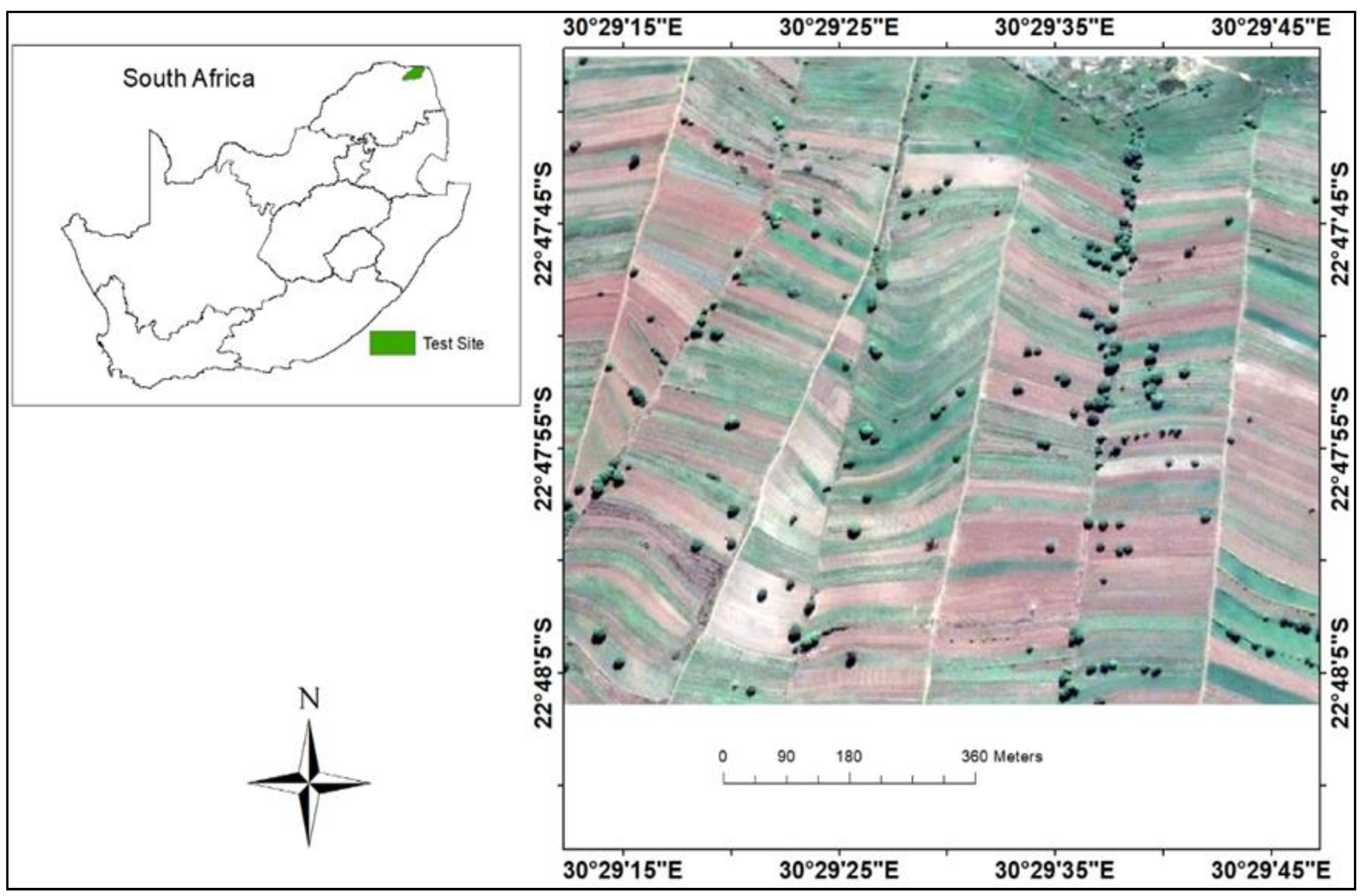
2.1. Study Area

The Mutale River catchment is situated in the Vhembe District, within the Limpopo Province of South Africa. The geographical coordinates of the area are 22°47′50″ S, 30°27′01″ E, and 22°48′13″ S, 30°28′54″ E. The majority of rainfall in this area occurs during the summer months (October to March), while the other three seasons are typically arid [49,50]. The area was selected on the basis of the presence of different types of small-scale crops irrigated under the same schedule. Farmers in the study area practice crop diversification and crop rotation with a variety of crops. The Tshiombo Irrigation Scheme (used for sampling in this study) is the one responsible for supplying water in these small-scale farms [51]. This irrigation scheme obtains water from the Mutale River, which is redirected into a canal, which then channels the water into furrows that are gravity-oriented [52]. The study area is also dominated by the ferrallitic soil type, which is characteristically red in colour, clay-deep, and well-drained with a pH that ranges between 6.0 and 7.0 [53]. Figure 1 shows the locational settings of the study area.

2.2. Data Acquisition

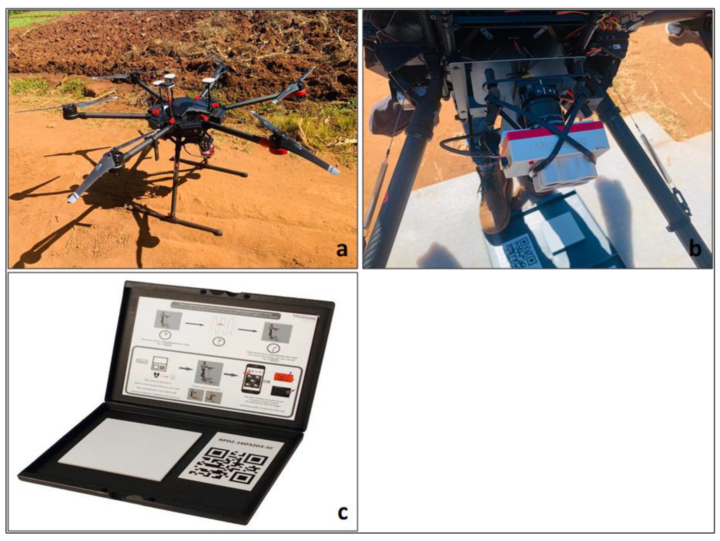
2.2.1. The UAV Data

The UAV imagery used in this study was acquired using the Micasense RedEdge multispectral camera mounted on the DJI Matrice 600 (M600) UAV system provided by the Agricultural Research Council (ARC) of South Africa. The camera was composed of five 3.6 MP, 12-bit sensors with discrete and narrowband filters, capturing images with a spectral range of 475 nm to 840 nm, across 5 bands, i.e., blue (475 nm), green (560 nm), red (668 nm), red edge (717 nm), and NIR (840 nm). The focal length of the camera was 5.5 mm (fixed lens), with a horizontal field of view (HFOV) of 47.2°. Moreover, the camera was equipped with a GPS that finds a location based on signals spanning 24 h. The image resolution of the camera was 1280 mm × 960 mm with a ground sample distance (GSD) of 8.5 cm. The images acquired by this sensor were used in the determination and simulation of crop water content patterns for irrigation scheduling. The UAV system used for crop image acquisition is shown in Figure 2.

2.2.2. Reference Data

Leaf water content data, which are critical for determining crop water stress, were collected in the field from 29 June 2021 to 1 July 2021. The field points marking the locations at which measurements were taken were also recorded using the Garmin eTrex 22x Handheld GPS^®, manufactured by the Garmin Southern Africa (PTY) Ltd., Johannesburg, South Africa. Stratified random sampling was used to collect a total of 9 leaf sample points from each crop type in the study area per day. Thus, a total of 81 sample points were collected for this study per day. The strata for this study were farm plots of the same crop type. Fully developed, no longer growing, and totally illuminated leaves served as the base on which samples were randomly collected from cabbage, Florida broadleaf mustard, sweet potato, peas, green beans, sugar beans, Solanum retroflexum, maize, and pepper. The data included measurements of fresh weight, turgid weight, and dry weight from the sampled crop leaves. A 0.001 g high-precision digital scale was used to record leaf weight. The leaf samples were cut from crops and immediately weighed to obtain their fresh weight (FW), put in resealable plastic bags, and placed in a cooler box with ice cubes for preservation. The leaves were transferred to paper cups and submerged in water for 24 h to obtain the turgid weight (TW). Subsequently, the leaves were air dried for 48 h to obtain the dry weight (DW). Ultimately, crop water content was determined by means of relative water content (RWC) using equation (1) adopted from Gonzalez and Gonzalez-Vilar [54]:

$$\mathrm{R}\mathrm{W}\mathrm{C}=\left[\frac{\mathrm{F}\mathrm{W}-\mathrm{D}\mathrm{W}}{\mathrm{T}\mathrm{W}-\mathrm{D}\mathrm{W}}\right]\times 100$$

(1)

where

FW is the sample’s fresh weight;

TW is the turgid weight;

DW is the dry weight.

Sampling was performed at midday since this is the most stable time of day with respect to irradiance and temperature and their effect on leaf water relations [55]. From a total of nine (9) sample points collected per crop type, five (5) sample points were used for establishing the relationship between the spectral vegetation index and crop water content (i.e., calibration datasets), and the remaining four (4) sample points were used to evaluate the accuracy of the empirical model (validation datasets). This was carried out for all three days on which the UAV imagery was acquired.

2.3. UAV Camera Calibration

Calibration of the sensor before each flight was performed using the Micasense Calibrated Reflectance Panel (CRP). Calibration was performed to realign the sensor with land feature irradiance properties during the flight period. The spectral data in the CRP were provided as the absolute reflectance in the range of 400 nm to 850 nm. Calibration was carried out by taking an image of the CRP before each flight. In an open area with the panel lying flat on the ground, the sensor was held approximately 1 m away while ensuring that the quick response (QR) code was centred in the field of view. The sensor was held facing the direction of the incident light to prevent interference by light reflectance from surrounding objects. Once the sensor detected the panel, it flashed a light-emitting diode indicating a successful capture of incident radiation. The transfer function of radiance to reflectance for each spectral channel was then computed using Equation (2) according to Dang et al. [56]:

$${\mathrm{F}}_{\mathrm{i}}=\frac{{\mathsf{\rho }}_{\mathrm{i}}}{\mathrm{a}\mathrm{v}\mathrm{g}\left({\mathrm{L}}_{\mathrm{i}}\right)}$$

(2)

where

F_i is the reflectance calibration factor for the i^th band;

ρ_i is the average reflectance of the CRP for the i^th band;

avg(L_i) is the average value of the radiance for the pixels inside the panel for the i^th band.

2.4. UAV Data Processing

The pre-processing was carried out on UAV multispectral imagery to correct radiometric and geometric distortions which occurred during the landscape scanning process. The UAV imagery was pre-processed using the Drone2Map extension of the ArcGIS 8.1 software package. Orthorectification was performed to mosaic the raw image tiles of each spectral band into a single 2-D image. Furthermore, geometric correction was performed to spatially register the orthomosaicked image bands in the World Geodetic System of 1984 (WGS84) based on the Universal Transverse Mercator (UTM) Zone 36S (EGM96 Ellipsoid). Atmospheric correction was not carried out in this study because the UAV system imaged the study area while situated below atmosphere; as such, the reflected radiation recorded by the UAV system was not subjected to interaction with the atmosphere.

2.5. Spectral Characterization of Crops

The various types of crops cultivated in the study area were characterized by analysing their radiance patterns across spectral channels of UAV imagery. A total of nine (9) point shapefiles (each of which contained 30 sample points) were digitized in the vicinity of their respective crop types as they appeared in the RGB image of the study area, guided by field knowledge. The point shapefiles were superimposed on each spectral channel of the UAV imagery, and the radiance values on which the points were superimposed were then extracted using the “Extract Multi Values To points” module in ArcMap GIS environment. Subsequently, descriptive statistics was generated and used to spectrally characterize crops.

2.6. Derivation of Spectral Vegetation Indices Related to Crop Water Content

A total of four (4) spectral vegetation indices related to crop water content were generated from the UAV imagery. The selection of these spectral vegetation indices was guided by the spectral resolution of the employed UAV sensor; the UAV imagery employed had four (4) crop-related spectral channels, viz, green (560 nm), red (668 nm), near infrared (840 nm), and red edge (717 nm).

Table 1. Crop-related spectral vegetation indices explored in this study.

Spectral Vegetation Index	Formula		Author(s)
Normalized Difference Vegetation Index (NDVI)	$\frac{\mathrm{N}\mathrm{I}\mathrm{R}-\mathrm{R}}{\mathrm{N}\mathrm{I}\mathrm{R}+\mathrm{R}}$	(3)	Filgueiras et al. [57]
Greenness Normalized Difference Vegetation Index (GNDVI)	$\frac{\mathrm{N}\mathrm{I}\mathrm{R}-\mathrm{G}}{\mathrm{N}\mathrm{I}\mathrm{R}+\mathrm{G}}$	(4)	Mangewa et al. [58]
Optimized Soil Adjusted Vegetation Index (OSAVI)	$\frac{\mathrm{N}\mathrm{I}\mathrm{R}-\mathrm{R}}{\mathrm{N}\mathrm{I}\mathrm{R}+\mathrm{R}+\mathrm{L}}$	(5)	Bastiaanssen et al. [59]
Normalized Difference Red-Edge Index (NDRE)	$\frac{\mathrm{N}\mathrm{I}\mathrm{R}-\mathrm{R}\mathrm{E}}{\mathrm{N}\mathrm{I}\mathrm{R}+\mathrm{R}\mathrm{E}}$	(6)	Crema et al. [60]

provides a list of the spectral vegetation indices employed in this study.

2.7. Analysing Spatial Patterns in Water Content across Various Crops

The Levene’s test for equal variance was computed to determine the extent to which the measured crop water content varies across the surveyed crops for the first three days after irrigation. At 0.05 significance alpha, the hypothesis that “there were no variations in water content across different types of the surveyed crops” was tested. The Levene’s k-comparison test was computed using Equation (7) as proposed by Levene [61]:

$$\mathrm{W}=\frac{\left(\mathrm{N}-\mathrm{k}\right)}{\left(\mathrm{k}-1\right)}\times \frac{{\sum }_{\mathrm{i}-1}^{\mathrm{k}}\mathrm{N}\mathrm{i}{\left({\overline{\mathrm{Z}}}_{\mathrm{i}}-\overline{\mathrm{Z}}\dots \right)}^2}{{\sum _{\mathrm{i}-1}^{\mathrm{k}}\sum _{\mathrm{i}-1}^{\mathrm{N}}({\mathrm{Z}}_{\mathrm{i}\mathrm{j}}-{\overline{\mathrm{Z}}}_{\mathrm{i}})}^2}$$

(7)

where

N is the sample size;

k is the number of subgroups;

N_i is the sample size of the ith subgroup;

${\overline{\mathrm{Z}}}_{\mathrm{i}}$ are the group means of Z_ij;

$\overline{\mathrm{Z}}\dots$ is the overall mean of Z_ij;

Z_ij was computed using Equation (8) as

$${\mathrm{Z}}_{\mathrm{i}\mathrm{j}}={\mathrm{Y}}_{\mathrm{i}\mathrm{j}}-{\overline{\mathrm{Y}}}_{\mathrm{i}}$$

(8)

where ${\overline{\mathrm{Y}}}_{\mathrm{i}}$ represents the mean of the i^th subgroup.

The computed p-value was evaluated to determine the significance of patterns in water content across the surveyed crops.

2.8. Modelling Crop Water Content Based on Spectral Vegetation Indices

The establishment of a relationship between the computed spectral indices and field-based crop water content was essential in this study to determine the best predictor of water content for each crop type. A total of five (5) sample points (calibration points) for each crop type were superimposed on each spectral vegetation index, and the spectral index values on which the points were overlain were extracted in the ArcGIS 1.08 software package. For each crop type, spectral values of NDVI, GNDVI, NDRE, and OSAVI were set as predictor variables (x), and the crop water content was set as the dependent variable (y). A linear regression model was employed to determine the relationship, using Equation (9) according to Pierce et al. [62]:

$$\mathrm{Y}=\mathrm{a}\mathrm{x}+\mathrm{c}$$

(9)

where

Y denotes the dependent variable (crop water content in this case);

a is the average predicted change in water content of the crop;

x is the explanatory variable (spectral vegetation index in this case);

c is the predicted value of water content when x = 0.

The coefficient of determination (r²) from the equation was evaluated to explain the nature and extent of the relationship between spectral indices and water content in crops. Then, the best predictor of a certain crop water content, as determined using the spectral index, was used to model water content patterns of that crop type.

2.9. Empirical Model Validation

Upon a successful generation of the empirical models, the withheld samples for each crop type (validation data) were then superimposed on the modelled crop water content, with a view to extracting the pixel values corresponding to the validation points. The pixel values from the modelled crop water content for the first three days were then extracted and related to the corresponding validation water samples through a linear regression technique to determine the reliability of the model.

2.10. Simulation of Changes in Crop Water Content

Time-series linear regression was used to forecast changes in water content across the surveyed crops. This was conducted at a day interval, from the day of irrigation to the next irrigation schedule. A point shapefile was created for each crop type and superimposed on the modelled crop water content image for day 1, day 2, and day 3. The “Extract Multi Values to Point” tool embedded in the ArcGIS platform was used to extract the water content values to the points. Then, the attribute tables of the point shapefiles were exported to Microsoft Excel format. A time-series regression technique was then used to establish the relationship between the water content and the days. The extracted water content was set as the dependent variable (y) and days were set as the predictor variable (x), using Equation (10).

$${\mathrm{y}}_{\mathrm{t}}={\mathsf{\beta }}_0+{\mathsf{\beta }}_1{\mathrm{x}}_{\mathrm{t}}+{\mathsf{\epsilon }}_{\mathrm{t}}$$

(10)

where

y_t denotes the dependent variable at a certain recorded time;

The coefficients β₀ and β₁ are the intercept and the slope of the line, respectively;

The intercept β₀ denotes the predicted value of y when x = 0. The slope β₁ denotes the mean predicted change as a result of a one-unit increase;

x_t denotes the explanatory variable at a certain recorded time;

ε_t represents random error, denoting deviation from the underlying linear model [63].

The simulation of changes in crop water content was achieved by increasing the number of days until the crop reached its 60% wilting point as proposed by Kalariya et al. [64], this being the point which marked the period in which a crop requires water.

3. Results

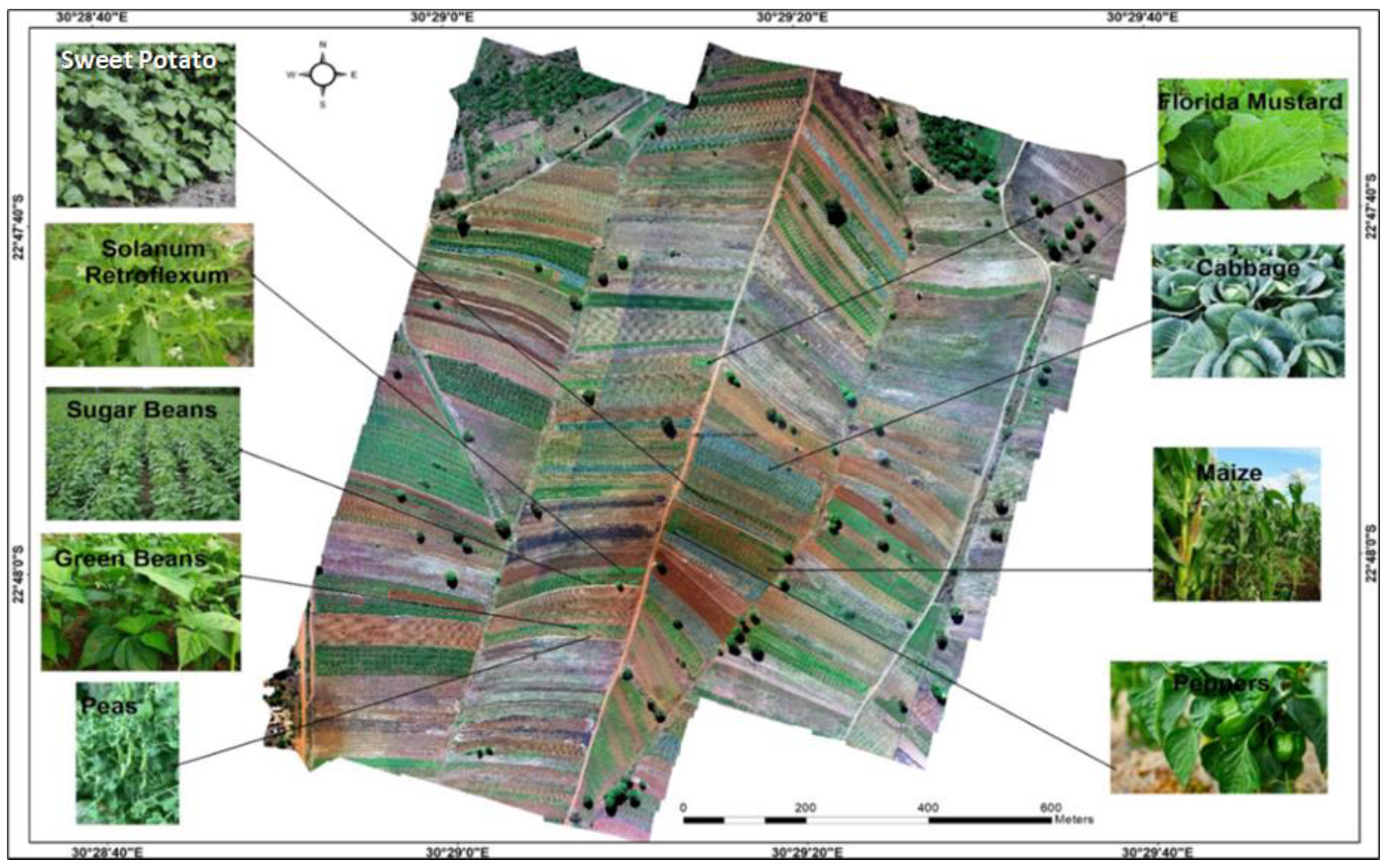
3.1. Crop Types Cultivated in the Study Area

The UAV imagery, supported by field observations, revealed a total of nine (9) different types of crops predominantly cultivated in the study area. These crop types included cabbage, maize, Florida broadleaf mustard, sweet potato, sugar beans, green beans, peas, pepper, and Solanum retroflexum. These crop types received water under the same irrigation scheduling programme, despite their differences in water requirements. Figure 3 shows the various types of crops cultivated in the study area.

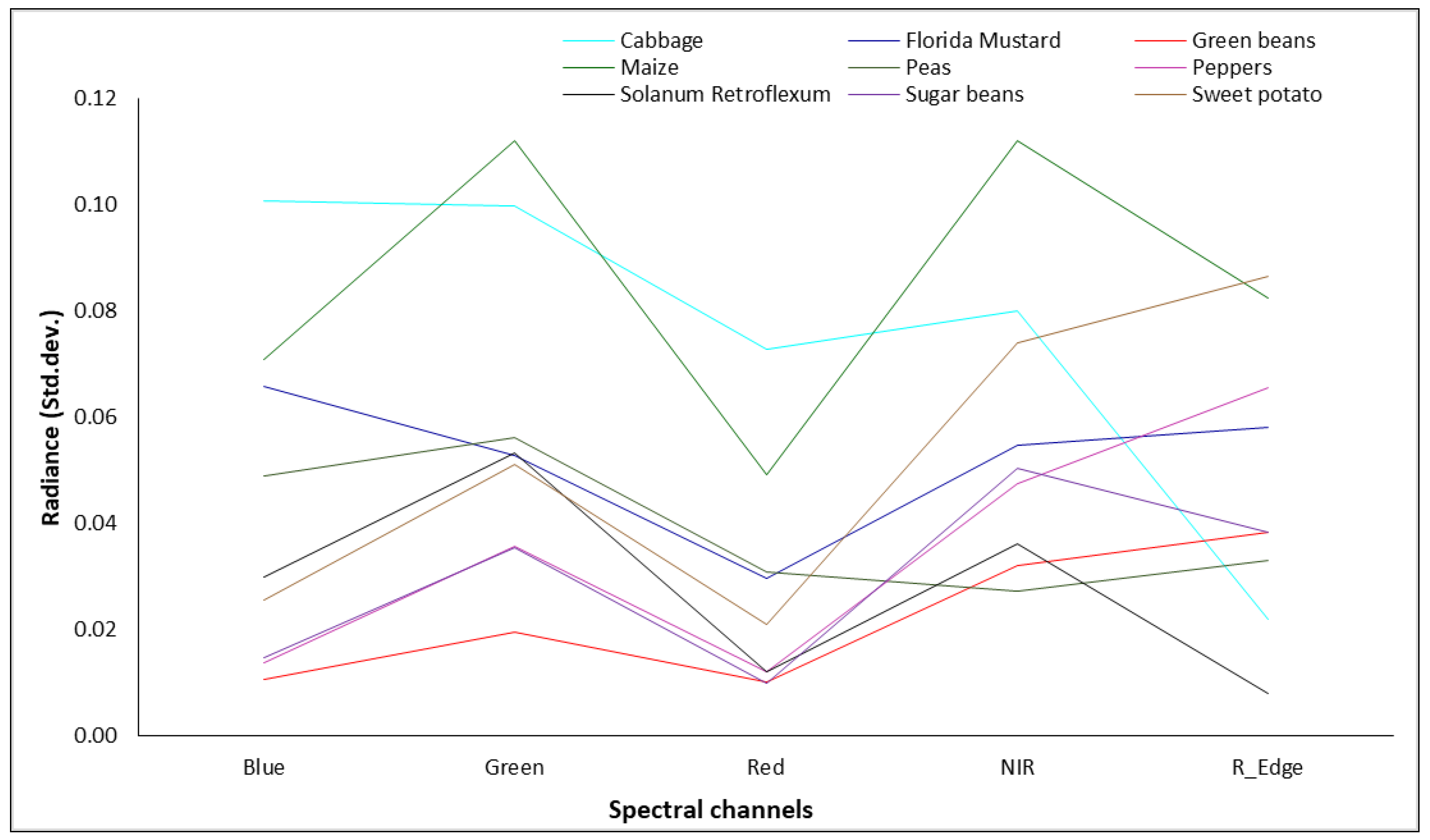
3.2. Spectral Characterization of Crops

The crops cultivated in the study area were characterized based on their spectral radiance patterns across the spectral channels of the UAV data. The main aim was to identify the spectral channel(s) suitable for characterizing a certain crop. These spectral radiance data were extracted from the visible region (blue (475 nm), green (560 nm), and red (668 nm)), red-edge region (717 nm), and near-infrared region (840 nm) of the spectrum. Figure 4 shows the spectral reflectance patterns of the cultivated crops across the spectral channels of the UAV sensor.

As seen in Figure 3, Solanum retroflexum, green beans, sweet potato, pepper, maize, and sugar beans exhibited low reflectance in the red channel and higher reflectance in the near-infrared channel of the spectrum, respectively. Peas showed low reflectance in the red channel and high reflectance in the red-edge channel of the spectrum. Cabbage exhibited low reflectance in the red channel and high reflectance in the blue channel of the spectrum. Florida broadleaf mustard exhibited low reflectance in the red channel and high reflectance in the green channel.

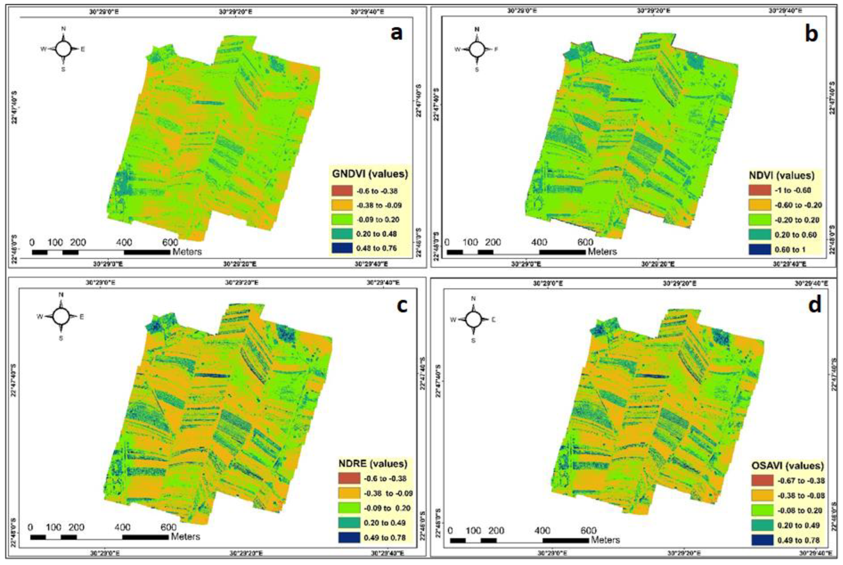
3.3. Spectral Indices for Characterizing Crop Water Content

The GNDVI, NDVI, NDRE, and OSAVI spectral vegetation indices (Figure 5) were derived from the UAV imagery to characterize different types of crops.

As seen in Figure 5a, the GNDVI shows crops with values that range between −0.7 and 0.8, with values closer to 0.8 indicating crops in good health. Figure 5b shows NDVI values that range from −0.6 to 1, with values closer to 1 indicating crops in good health. In Figure 5c, the NDRE shows crops with values that range between −0.5 and 0.7, with values closer to 0.7 indicating crops in good health. Figure 5d shows the OSAVI with values that range from −0.9 to 0.9, where values closer to 0.9 are an indication of crops in good health.

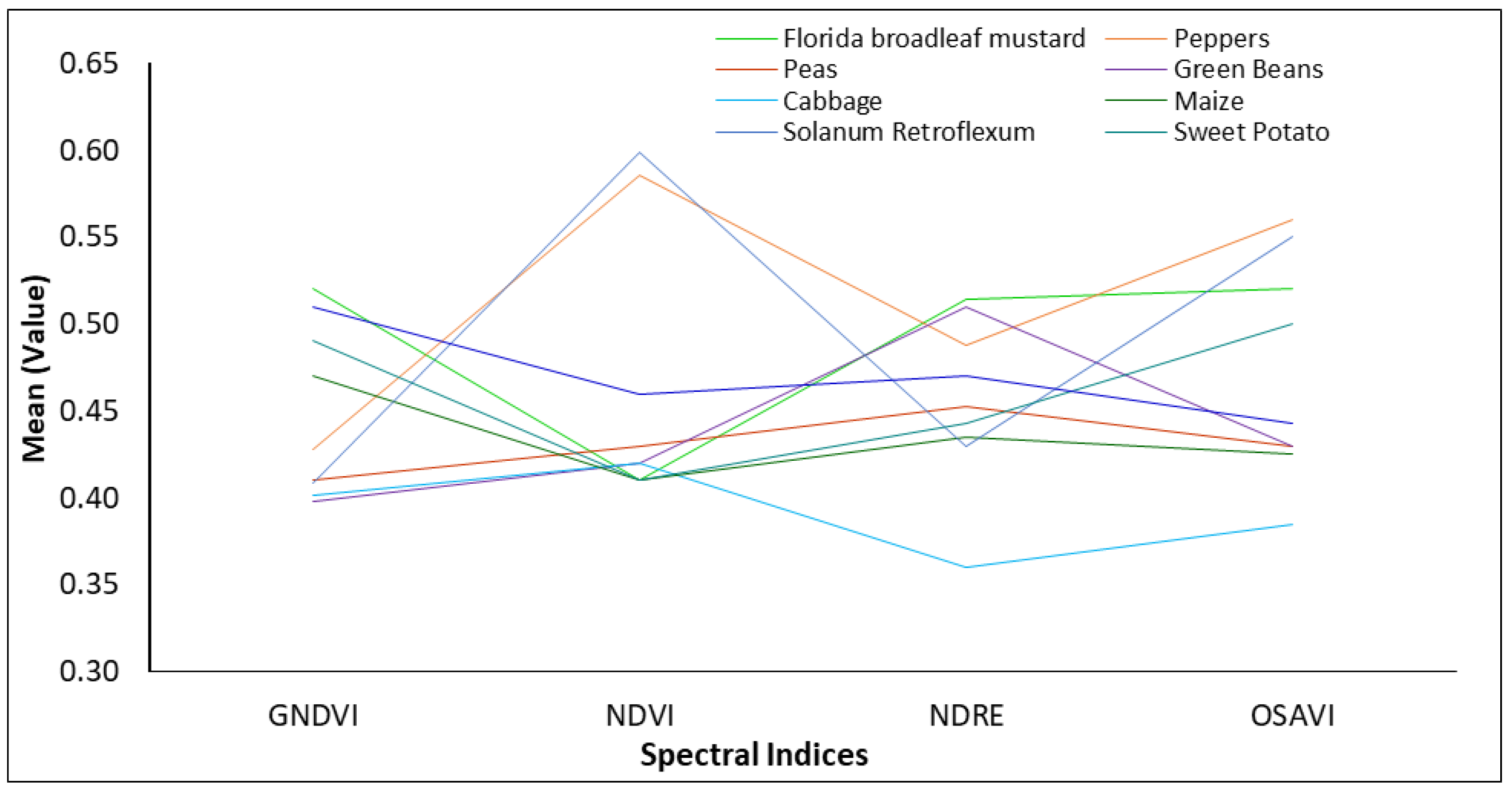
3.4. Mean Spectral Index Profile of Crops

The point shapefile containing 50 samples for each crop type was randomly digitized on the respective plots on the true colour composite (TCC) image, guided by ground truth knowledge. The point shapefile for each crop type was superimposed on each generated spectral vegetation index. The spectral vegetation index values for each sampled crop were obtained by extracting the values to the point shapefile and are presented in

Table 2. Mean spectral index values for the observed crops.

Crop Type	GNDVI	NDVI	NDRE	OSAVI
Cabbage	0.402	0.422	0.371	0.369
Maize	0.461	0.418	0.448	0.452
Florida Broadleaf Mustard	0.514	0.418	0.512	0.504
Sweet Potato	0.494	0.418	0.463	0.489
Sugar Beans	0.505	0.489	0.475	0.434
Green Beans	0.398	0.437	0.511	0.434
Peas	0.409	0.433	0.458	0.428
Pepper	0.429	0.574	0.488	0.572
Solanum retroflexum	0.411	0.594	0.439	0.590

.

Upon the successful computation of the descriptive statistics for each spectral index value for the various crops, the spectral index mean value for each crop was plotted, with a view to identifying the most suitable spectral vegetation index for each crop type. Figure 6 shows the profile of the mean values for spectral vegetation indices across various crop types in the study area.

As seen in Figure 6, according to the generated spectral vegetation indices, Solanum retroflexum, pepper, and cabbage were noted to have high spectral reflectance with the NDVI. Peas and green beans exhibited the highest spectral reflectance with the NDRE. Sweet potato, maize, sugar beans, and Florida broadleaf mustard were observed to have a high reflectance with the GNDVI. Ultimately, the OSAVI was noted to be the least accurate in terms of characterizing crops when compared with the other explored spectral vegetation indices.

Table 3. Spectral indices and their corresponding crop types.

Spectral Vegetation Index	Crop Type(s)
GNDVI	Sweet potato; maize; sugar beans; Florida broadleaf mustard
NDVI	Solanum retroflexum; pepper; cabbage
NDRE	Peas; green beans
OSAVI	-

shows the spectral indices and their corresponding crop types.

3.5. Pattern Analysis of Water Content across Surveyed Crops

Under the null hypothesis that “there was no significant variations in water content across the surveyed crops”, the Leven’s k-comparison of variance revealed insignificant differences in water content across the surveyed crops during the survey period (see

Table 4. The Levene’s k-comparison of variance results for the crop water content.

Statistics	Day 1	Day 2	Day 3
N	81	81	81
Levene’s Test Statistic	0.512	0.296	0.321
DF (categories)	8	8	8
DF Den	36	36	36
p-Value	0.839	0.963	0.953

).

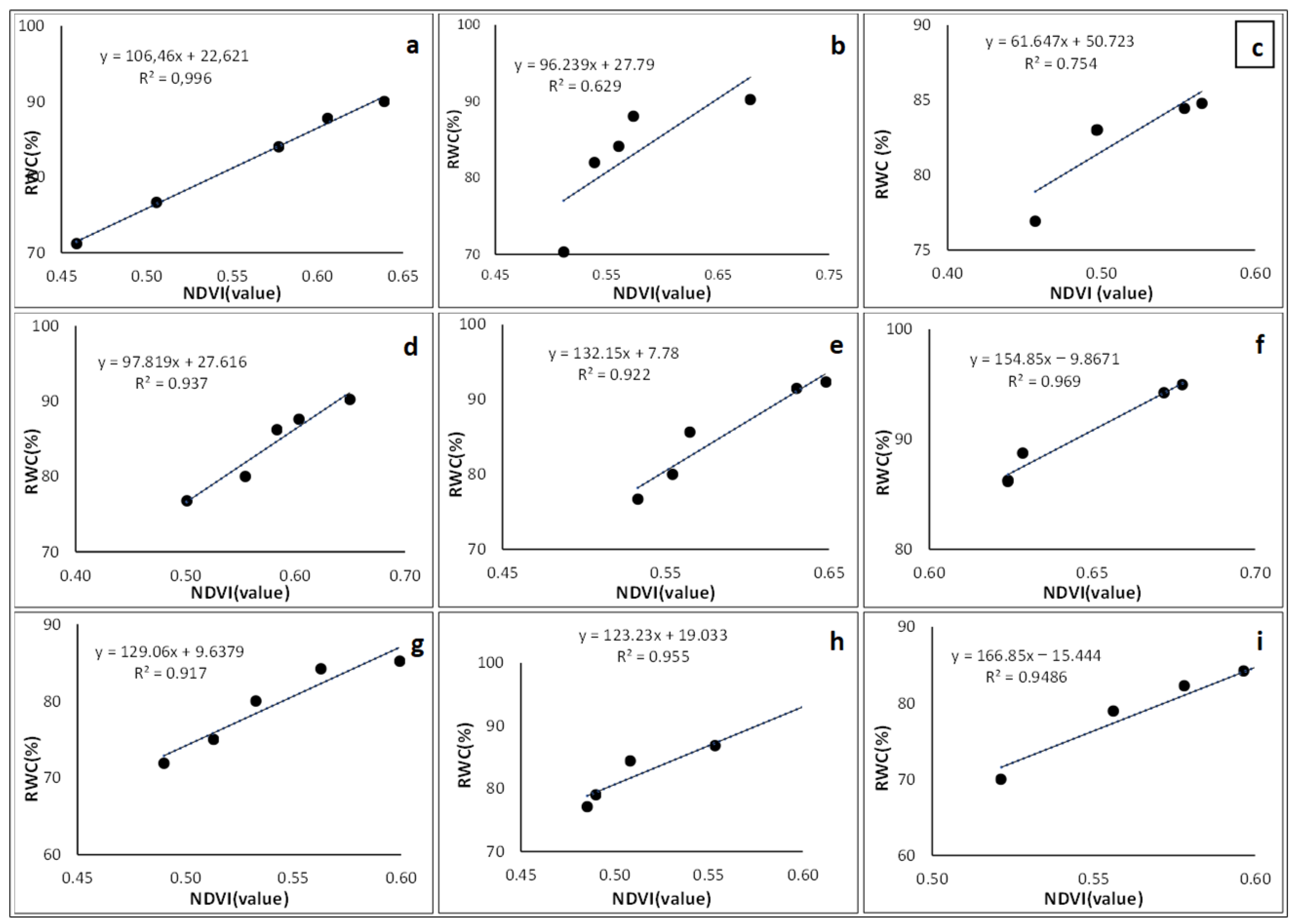
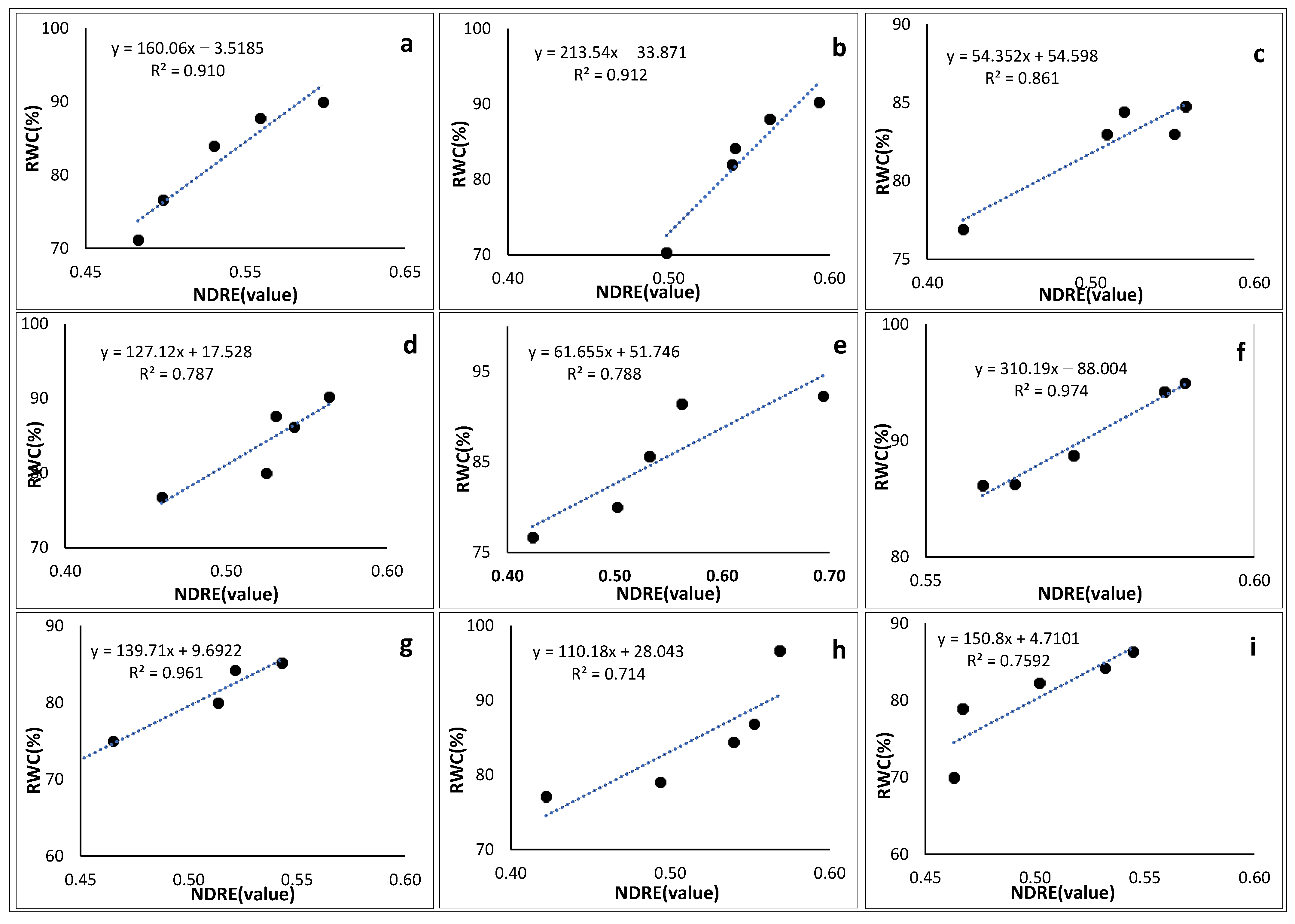
3.6. Sensitivity of Spectral Vegetation Indices to Crop Water Content

The sensitivity of several spectral indices to the water content of various crops in this study was investigated as follows.

3.6.1. Greenness Normalized Difference Vegetation Index

The linear regression analysis results reveal a significant relationship between the GNDVI and water content of eight types of crops in the study area (with r² ≥ 0.7), except for green beans (Figure 7f), with an r² value of 0.55. By implication, GNDVI can be employed to model the water content of cabbage, maize, Florida broadleaf mustard, sweet potato, sugar beans, peas, pepper, and Solanum retroflexum. Figure 7 provides the linear regression analysis results for the relationship between the GNDVI and water content of all crop types in the study area.

3.6.2. Normalized Difference Vegetation Index

The linear regression analysis results also reveal a significant relationship between the NDVI and water content of eight types of crops in the study area (with r² ≥ 0.7), except for maize (Figure 8b), with an r² value of 0.63. By implication, the NDVI can be employed to model the water content of cabbage, Florida broadleaf mustard, sweet potato, sugar beans, green beans, peas, pepper, and Solanum retroflexum. Figure 8 provides the linear regression analysis results for the relationship between the NDVI and water content of all crop types in the study area.

3.6.3. Normalized Difference Red-Edge Index

The linear regression analysis results also reveal a significant relationship between the NDRE and water content of all types of crops in the study area (with r² ≥ 0.7). Figure 9 provides the linear regression analysis results for the relationship between the NDRE and water content of all crop types in the study area.

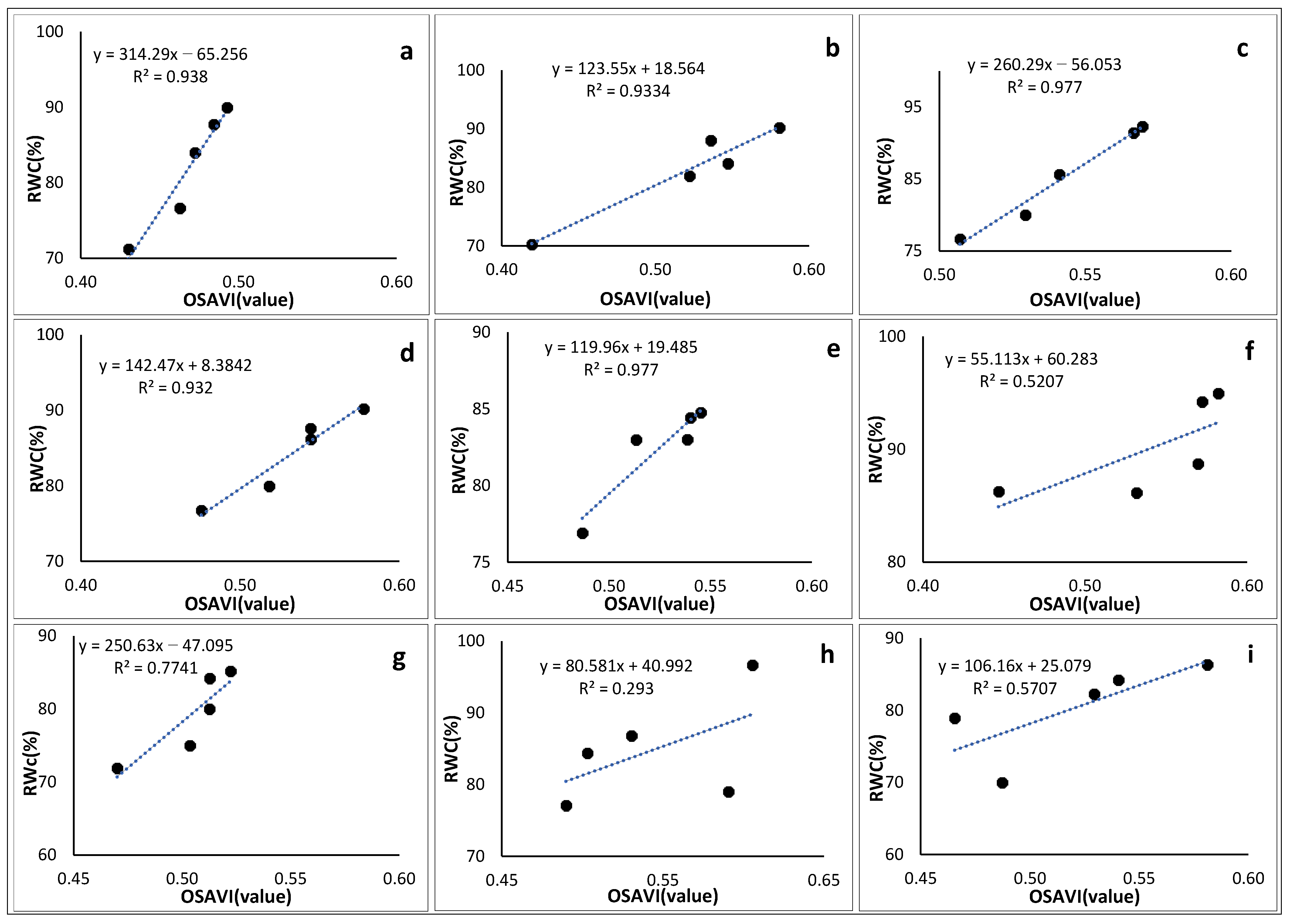
3.6.4. Optimized Soil-Adjusted Vegetation Index

The linear regression analysis results also reveal a significant relationship between the OSAVI and water content of six types of crops in the study area (with r² ≥ 0.7), except for green beans (Figure 10f), with an r² value of 0.52; pepper (Figure 10h), with an r² value of 0.29; and Solanum retroflexum (Figure 10i), with an r² value of 0.57. By implication, the OSAVI can be employed to model the water content of cabbage, maize, Florida broadleaf mustard, sweet potato, sugar beans, and peas. Figure 10 provides the linear regression analysis results for the relationship between the NDVI and water content of all crop types in the study area.

3.7. Empirical Models for Modelling Crop Water Content

Crop water content was then predicted by employing the empirical equation generated from the spectral vegetation index, which better determined the relationship with crop water content when compared with other explored spectral indices.

Table 5. Empirical models for water content.

Crop Type	Empirical Equation	r2
Solanum retroflexum	166.85 × (NDVI) − 15.444	0.949
Peas	139.71 × (NDRE) + 9.6922	0.961
Green Beans	310.19 × (NDRE) − 88.004	0.974
Sweet Potato	9.616 × (GNDVI) + 45.259	0.948
Pepper	123.23 × (NDVI) + 19.033	0.955
Cabbage	106.46 × (NDVI) + 22.621	0.996
Maize	244.89 × (GNDVI) − 51.1	0.995
Sugar Beans	205.01 × (GNDVI) − 25.4	0.978
Florida Broadleaf Mustard	88.588 × (GNDVI) + 35.805	0.953

provides the selected empirical equations based on the spectral vegetation indices that exhibited strong association with the field-measured crop water content.

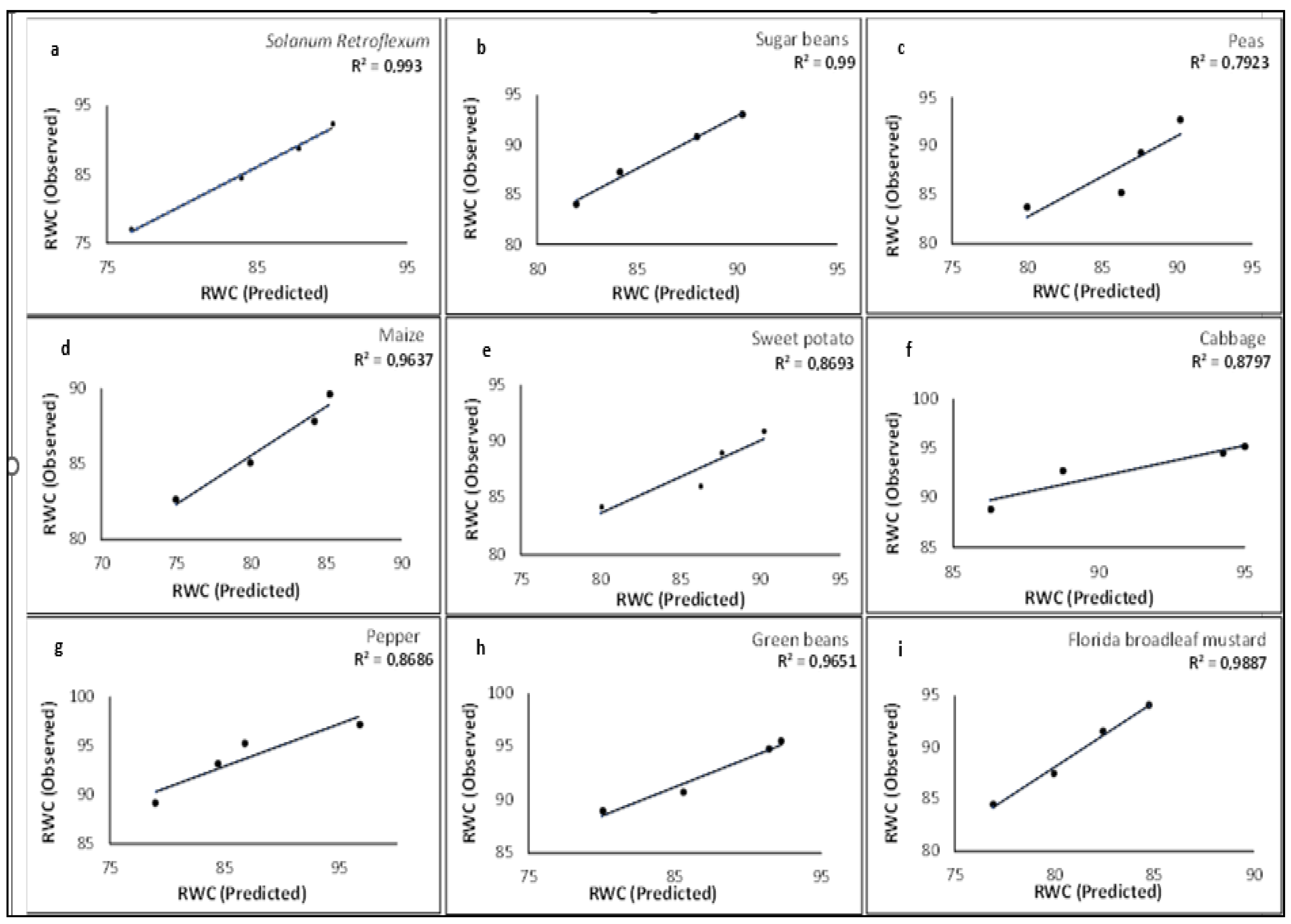
3.8. Crop Water Content Model Validation

Linear regression analysis was performed to determine the reliability of the crop water content predicted using the selected empirical models. Figure 11 provides the linear regression results explaining the performance of the selected empirical models.

The generated empirical models yielded reliable estimates of crop water content in the study area. This is evident from the r² values generated using the linear regression technique between the estimated and observed crop water content. Whereas the r² value for Solanum retroflexum, sugar beans, and Florida broadleaf mustard was noted to be 0.99 (Figure 11a,b,i), the r² values for maize and green beans was noted to be 0.96 (Figure 11d,h). Moreover, the r² value for sweet potato and cabbage was noted to be 0.86 (Figure 11e,f). Ultimately, the r² values for peas and pepper were noted to be 0.79 and 0.87, respectively. The linear regression results (Figure 11) suggest that spectral vegetation indices are capable of predicting crop water content.

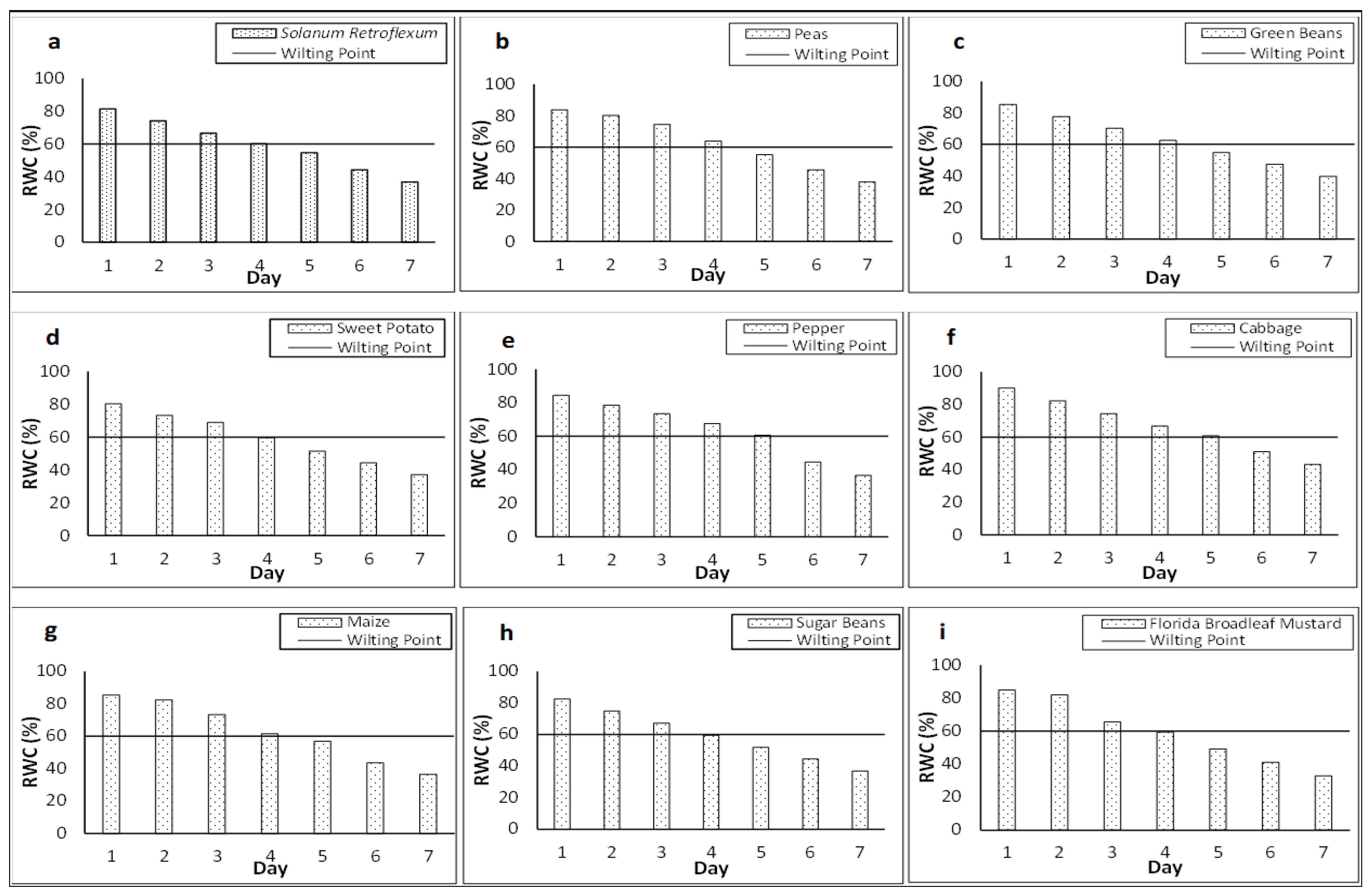
3.9. Temporal Patterns in Crop Water Content for Irrigation Scheduling

The results obtained from the time-series linear regression simulation revealed a general decline in the water content of all crops as the number of days increased. Figure 12 shows the simulated temporal changes in the water content of the crops cultivated in the study area. Forecasting was established to obtain the daily water content of the surveyed crops post-irrigation. The main purpose was to observe the number of days taken by individual crop type to reach wilting point (60% water content), a threshold point indicating the period in which a crop requires irrigation [64].

Based on the simulated patterns, Solanum retroflexum, sweet potato, maize, sugar beans, and Florida broadleaf mustard were noted to have reached their respective wilting points on day four after irrigation, as shown in Figure 11a,d,g–i, respectively. By implication, irrigation must be carried out after every four (4) days for these crops. On the other hand, peas, green beans, pepper, and cabbage were observed to have reached their respective wilting points five days after irrigation (Figure 11b,c,e,f). By implication, the irrigation of these crops should be scheduled after every five days.

4. Discussion

The importance of the timely irrigation of crops for sustainable use of water without compromising yields has long been emphasized by several studies [65,66]. However, irrigating crops equally across the entire field without considering spatial variations in soil water-holding capacity and crop water requirements may result in some sections of the field receiving an excessive amount of water and other parts experiencing water deficiency [67]. Rabiei et al. [68] noted that it is possible to devise irrigation scheduling programmes based on soil moisture data. As such, Sentinel [69] and Landsat [70] optical sensors were deemed viable for retrieving soil moisture content in agricultural lands, taking advantage of their shortwave and thermal infrared spectra. In their quest for soil moisture monitoring in agricultural lands, Zheng et al. [71] noted the feasibility of using the Sentinel-2 sensor in characterizing soil moisture, with the r² for SWIR 1 and SWIR 2 being 0.732 and 0.738, respectively. In the same study, the applicability of blue, green, red, and NIR spectral channels was tested, producing an r² of 0.191, 0.493, 0.575, and 0.600, respectively, highlighting the infeasibility of using these spectral channels in soil moisture detection. Moreover, the thermal spectral channels of the Landsat sensor can be employed to predict soil moisture content when combined with vegetation indices [72]. The relationship between TIR and the NDVI produced significant correlation coefficient values with soil moisture content [72]. However, Sishodia et al. [73] noted that it is often challenging to meet the need for monitoring crop water content at the small-scale level, due to the low spatial and temporal resolution of these sensors. Sentinel and Landsat sensors also face a challenge with respect to limited surface penetration and can easily be affected by vegetation cover [74,75,76]. To overcome these limitations, high-spatial-resolution images obtained from the UAV system were used as the base for determining crop water content, based on the visible-NIR spectrum. The UAV multispectral system was mostly preferred due to its stable data acquisition platforms and mature mosaic technology [46].

Although the reflectance in the NIR channel is mainly attributed to chlorophyll content, changes in leaf water content are known to alter chlorophyll content, which makes the visible-NIR spectrum useful for monitoring crop water [77]. The quantity of water molecules within the leaves significantly impacts solar radiation reflectance in the NIR region; as a result, the NIR region has been frequently used to assess leaf water content [48]. Therefore, spectral indices generated from the normalized ratio of NIR and red, green, and red-edge channels may provide invaluable information regarding irrigation scheduling. The in situ crop water content, in the form of RWC data, was used in this study because it permits measurements of crop leaf water content without requiring costly specialized equipment [78], unlike other field-based crop water content measurement techniques such as canopy temperature, stomatal conductance, sap flow, stem diameter variation, and leaf expansion [79,80,81]. The RWC can also be used as a diagnostic tool for determining water availability for crops [82]. The Levene’s k-comparison test enabled the assessment of spatial patterns in water content for all types of crops in the study area. The utility of this test lies in the fact that many questions in the scientific field pertain to the variances among k-populations as opposed to their means or location parameters [83].

Studies by Lugojan and Ciulca [84] and Zhang et al. [77] noted that the crop wilting point is often initiated at 60% RWC. By employing the linear regression technique, Easterday et al. [85] and Hochberg et al. [86] successfully determined the relationship between spectral vegetation indices and crop water content. Kalariva et al. [64] employed this time-series regression technique to determine the wilting point of groundnut leaves by applying the 60% RWC threshold. From a remote sensing perspective, crop types are usually characterized through image classification approaches [87]. In the current study, crop types were characterized by plotting the mean profile of their spectral radiance and spectral index values. The endmember spectral analysis results show variations in the spectral reflectance patterns of crops across the UAV spectral channels. However, a very slight difference in spectral reflectance was noted across Solanum retroflexum, green beans, sweet potato, pepper, maize, and sugar beans, as they all exhibited low and high reflectance in the red and near-infrared channels, respectively. The limited number of spectral bands in UAV imagery could be the main cause of the spectral overlaps that are commonly observed between different crop types [88]. Seeley et al. [88] also noted difficulties in crop spectral separability; this can be even more challenging when cropland contains different types of crops that are at different growing stages. The results of the study show that the spatial variability of water content across various crop types can be observed using the spectral vegetation indices maps GNDVI, NDVI, NDRE, and OSAVI. These results agree with those of Wijewardana et al. [89], who noted that the amount of water present in crop leaves shows a significant statistical correlation with leaf reflectance throughout the entire range of the electromagnetic spectrum. Ge et al. [90] noted that the highest reflectance of spectral indices was observed in healthy plants, due to there being multiple reflections of the turgid cell structure. The low spectral reflectance of the OSAVI observed in this study did not imply its unviability but the fact that there were others more sensitive to crops. With forecasting being performed for seven days in this study, it was noted that the crops generally reach their wilting points between four and five days after irrigation. Franco et al. [91] also noted that chlorophyll is very sensitive and can show significant change in a matter of a day. These results agree with those obtained by Bahadur et al. [92] and Parkash and Singh [79], who noted a significant decline in RWC when the irrigation interval was increased in tomato crops. Liu et al. [93] also noted that potato crop water content reached wilting point on the sixth day of withholding irrigation. Similarly, Ismail et al. [94] noted that water content of pepper crop reached wilting point after five days of withholding irrigation. The time-series regression simulation results obtained from this study are based on very short-term crop water patterns. As such, it must be noted that the simulation of future water patterns requires a long historical pattern. Overall, this study highlighted the significance of employing crop water content derived from spectral bands of UAV imagery in scheduling irrigation for various types of crops. However, it would be interesting to investigate the extent to which irrigation depth, soil field capacity, and soil water retention affect crop water content when devising irrigation scheduling.

5. Conclusions

This study has demonstrated the significance of devising effective irrigation scheduling programmes for various crops in small-scale farms through the modelling of crop water content patterns derived from the UAV datasets. The use of UAV datasets to meet the need for more advanced information in the agricultural sector is recommended in this study. The crop water content patterns were derived from the linear regression results between RWC and the explored spectral vegetation indices. Time-series linear regression enabled effective simulation of changes in crop water content across the various crop types. The proposed approach aimed to optimize irrigation water while preserving maximum crop yield. By using crop water content in irrigation scheduling for various types of crops, water can be saved. However, changes in crop water content were determined through temporal simulation with time-series regression. As such, it may be interesting to test these changes in the field in order to evaluate the dependability of this approach. This study also emphasized the on-going significance of remote sensing technology in addressing agricultural issues that impede hunger alleviation and food security goals. Overall, this study demonstrated winter-season crop irrigation scheduling, which may not apply for another season or geographical location due to different seasonal and environmental factors that may influence the outcome of a similar experiment.

References

1. Lowder, S.K.; Skoet, J.; Singh, S. What do We Really Know about the Number and Distribution of Farms and Family Farms in the World? Background Paper for the State of Food and Agriculture 2014; FAO: Rome, Italy, 2014. [Google Scholar]
2. Fan, S.; Rue, C. The role of smallholder farms in a changing world. In The Role of Smallholder Farms in Food and Nutrition Security; Springer: Cham, Switzerland, 2020; pp. 13–28. [Google Scholar]
3. Rapsomanikis, G. The Economic Lives of Smallholder Farmers: An Analysis Based on Household Data from Nine Countries; Food and Agriculture Organization of the United Nations: Rome, Italy, 2015; p. 48. [Google Scholar]
4. Dixon, J.; Taniguchi, K.; Wattenbach, H.; TanyeriArbur, A. Smallholders, Globalization and Policy Analysis; Food & Agriculture Organization: Rome, Italy, 2004; Volume 5. [Google Scholar]
5. Baiphethi, M.N.; Jacobs, P.T. The contribution of subsistence farming to food security in South Africa. Agrekon 2009, 48, 459–482. [Google Scholar] [CrossRef]
6. Hlophe-Ginindza, S.N.; Mpandeli, N.S. The Role of Small-Scale Farmers in Ensuring Food Security in Africa. In Food Security in Africa; IntechOpen: Rijeka, Croatia, 2021. [Google Scholar]
7. Hanjra, M.A.; Qureshi, M.E. Global water crisis and future food security in an era of climate change. Food Policy 2010, 35, 365–377. [Google Scholar] [CrossRef]
8. Booker, J.F.; Trees, W.S. Implications of Water Scarcity for Water Productivity and Farm Labor. Water 2020, 12, 308. [Google Scholar] [CrossRef] [Green Version]
9. Muzerengi, T.; Mapuranga, D. Impact of small-scale irrigation schemes in addressing food shortages in semi-arid areas: A case of Ingwizi Irrigation scheme in Mangwe District, Zimbabwe. Int. J. Humanit. Soc. Stud. 2017, 5, 298–312. [Google Scholar]
10. Lee, M.; Gambiza, J. The adoption of conservation agriculture by smallholder farmers in southern Africa: A scoping review of barriers and enablers. J. Rural. Stud. 2022, 92, 214–225. [Google Scholar] [CrossRef]
11. Beringer, T.I.M.; Lucht, W.; Schaphoff, S. Bioenergy production potential of global biomass plantations under environmental and agricultural constraints. Gcb Bioenergy 2011, 3, 299–312. [Google Scholar] [CrossRef]
12. Hussain, I.; Turral, H.; Molden, D.; Ahmad, M.U.D. Measuring and enhancing the value of agricultural water in irrigated river basins. Irrig. Sci. 2007, 25, 263–282. [Google Scholar] [CrossRef]
13. Asayehegn, K. Irrigation versus rain-fed agriculture: Driving for households’ income disparity, a study from Central Tigray, Ethiopia. Agric. Sci. Res. J. 2012, 2, 20–29. [Google Scholar]
14. Romero, R.; Muriel, J.L.; García, I.; de la Peña, D.M. Research on automatic irrigation control: State of the art and recent results. Agric. Water Manag. 2012, 114, 59–66. [Google Scholar] [CrossRef]
15. Osroosh, Y.; Peters, R.T.; Campbell, C.S.; Zhang, Q. Comparison of irrigation automation algorithms for drip-irrigated apple trees. Comput. Electron. Agric. 2016, 128, 87–99. [Google Scholar] [CrossRef] [Green Version]
16. Andrew, R.; Guan, H.; Batelaan, O. Estimation of GRACE water storage components by temporal decomposition. J. Hydrol. 2017, 552, 341–350. [Google Scholar] [CrossRef] [Green Version]
17. Babaeian, E.; Sadeghi, M.; Jones, S.B.; Montzka, C.; Vereecken, H.; Tuller, M. Ground, proximal, and satellite remote sensing of soil moisture. Rev. Geophys. 2019, 57, 530–616. [Google Scholar] [CrossRef] [Green Version]
18. Wang, H.; Li, X.; Long, H.; Xu, X.; Bao, Y. Monitoring the effects of land use and cover type changes on soil moisture using remote-sensing data: A case study in China′s Yongding River basin. Catena 2010, 82, 135–145. [Google Scholar] [CrossRef]
19. Shafian, S.; Maas, S.J. Index of Soil Moisture Using Raw Landsat Image Digital Count Data in Texas High Plains. Remote Sens. 2015, 7, 2352–2372. [Google Scholar] [CrossRef] [Green Version]
20. Przeździecki, K.; Zawadzki, J. Modification of the Land Surface Temperature–Vegetation Index Triangle Method for soil moisture condition estimation by using SYNOP reports. Ecol. Indic. 2020, 119, 106823. [Google Scholar] [CrossRef]
21. Zhang, B.; Zhao, Q.G.; Horn, R.; Baumgartl, T. Shear strength of surface soil as affected by soil bulk density and soil water content. Soil Tillage Res. 2001, 59, 97–106. [Google Scholar] [CrossRef]
22. Yang, Z.; Zhao, J.; Liu, J.; Wen, Y.; Wang, Y. Soil Moisture Retrieval Using Microwave Remote Sensing Data and a Deep Belief Network in the Naqu Region of the Tibetan Plateau. Sustainability 2021, 13, 12635. [Google Scholar] [CrossRef]
23. Deng, X.; Yang, L.; Fu, Z.; Du, C.; Lyu, H.; Cui, L.; Zhang, L.; Zhang, J.; Jia, B. A calibration-free capacitive moisture detection method for multiple soil environments. Measurement 2020, 173, 108599. [Google Scholar] [CrossRef]
24. Liu, J.; Xu, Y.; Li, H.; Guo, J. Soil Moisture Retrieval in Farmland Areas with Sentinel Multi-Source Data Based on Regression Convolutional Neural Networks. Sensors 2021, 21, 877. [Google Scholar] [CrossRef]
25. Sobrino, J.A.; Franch, B.; Mattar, C.; Jiménez-Muñoz, J.C.; Corbari, C. A method to estimate soil moisture from Airborne Hyperspectral Scanner (AHS) and ASTER data: Application to SEN2FLEX and SEN3EXP campaigns. Remote Sens. Environ. 2011, 10, 18. [Google Scholar] [CrossRef]
26. Sun, J.; Yang, L.; Yang, X.; Wei, J.; Li, L.; Guo, E.; Kong, Y. Using spectral reflectance to estimate the leaf chlorophyll content of maize inoculated with arbuscular mycorrhizal fungi under water stress. Front. Plant Sci. 2021, 12, 646173. [Google Scholar] [CrossRef] [PubMed]
27. Yue, J.; Tian, J.; Tian, Q.; Xu, K.; Xu, N. Development of soil moisture indices from differences in water absorption between shortwave-infrared bands. ISPRS J. Photogramm. Remote Sens. 2019, 154, 216–230. [Google Scholar] [CrossRef]
28. Pramudita, A.A.; Wahyu, Y.; Rizal, S.; Prasetio, M.D.; Jati, A.N.; Wulansari, R.; Ryanu, H.H. Soil Water Content Estimation With the Presence of Vegetation Using Ultra Wideband Radar-Drone. IEEE Access 2022, 10, 85213–85227. [Google Scholar] [CrossRef]
29. Homayoun, H. Remobilization of stem reserves in wheat genotypes under normal and drought stress conditions. Adv. Environ. Biol. 2011, 5, 1721–1725. [Google Scholar]
30. Bryla, D.R.; Gartung, J.L.; Strik, B.C. Evaluation of irrigation methods for highbush blueberry—I. Growth and water requirements of young plants. HortScience 2011, 46, 95–101. [Google Scholar] [CrossRef] [Green Version]
31. Lal, R.; Stewart, B.A. (Eds.) Soil-Specific Farming: Precision Agriculture; CRC Press: Boca Raton, FL, USA, 2021; p. 22. [Google Scholar]
32. Neupane, J.; Guo, W. Agronomic basis and strategies for precision water management: A review. Agronomy 2019, 9, 87. [Google Scholar] [CrossRef] [Green Version]
33. Vereecken, H.; Huisman, J.A.; Bogena, H.; Vanderborght, J.; Vrugt, J.A.; Hopmans, J.W. On the value of soil moisture measurements in vadose zone hydrology: A review. Water Resour. Res. 2008, 44, 4. [Google Scholar] [CrossRef] [Green Version]
34. Song, J.H.; Her, Y.; Yu, X.; Li, Y.; Smyth, A.; Martens-Habbena, W. Effect of information-driven irrigation scheduling on water use efficiency, nutrient leaching, greenhouse gas emission, and plant growth in South Florida. Agric. Ecosyst. Environ. 2022, 333, 107954. [Google Scholar] [CrossRef]
35. Souza, R.P.; Machado, E.C.; Silva, J.A.B.; Lagôa, A.M.M.A.; Silveira, J.A.G. Photosynthetic gas exchange, chlorophyll fluorescence and some associated metabolic changes in cowpea (Vigna unguiculata) during water stress and recovery. Environ. Exp. Bot. 2004, 51, 45–56. [Google Scholar] [CrossRef]
36. Huh, M.K.; Lee, B. The Change of Chlorophyll Content and Chlorophyll Efficiency in Epipremnum aureum by Water and pH. Eur. J. Bot. 2022, 1, 898. [Google Scholar] [CrossRef]
37. Kahil, M.T.; Connor, J.D.; Albiac, J. Efficient water management policies for irrigation adaptation to climate change in Southern Europe. Ecol. Econ. 2015, 120, 226–233. [Google Scholar] [CrossRef] [Green Version]
38. Ortega-Farias, S.; Espinoza-Meza, S.; López-Olivari, R.; Araya-Alman, M.; Carrasco-Benavides, M. Effects of different irrigation levels on plant water status, yield, fruit quality, and water productivity in a drip-irrigated blueberry orchard under Mediterranean conditions. Agric. Water Manag. 2021, 249, 106805. [Google Scholar] [CrossRef]
39. Lin, K.H.; Huang, M.Y.; Huang, W.D.; Hsu, M.H.; Yang, Z.W.; Yang, C.M. The effects of red, blue, and white light-emitting diodes on the growth, development, and edible quality of hydroponically grown lettuce (Lactuca sativa L. var. capitata). Sci. Hortic. 2013, 150, 86–91. [Google Scholar] [CrossRef]
40. Kingfield, D.M.; de Beurs, K.M. Landsat identification of tornado damage by land cover and an evaluation of damage recovery in forests. J. Appl. Meteorol. Climatol. 2017, 56, 965–987. [Google Scholar] [CrossRef]
41. Ceccato, P.; Flasse, S.; Tarantola, S.; Jacquemoud, S.; Grégoire, J.M. Detecting vegetation leaf water content using reflectance in the optical domain. Remote Sens. Environ. 2001, 77, 22–33. [Google Scholar] [CrossRef]
42. Lin, C.; Tsogt, K.; Chang, C.I. An empirical model-based method for signal restoration of SWIR in ASD field spectroradiometry. Photogramm. Eng. Remote Sens. 2012, 78, 119–127. [Google Scholar] [CrossRef]
43. Yao, J.; Wu, J.; Xiao, C.; Zhang, Z.; Li, J. The classification method study of crops remote sensing with deep learning, machine learning, and Google Earth engine. Remote Sens. 2022, 14, 2758. [Google Scholar] [CrossRef]
44. Zygielbaum, A.I.; Gitelson, A.A.; Arkebauer, T.J.; Rundquist, D.C. Non-destructive detection of water stress and estimation of relative water content in maize. Geophys. Res. Lett. 2009, 36, 1–4. [Google Scholar] [CrossRef] [Green Version]
45. Crusiol, L.G.T.; Sun, L.; Sun, Z.; Chen, R.; Wu, Y.; Ma, J.; Song, X. In-Season Monitoring of Maize Leaf Water Content Using Ground-Based and UAV-Based Hyperspectral Data. Sustainability 2022, 14, 9039. [Google Scholar] [CrossRef]
46. Zhang, L.; Zhang, H.; Niu, Y.; Han, W. Mapping Maize Water Stress Based on UAV Multispectral Remote Sensing. Remote Sens. 2019, 11, 605. [Google Scholar] [CrossRef] [Green Version]
47. Lacerdaa, L.N.; Snider, J.L.; Cohen, Y.; Liakos, V.; Gobbo, S.; Vellidis, G. Using UAV-based thermal imagery to detect crop water status variability in cotton. Smart Agric. Technol. 2022, 2, 100029. [Google Scholar] [CrossRef]
48. Ndlovu, H.S.; Odindi, J.; Sibanda, M.; Mutanga, O.; Clulow, A.; Chimonyo, V.G.P.; Mabhaudhi, T. A Comparative Estimation of Maize Leaf Water Content Using Machine Learning Techniques and Unmanned Aerial Vehicle (UAV)-Based Proximal and Remotely Sensed Data. Remote Sens. 2021, 13, 4091. [Google Scholar] [CrossRef]
49. Cai, X.; Magidi, J.; Nhamo, L.; van Koppen, B. Mapping Irrigated Areas in the Limpopo Province, South Africa; International Water Management Institute (IWMI): Colombo, Sri Lanka, 2017; Volume 172. [Google Scholar]
50. Mudzielwana, R.V.A. Analysing food security status among farmworkers in the Tshiombo Irrigation Scheme, Vhembe district, Limpopo Province (Doctoral dissertation). Agriculture 2022, 12, 999. [Google Scholar] [CrossRef]
51. Mwadzingeni, L.; Mugandani, R.; Mafongoya, P. Localized Institutional Actors and Smallholder Irrigation Scheme Performance in Limpopo Province of South Africa. Agriculture 2020, 10, 418. [Google Scholar] [CrossRef]
52. Lahiff, E.P. Agriculture and Rural Livelihoods in a South African ‘Homeland’: A Case Study from Venda; University of London, School of Oriental and African Studies: London, UK, 1997. [Google Scholar]
53. Bernal, A.; Hernández, A.; Mesa, M.; Rodríguez, O.; González, P.J.; Reyes, R. Characteristics of soil and its limiting factors of regional Murgas, Havana Province. Cultiv. Trop. 2015, 36, 30–40. [Google Scholar]
54. González, L.; González-Vilar, M. Determination of relative water content. In Handbook of Plant Ecophysiology Techniques; Springer: Dordrecht, The Netherlands, 2001; pp. 207–212. [Google Scholar]
55. Mullan, D.; Pietragalla, J. Leaf relative water content. In Physiological Breeding II: A Field Guide to Wheat Phenotyping; CIMMYT: Texcoco, Mexico, 2012; pp. 25–27. [Google Scholar]
56. Dang, L.M.; Wang, H.; Li, Y.; Min, K.; Kwak, J.T.; Lee, O.N.; Park, H.; Moon, H. Fusarium wilt of radish detection using RGB and near infrared images from Unmanned Aerial Vehicles. Remote Sens. 2020, 12, 2863. [Google Scholar] [CrossRef]
57. Filgueiras, R.; Mantovani, E.C.; Althoff, D.; Fernandes Filho, E.I.; Cunha, F.F.D. Crop NDVI monitoring based on sentinel 1. Remote Sens. 2019, 11, 1441. [Google Scholar] [CrossRef] [Green Version]
58. Mangewa, L.J.; Ndakidemi, P.A.; Alward, R.D.; Kija, H.K.; Bukombe, J.K.; Nasolwa, E.R.; Munishi, L.K. Comparative assessment of UAV and sentinel-2 NDVI and GNDVI for preliminary diagnosis of habitat conditions in Burunge wildlife management area, Tanzania. Earth 2022, 3, 769–787. [Google Scholar] [CrossRef]
59. Bastiaanssen, W.G.; Molden, D.J.; Makin, I.W. Remote sensing for irrigated agriculture: Examples from research and possible applications. Agric. Water Manag. 2000, 46, 137–155. [Google Scholar] [CrossRef]
60. Crema, A.; Boschetti, M.; Nutini, F.; Cillis, D.; Casa, R. Influence of soil properties on maize and wheat nitrogen content assessment from Sentinel-2 data. Remote Sens. 2020, 12, 2175. [Google Scholar] [CrossRef]
61. Levene, H. Robust Tests of Homogeneity of Variance. In Contributions to Probability and Statistics; Stanford University Press: Stanford, CA, USA, 1960; pp. 278–292. [Google Scholar]
62. Pierce, M.W.; Thornton, C.I.; Abt, S.R. Predicting peak outflow from breached embankment dams. J. Hydrol. Eng. 2010, 15, 338–349. [Google Scholar] [CrossRef] [Green Version]
63. Hyndman, R.J.; Athanasopoulos, G. Forecasting: Principles and Practice; OTexts: Melbourne, Australia, 2018. [Google Scholar]
64. Kalariya, K.A.; Singh, A.L.; Goswami, N.; Mehta, D.; Mahatma, M.K.; Ajay, B.C.; Chakraborty, K.; Zala, P.V.; Chaudhary, V.; Patel, C.B. Photosynthetic characteristics of peanut genotypes under excess and deficit irrigation during summer. Physiol. Mol. Biol. Plants 2015, 21, 317–327. [Google Scholar] [CrossRef] [Green Version]
65. Fan, F.; Li, B.; Zhang, W.; Porter, J.R.; Zhang, F. Evaluation of Sustainability of Irrigated Crops in Arid Regions, China. Sustainability 2021, 13, 342. [Google Scholar] [CrossRef]
66. Quimbita, W.; Toapaxi, E.; Llanos, J. Smart Irrigation System Considering Optimal Energy Management Based on Model Predictive Control (MPC). Appl. Sci. 2022, 12, 4235. [Google Scholar] [CrossRef]
67. Svedin, J.D.; Kerry, R.; Hansen, N.C.; Hopkins, B.J. Identifying Within-Field Spatial and Temporal Crop Water Stress to Conserve Irrigation Resources with Variable-Rate Irrigation. Agronomy 2021, 11, 1377. [Google Scholar] [CrossRef]
68. Yetbarek, E.; Ojha, R. Spatio-temporal variability of soil moisture in a cropped agricultural plot within the Ganga Basin, India. Agric. Water Manag. 2020, 234, 10610. [Google Scholar] [CrossRef]
69. Attarzadeh, R.; Amini, J.; Notarnicola, C.; Greifeneder, F. Synergetic Use of Sentinel-1 and Sentinel-2 Data for Soil Moisture Mapping at Plot Scale. Remote Sens. 2018, 10, 1285. [Google Scholar] [CrossRef] [Green Version]
70. Acharya, U.; Daigh, A.L.M.; Oduor, P.G. Soil Moisture Mapping with Moisture-Related Indices, OPTRAM, and an Integrated Random Forest-OPTRAM Algorithm from Landsat 8 Images. Remote Sens. 2022, 14, 3801. [Google Scholar] [CrossRef]
71. Zheng, X.; Feng, Z.; Li, L.; Li, B.; Jiang, T.; Li, X.; Li, X.; Chen, S. Simultaneously Estimating Surface Soil Moisture and Roughness of Bare Soils by Combining Optical and Radar Data. Int. J. Appl. Earth Obs. Geoinf. 2021, 100, 102345. [Google Scholar] [CrossRef]
72. Li, B.; Ti, C.; Zhao, Y.; Yan, X. Supplementary Materials: Estimating Soil Moisture with Landsat Data and its Application in Extracting the Spatial Distribution of Winter Flooded Paddies. Remote Sens. 2016, 8, 38. [Google Scholar] [CrossRef] [Green Version]
73. Sishodia, R.P.; Ray, R.L.; Singh, S.K. Applications of Remote Sensing in Precision Agriculture: A Review. Remote Sens. 2020, 12, 3136. [Google Scholar] [CrossRef]
74. Gangat, R.; van Deventer, H.; NaidooI, L.; Adam, E. Estimating soil moisture using Sentinel-1 and Sentinel-2 sensors for dryland and palustrine wetland areas. S. Afr. J. Sci. 2020, 116, 7–8. [Google Scholar] [CrossRef]
75. Rabiei, S.; Jalilvand, E.; Tajrishy, M. A Method to Estimate Surface Soil Moisture and Map the Irrigated Cropland Area Using Sentinel-1 and Sentinel-2 Data. Sustainability 2021, 13, 11355. [Google Scholar] [CrossRef]
76. Ambrosone, M.; Matese, A.; Di Gennaro, S.F.; Gioli, B.; Tudoroiu, M.; Genesio, L.; Toscano, P. Retrieving soil moisture in rainfed and irrigated fields using Sentinel-2 observations and a modified OPTRAM approach. Int. J. Appl. Earth Obs. Geoinf. 2020, 89, 102113. [Google Scholar] [CrossRef]
77. Zhang, F.; Zhou, G. Estimation of canopy water content by means of hyperspectral indices based on drought stress gradient experiments of maize in the north plain China. Remote Sens. 2015, 7, 15203–15223. [Google Scholar] [CrossRef] [Green Version]
78. Farooq, M.; Wahid, A.; Kobayashi, N.; Fujita, D.; Basra, S.M.A. Plant drought stress: Effects, mechanisms and management. Agron. Sustain. Dev. 2009, 29, 185–212. [Google Scholar] [CrossRef] [Green Version]
79. Parkash, V.; Singh, S. A Review on Potential Plant-Based Water Stress Indicators for Vegetable Crops. Sustainability 2020, 12, 3945. [Google Scholar] [CrossRef]
80. Hillel, D.; Hatfield, J.L. Encyclopedia of Soils in the Environment; Elsevier: Amsterdam, The Netherlands, 2005; Volume 3. [Google Scholar]
81. De Swaef, T.; Steppe, K.; Lemeur, R. Determining reference values for stem water potential and maximum daily trunk shrinkage in young apple trees based on plant responses to water deficit. Agric. Water Manag. 2009, 96, 541–550. [Google Scholar] [CrossRef]
82. Junttila, S.; Campos, M.; Hölttä, T.; Lindfors, L.; Issaoui, A.E.; Vastaranta, M.; Hyyppä, H.; Puttonen, E. Tree Water Status Affects Tree Branch Position. Forests 2022, 13, 728. [Google Scholar] [CrossRef]
83. Gastwirth, J.L.; Gel, Y.R.; Miao, W. The Impact of Levene’s Test of Equality of Variances on Statistical Theory and Practice. Stat. Sci. 2009, 24, 343–360. [Google Scholar] [CrossRef] [Green Version]
84. Lugojan, C.; Ciulca, S. Evaluation of relative water content in winter wheat. J. Hortic. For. Biotechnol. 2011, 15, 173–177. [Google Scholar]
85. Easterday, K.; Kislik, C.; Dawson, T.E.; Hogan, S.; Kelly, M. Remotely sensed water limitation in vegetation: Insights from an experiment with unmanned aerial vehicles (UAVs). Remote Sens. 2019, 11, 1853. [Google Scholar] [CrossRef] [Green Version]
86. Hochberg, U.; Bonel, A.G.; David-Schwartz, R.; Degu, A.; Fait, A.; Cochard, H.; Peterlunger, E.; Herrera, J.C. Grapevine acclimation to water deficit: The adjustment of stomatal and hydraulic conductance differs from petiole embolism vulnerability. Plants 2017, 245, 1091–1104. [Google Scholar] [CrossRef]
87. Orynbaikyzy, A.; Gessner, U.; Mack, B.; Conrad, C. Crop Type Classification Using Fusion of Sentinel-1 and Sentinel-2 Data: Assessing the Impact of Feature Selection, Optical Data Availability, and Parcel Sizes on the Accuracies. Remote Sens. 2020, 12, 2779. [Google Scholar] [CrossRef]
88. Seeley, M.M.; Martin, R.E.; Vaughn, N.R.; Thompson, D.R.; Dai, J.; Asner, G.P. Quantifying the variation in refectance spectra of Metrosideros polymorpha canopies across environmental gradients. Remote Sens. 2023, 15, 1614. [Google Scholar] [CrossRef]
89. Wijewardana, C.; Alsajri, F.A.; Irby, J.T.; Krutz, L.J.; Golden, B.; Henry, W.B.; Gao, W.; Reddy, K.R. Physiological assessment of water deficit in soybean using midday leaf water potential and spectral features. J. Plant Interact. 2019, 1, 533–543. [Google Scholar] [CrossRef] [Green Version]
90. Ge, X.; Wang, J.; Ding, J.; Cao, X.; Zhang, Z.; Liu, J.; Li, X. Combining UAV-based hyperspectral imagery and machine learning algorithms for soil moisture content monitoring. PeerJ. 2019, 7, 6926. [Google Scholar] [CrossRef]
91. Franco, A.C.; Haag-Kerwer, A.; Herzog, B.; Grams, T.E.E.; Ball, E.; de Mattos, E.A.; Scarano, F.R.; Barreto, S.; Garcia, M.A.; Mantovani, A.; et al. The effect of light levels on daily patterns of chlorophyll fluorescence and organic acid accumulation in the tropical CAM Treeclusia Hilariana. Trees 1996, 10, 359–365. [Google Scholar] [CrossRef]
92. Bahadur, A.; Lama, T.D.; Chaurasia, S.N.S. Gas exchange, chlorophyll fluorescence, biomass production, water use and yield response of tomato (Solanum lycopersicum) grown under deficit irrigation and varying nitrogen levels. Indian J. Agric. Sci. 2015, 85, 224–228. [Google Scholar]
93. Liu, F.; Shahnazari, A.; Andersen, M.N.; Jacobsen, S.E.; Jensen, C.R. Effects of deficit irrigation (DI) and partial root drying (PRD) on gas exchange, biomass partitioning, and water use efficiency in potato. Sci. Hortic. 2006, 109, 113–117. [Google Scholar] [CrossRef]
94. Ismail, M.R.; Davies, W.J.; Awad, M.H. Leaf growth and stomatal sensitivity to ABA in droughted pepper plants. Sci. Hortic. 2002, 96, 313–327. [Google Scholar] [CrossRef]
Figure 1. The location of the study area.
Sustainability 15 12034 g001
Figure 2. Overview of the UAV equipment: (a) the DJI Matrice 600 (M600) UAV system; (b) Micasense RedEdge multispectral camera; and (c) the Micasense Calibrated Reflectance Panel.
Sustainability 15 12034 g002
Figure 3. Crop types cultivated in the study area.
Sustainability 15 12034 g003
Figure 4. Spectral behaviour of the observed crops.
Sustainability 15 12034 g004
Figure 5. (a) GNDVI, (b) NDVI, (c) NDRE, and (d) OSAVI.
Sustainability 15 12034 g005
Figure 6. Mean spectral values of vegetation indices for various crops.
Sustainability 15 12034 g006
Figure 7. Linear regression analysis results for GNDVI–crop water content relationship ((a), Florida mustard (b) maize, (c) cabbage, (d) sweet potato, (e) sugar beans, (f) green beans, (g) peas, (h) pepper, and (i) solanum Retroflexum).
Sustainability 15 12034 g007
Figure 8. Linear regression analysis results for NDVI–crop water content relationship ((a), Florida mustard (b) maize, (c) cabbage, (d) sweet potato, (e) sugar beans, (f) green beans, (g) peas, (h) pepper and, (i) solanum Retroflexum).
Sustainability 15 12034 g008
Figure 9. Linear regression analysis results for NDRE–crop water content relationship ((a), Florida mustard (b) maize, (c) cabbage, (d) sweet potato, (e) sugar beans, (f) green beans, (g) peas, (h) pepper, and (i) solanum Retroflexum).
Sustainability 15 12034 g009
Figure 10. Linear regression analysis results for OSAVI–crop water content relationship ((a), Florida mustard (b) maize, (c) cabbage, (d) sweet potato, (e) sugar beans, (f) green beans, (g) peas, (h) pepper, and (i) solanum Retroflexum).
Sustainability 15 12034 g010
Figure 11. Scatterplot graph explaining the reliability of the selected empirical models ((a) Solanum Retroflexum, (b) sugar beans, (c) peas, (d) maize, (e) sweet potato, (f) cabbage, (g) pepper, (h) green beans, and (i) Florida broadleaf mustard).
Sustainability 15 12034 g011
Figure 12. Simulated temporal patterns in water content across the surveyed crops ((a) solanum Retroflexum, (b) peas, (c) green beans, (d) sweet potato, (e) pepper, (f) cabbage, (g) maize, (h) sugar beans, and (i) Florida broadleaf mustard).
Sustainability 15 12034 g012