Article

System Dynamics and Sustainable Solution: The Case in a Large-Scale Pallet Manufacturing Company

by
Ernesto A. Lagarda-Leyva
,
María Paz Guadalupe Acosta-Quintana
,
Javier Portugal-Vásquez
,
Arnulfo A. Naranjo-Flores
and
Alfredo Bueno-Solano
*
Industrial Engineering Department, Instituto Tecnológico de Sonora, Cd Obregón 85000, Mexico
*
Author to whom correspondence should be addressed.
Sustainability 2023, 15(15), 11766; https://doi.org/10.3390/su151511766
Submission received: 31 May 2023 / Revised: 7 July 2023 / Accepted: 24 July 2023 / Published: 31 July 2023
(This article belongs to the Special Issue Business Models and Innovation for Sustainability Transition)

Abstract

:
The proposal in the present research study is the result of a more than two-year process developed in a pallet manufacturing company for anchor enterprises in Southern Sonora, Mexico dedicated to beer production and export to the United States of America. Considering the high pallet demand for this supplier, a strategic plan was created in 2021, establishing an important project for developing technological solutions to improve decision making supported by graphical user interface and focused on sustainability. This study shows the application of system dynamics in all the wood and pallet manufacturing processes with a strategic sourcing supply chain. The method used for its development had the following stages: (1) developing the mapping process; (2) creating the causal loop diagram; (3) developing a flow and stock model with the representing mathematical equations; (4) simulating and validating current scenarios; (5) evaluating normal, optimistic, and pessimistic scenarios with multicriteria decision making using Technique to Order Preferences by Similarity and the Ideal Solution (TOPSIS) and Faire Un Choix Adéquat (FUCA); (6) building the graphical interface. The most relevant results for the company were having quantitative information regarding the pallet demand required by the main client for wood availability, which was the main restriction in the supply chain. The solution was based on four validation tests that allowed decision makers to support the production proposals considering the assistance of the dynamic models. The main conclusion demonstrated that using well-defined operation rules and policies—considering the installed capacity and pallet demand through the model solution—allows anticipating decisions on pallet quantity and reducing the risk of out-of-time deliveries.

1. Introduction

Developing suppliers is an important aspect for enterprises that depend on response time and product quality. Suppliers have turned out to be critical elements for organizations since they are the persons responsible for providing on-time materials and services [1]. They are part of the supply chain that provides the production link and allows evaluating decisions between the interactions generated in this first client–supplier internal relationship [2]. In this sense, when evaluating and selecting suppliers, the objectives of the organization should be coordinated and an eye kept on quality standards, costs, and delivery time, among other variables. Thus, robust methodologies capable of managing such complexities are needed. For this purpose, the system dynamics methodology enabled simulating complex systems from different operational rules and policies [3,4,5,6]. Therefore, causal models were constructed based on the systematic thought theory.

Literature Review

The causal diagrams analyzed the cause–effect relationships between the variables that conformed the model with behaviors denominated as reinforcement (R) and balance (B). These models helped to know the different connected loops that create, on the one hand, mental models and, on the other hand, simulation models to understand the systematic thought complexity and to obtain the conclusions from data and decision making [7].
Likewise, the simulation model was developed in Stella® Architect—a simulator that uses solution algorithms of differential equations—based on Chapra and Canale [8], using Euler’s and Runge–Kutta methods. Subsequently, the model validation was performed, considering the proposals of Kleinjen [9] and Barlas and Carpenter [10]. With these proposals, the sensitivity analysis generated the different scenarios in situations evaluated by time and analyzed from the perspective of pessimistic and optimistic behaviors from the current scenario given by the response of the model initially implemented [11].
The scenarios required the selection of the most critical variables to apply a multicriteria decision-making (MCDM) analysis considering two techniques: (1) Technique to Order Preferences by Similarity and the Ideal Solution (TOPSIS) and (2) Faire Un Choix Adéquat (FUCA) developed by Fernando et al. [12] and Wang and Rangaiah [13]. The results of both techniques were 15 scenarios, classified in 5 current, 5 pessimistic, and 5 optimistic scenarios for decision making based on data.
Saha et al. [14] used mathematical models and algorithms to determine the optimal rate of investment in technology of green preservation and dynamic investment strategy for waste reduction. The present research study shows a production proposal of pallets distributed to a beer company. The dynamics system models included multicriteria techniques as part of their procedure for selecting the best scenario from the optimization criteria in the following variables: wood storage, wood with fungus, clean wood, pallet warehouse inventory, sawdust inventory total pallets for clients, and cash inflows.
Given the complexity of the existing mathematical models, as well as the nomenclature used in the development of the solutions, the graphical user interface generated a more adequate understanding and interactions between the user and the computer [15,16].
The present study was developed in a pallet manufacturing company with an average volume of 38,000 pallets/month to supply a beer company from Southern Sonora, Mexico, which produces and distributes to the United States of America in great volumes. In 2021, a strategic planning exercise was developed, integrating three pallet manufacturing companies into the project. The 2021–2026 strategic planning exercise developed by Lagarda Leyva and Zavala [17] generated a strategic map, where the objective in the process perspective was defined as technological solutions for improving decision making in complex environments.
As a result of this effort, and to give a response to the strategic objective, the project of developing a technological solution was performed in 2021 based on a graphical user interface and the system dynamics methodology proposed by Forrester and Sterman [18,19]. The decision makers’ interest was to have a model that allowed balancing planning and managing the responsible acquisition of raw matter and minimizing the risks [20]. Thus, the current production capacity and future needs of investment were measured to meet the daily pallet demand and the requirements of the mega Southern Sonora beer producer for export to the USA.
Diverse investigations have used the Data Science (DS) approach to analyze the behavior of the inventories facing disruptive events and their propagation in the network. Different empirical studies have been developed with simulations to evaluate the pallet supply chain behavior. Among those that stand out are Gnoni et al. [21], who developed a simulation model to compare scenarios in terms of time of the provider service and internal and global operation costs. The results confirmed that better coordination of the reverse chain agents increased the yield of all the systems.
On the other hand, Valerio and Gnoni [22] studied the behavior of the feedback loops generated in the pallet supply chain. Their objective was to describe the critical factor in a pallet logistic network or exchange system, using a causal diagram and developing a tool based on simulation to help the logistic agents and to design efficient organizational scenarios for these systems.
Newman et al. [23] developed a simulation model in experimental conditions that included variability levels of demand, quantity of pallets available for the system, incremental load time, and rejection rate when pallets of general usage were made. In the majority of cases, their results indicated a significant system yield increase with pallets of general usage, except for the incremental load time and waste rates associated with pallet assemblage, which were higher.
Dynamics systems evaluate the effect of inventory delays that happen in the supply chain where the dependence from one link to the other is given. For example, starting from the materials, transformation processes and deliveries to clients should comply with delivery time to maintain the expected inventories. Nabil [24] set out this dependence through system dynamics for different operational conditions with a manufacturing simulation model that comprised a quality control unit, which was also a system bottleneck. Therefore, the size of the optimum lot was demonstrated, giving place to a minimum delivery time and whose level of optimum inventory agreed with the one expected.
The main contributions set up previously for each of the authors may be expressed, as shown in Table 1.

2. Materials and Methods

The materials used in this study were (1) Vensim PLE® (Versión 8.2.1, Ventana System Inc., Harvard, MA, USA, 2019) to draw loops B and R; (2) Stella® Architect, 2023 (Version 3.3, Isee Systems Inc., Lebanon, NH, USA, 2023) to build the flow and stock diagrams, simulations; GUI. These software were selected because they included the module to design the graphical user interface with the pallet producers. (3) Excel® (Microsoft, Redmond, WA, USA, 2018) was used for processing data and information (TOPSIS and FUCA).

2.1. System Dynamics Stage

The method used to develop the technological solution considered the five stages described as follows [3,4,5,29]:
Mapping the pallet factory supply chain. The system approach was used to analyze each one of the pallet manufacturing process links in general. The result generated was a diagram observing the client–provider relationships in the supply chain and considering wood provision (stock), pallet production, and delivery to clients, as well as aspects related to waste reassessment (reverse logistics).
Developing the causal loops diagrams. Taking mapping the pallet supply chain as a reference, an analysis of the cause–effect relationships was carried out, classified as reinforcer (R) and balance (B) loops to understand the complexity of all the manufacturing processes and deliveries from the system dynamics perspective.
Developing the flow and level diagram with the mathematical equations that represent them. For the diagram construction, Stella® Architect software, version 3.3 was used considering all the model parameters from the relationships between them. The mathematical equations that totally represented the system behavior were constructed.
Simulating and validating the current scenario. Likewise, the simulation was made from the current pallet manufacturing conditions. The average error validation techniques were used from the production reality versus the solution offered by the model.
Building a graphical interface. This was the last step where the technological solution in an environment was concentrated, where the decision maker can incorporate input data to the model and execute it for decision making in the pallet supply chain.

2.2. Multicriteria Decision Making

After creating the dynamics model, three scenario categories were considered: current, optimistic, and pessimistic. Each scenario, when executed, considered the following parameters as variation methods: (a) delivery time of wooden pallets; (b) delivery time of pallets to the final customer; (c) price per pallet according to demands. All these values were modified according to the scenarios executed. In the case of the current scenario, the selected values were those that the company provided at the moment of developing the solution; in the pessimistic scenario, these parameters of the same three indicators were considered as the ones that would put the organization at risk, that is, in terms of the same three parameters rising considerably. Finally, in the optimistic scenario, the three same parameters were considered improved to put the organization in the ideal situation to cover the commitments with the main client.
Each one of these scenarios considered 5 alternatives; thus, 15 alternatives were taken into account and evaluated by the following criteria, the same that were validated by the organization from the following 8 variables that were considered in the process analysis of the scenarios in the FUCA and TOPSIS methods, with the optimization criteria and weighting value assigned by the company:
  • WS—wood storage (units); refers to the quantity of wood available in the organization coming mainly from Mexico cut into pieces in the measurements required for the pallets.
  • WF—wood with fungus (units); considered as a high risk if assembled as pallets due to the effect of the humidity captured during transportation, since the pallet may reach its destination with fungi due to its sensitivity. Upon arrival, wood is treated with an established cleaning process by the company.
  • WC—wood clean (units). Clean wood refers to the total quantity of wood ready to be assembled to make the pallets.
  • AP—the pallets assembled from the wooden pieces required for their production.
  • IPW—inventory in the pallet warehouse (units); refers to the inventory of the pallets generated and stored in the warehouse for its distribution.
  • SI—sawdust inventory (tons); refers to the quantity of sawdust generated as part of the planning process of the wooden pieces, which represents a loss but that is used and sold as a secondary product.
  • TPC—total pallets per client (units); refers to the total quantity of pallets assigned to the clients of the organization.
  • CI—cash inflow (MXN); refers to the daily money income in the organization, of which the production cost has been deducted (data not available because of confidentiality); thus, the sale price generates the organization utility.
The next step was necessary to define pesos/weighting to calculate each of the criteria (i.e., its degree of importance) and to define the objective to be reached (maximize or minimize). Then, the variables were listed, with weighting in parenthesis: minimize WS (10%); minimize WF (10%); maximize WC (15%); maximize AP (15%); minimize IPW (10%); minimize SI (5%); maximize TPC (15%); maximize CI (20%)
Once the previous information was defined, a decision matrix was created, such as the one shown in Table 2.
Finally, MCDM techniques were used to rank the alternative. The techniques selected were TOPSIS and FUCA because they were easy to use and have demonstrated good performance in solving matrixes with considerable criteria [30]; furthermore, both methods are widely used in diverse research environments [31,32,33,34]. It is important to highlight that the description of the methods is beyond the reach of this research study.

3. Results

The results are presented below, considering the six steps of the proposed procedure.

3.1. Mapping the Supply Chain of Pallet Manufacturing

In general, Figure 1 shows the pallet supply chain where each stage is explained separately.
The links in Figure 1 are explained as follows:
Supply. The supply starts with wood provision for the sawmills (in the states of Durango, Chihuahua, Sonora, and Sinaloa), mainly from the massive pine tree forests. The wood is transported in different forms toward the warehouses of the different pallet manufacturers. All the sawmills should have the commitment of reforesting in conjunction with official entities (1, 2, 3, 4, 11).
Production. Each manufacturer independently runs its internal processes according to personnel, physical infrastructure, and available equipment, as well as the human resources assigned according to expertise and performance in the tasks assigned (4, 5, 6, 7, 9, 11). All the manufacturers—as previously mentioned—should be committed to reforest jointly with the official entities.
Finished product distribution. The pallets are set up in the different transportation modes used by each of the manufacturers and placed in the final client warehouse (6, 7, 8).
Final client. The main customer that has been analyzed is the brewery company, based on the scheduled demands of pallets; according to the orders, the production process is established, generating income for the organization from the entries (8, 9, 11). The clients must promote the behavior of reforesting in conjunction with official entities and their providers.
Reverse logistics. This stage takes place in each pallet factory when wood cannot be exploited to make pallets, such as waste generated (sawdust and profile wood, among others). In the same manner, pallets are recycled and placed as second-hand products for a certain type of client (10, 11) (achieved by the main wood used as raw matter for pallet manufacturing).

3.2. Creating the Causal Diagram from the Dynamics Hypotheses

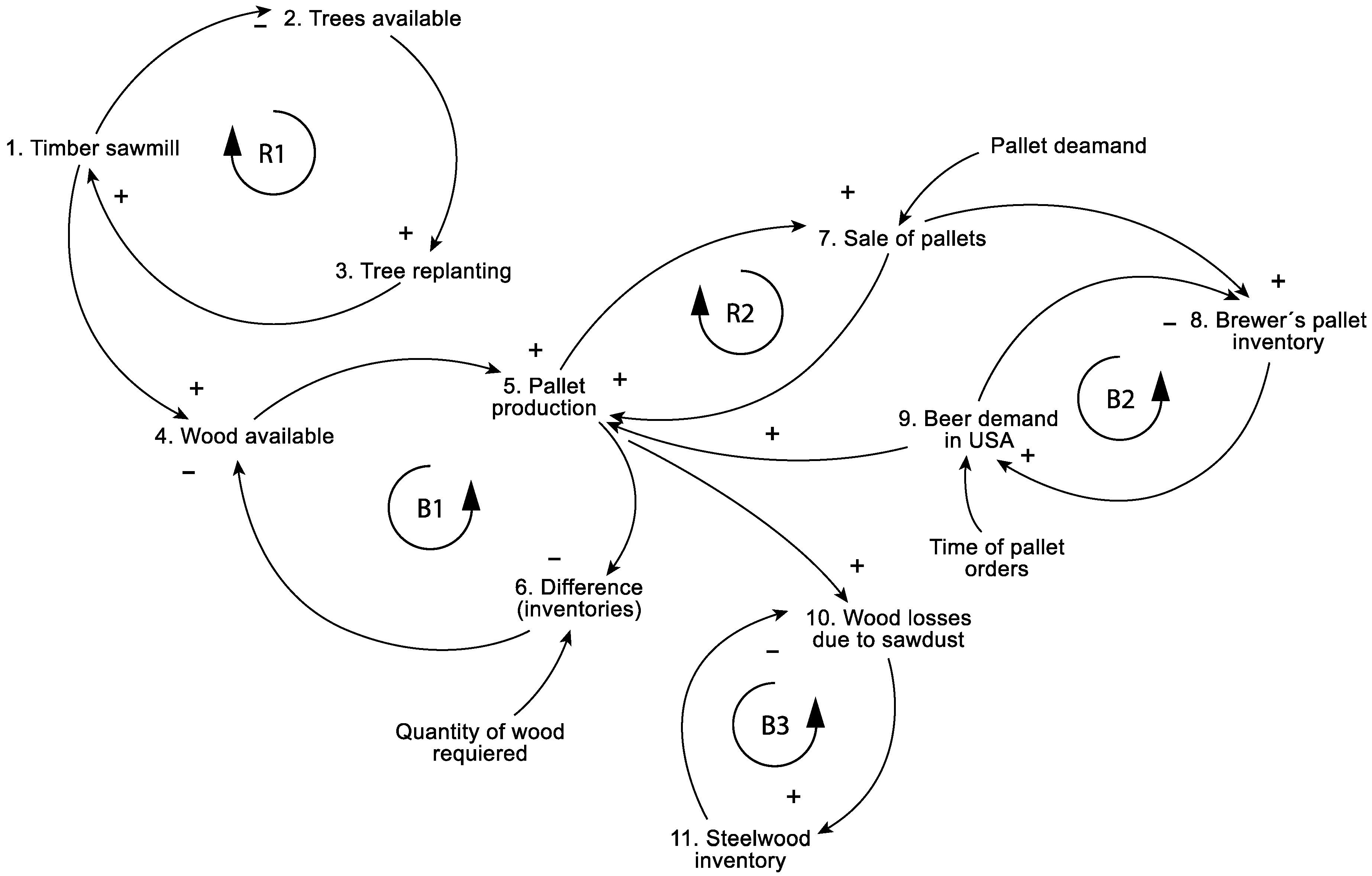
A dynamics hypothesis allows generating the idea that the causal diagram structure could communicate in terms of its dynamic behavior associated with the variables of the analysis from the existing relationships, among them Sterman [19]. Considering the previous mapping of the supply chain, the causal diagram was developed, as shown in Figure 2, where the type B and R loops can be observed from the three dynamics hypotheses as follows:
  • Hd1: the wood for pallet construction depends on availability and permits to cut pine trees in the cities that offer this product;
  • Hd2: the amount of pellet production depends on the final client from the operation rules of 30% assigned only for the local supplier;
  • The wooden quantity in the inventory depends on the pallet demand to ship beer to the final client.
The diagram shows three reinforcing (R1, R2, R3) and three balance (B1, B2, B3) loops.
The reinforcing R1 (1→2→3→1) loops’ dynamics can be explained as follows: the more sawmills that exist, the more that uncontrolled tree felling reduces wood availability per available tree, which implies trees replanting per each eliminated tree so that sawmills continue producing wood.
The B1 (4→5→6→4) loops expose in their dynamics that the more wood there is available the greater pallet production is allowed. According to a dynamics inventory, the difference is reduced because the warehouse is full with the required amount, reducing the input of the available wood to the production process.
The reinforcing R2 (5→7→5) loops establish that greater pallet production depends on demand and sales grow in the time required to maintain high pallet production levels.
The reinforcer B2 (8→9→8) loop is represented by the pallet inventory growth dynamic variables delivered to the final client by the effect of the high beer consumption demand in the USA, which in time reduces the pallet inventories.
The reinforcing B3 (10→11→10) loops are composed of dynamic wood reduction (sawdust) variables due to the effect of high pallet production, which in time increases sawdust inventories.

3.3. Creating Flow and Level Diagrams with the Model Equations

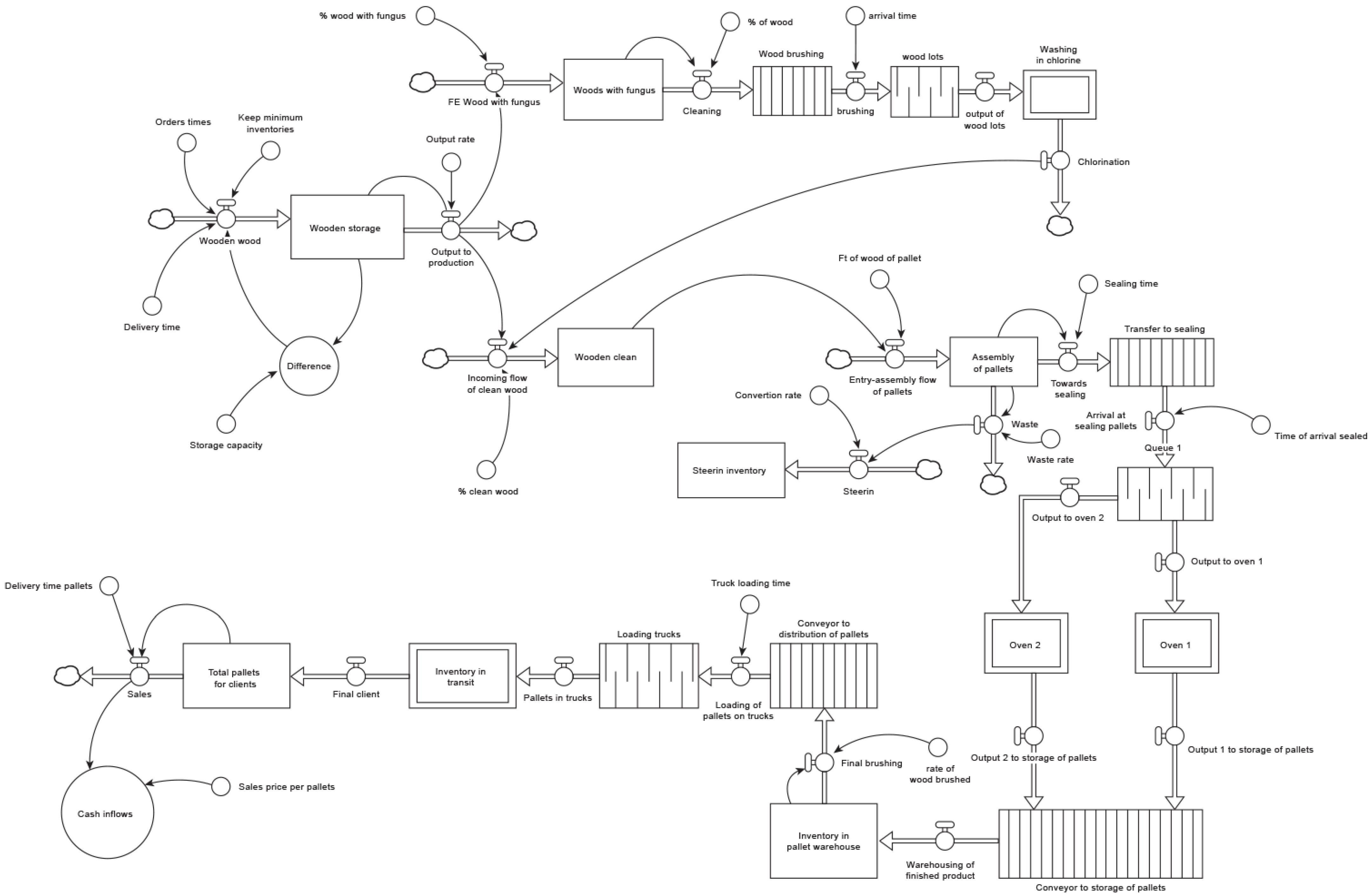
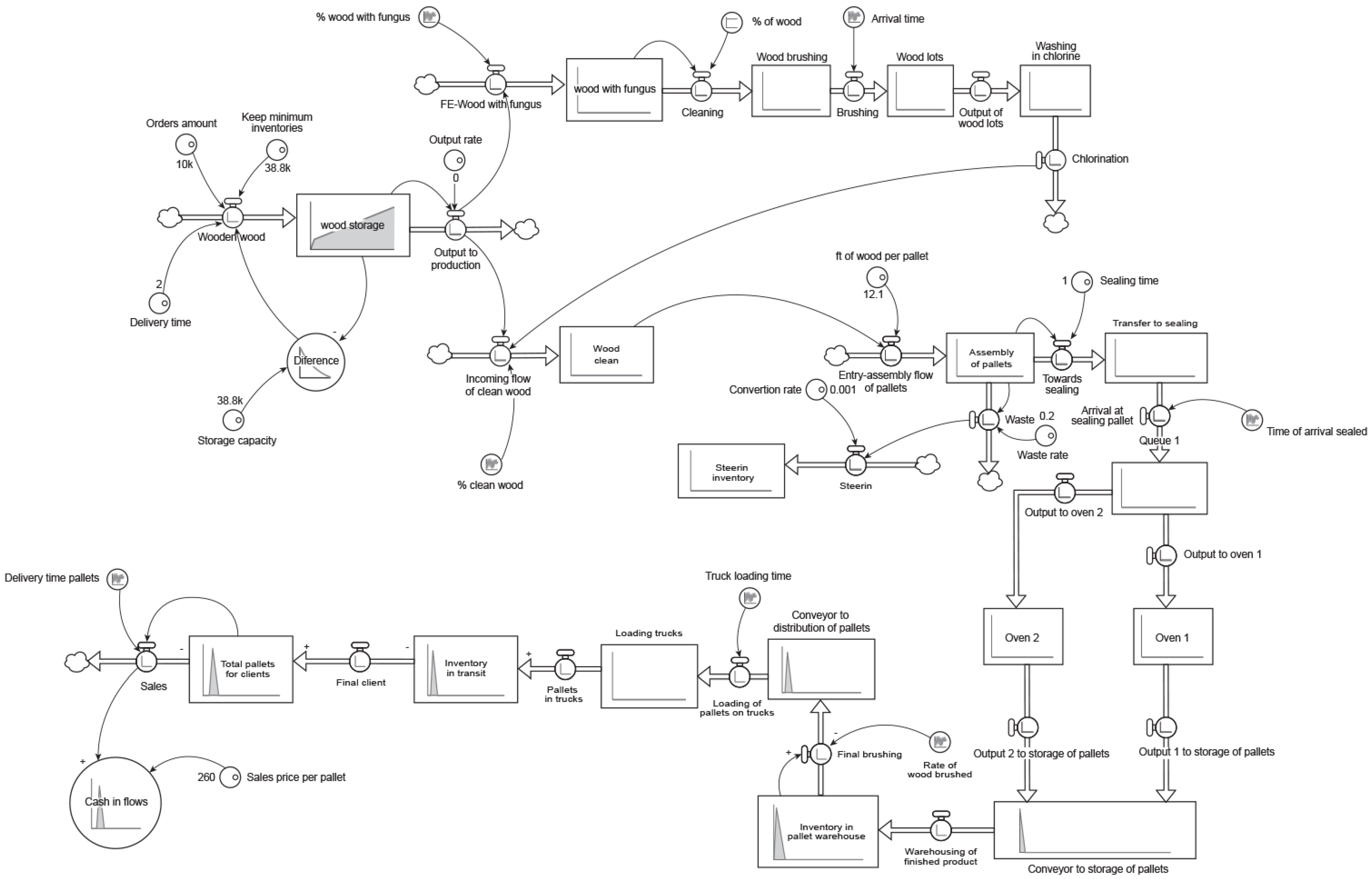
The flow and level diagram was created from the logics of the supply chain operation for the wood input process, pallet manufacturing, and delivery to clients and also considering the reductions (sawdust) produced, as shown in Figure 3.
The data for the model development were provided by the company to simulate the changes in the most sensitive parameters and were validated for the construction of the different scenarios.
The flow and stock diagram was arranged in sectors by the raw material input sent to the production process, considering the wood was free from fungi; otherwise, it should be prepared for entry as clean wood. For this purpose, the wood passes through a brushing and chlorinating procedure before starting the process.
The other sector was composed of the waste generated from the work made on the wood in the process of transforming into pallets, which accumulated sawdust in tons per week. The pallet sale sector for the mega beer company was considered, based on the demand by the United States of America.
The simulation model required feeding the flow and level diagram with dynamic equations, which were composed of the flow and levels according to their type. Part of the equations that composed the model are shown to illustrate their use as follows:
Stocks:
Pallet_assembly(t) = Pallet_assembly (t-dt) + (“Entry-pallet assembly_pallet flow”-toward_sealing −
Waste) × dt
Inventory_in_pallet_warehouse (t) = Inventory_in_pallet_warehouse(t-dt) +
(Warehousing_Finished_product − Final_brushing) × dt
Sawdust _Inventory(t) = Sawdust _Inventory(t-dt) + (steelrin) × dt
Conveyor
Conveyor_to_pallet distrubution_pallets(t) = Conveyor_to_pallet distrubution_(t- dt) +
(Final_brushing − loading_pallets_on_trucks) × dt
Oven:
inventory_in_transit(t) = inventory_in_transit (t-dt) + (pallets_in_trucks − final_client) × dt
Queue:
Loading_trucks(t) = Loading_trucks(t-dt) + (loading_pallets_on_trucks − pallets_in_trucks) × dt
Flows:
“Entry-assembly_pallet flow” = Wood_Clean/ft_of_wood_per_pallet
Final_brushing = Inventory_in_pallet_warehouse/rate_of_wood_brushed
Auxiliary
Cash_inflows = Sales × Sales_price_per_pallet
Difference = Storage_capacity - Wood_storage
The rest of the equations and parameters used, as well as the units, can be consulted in Appendix A.

3.4. Simulation and Validation of the Current Scenario

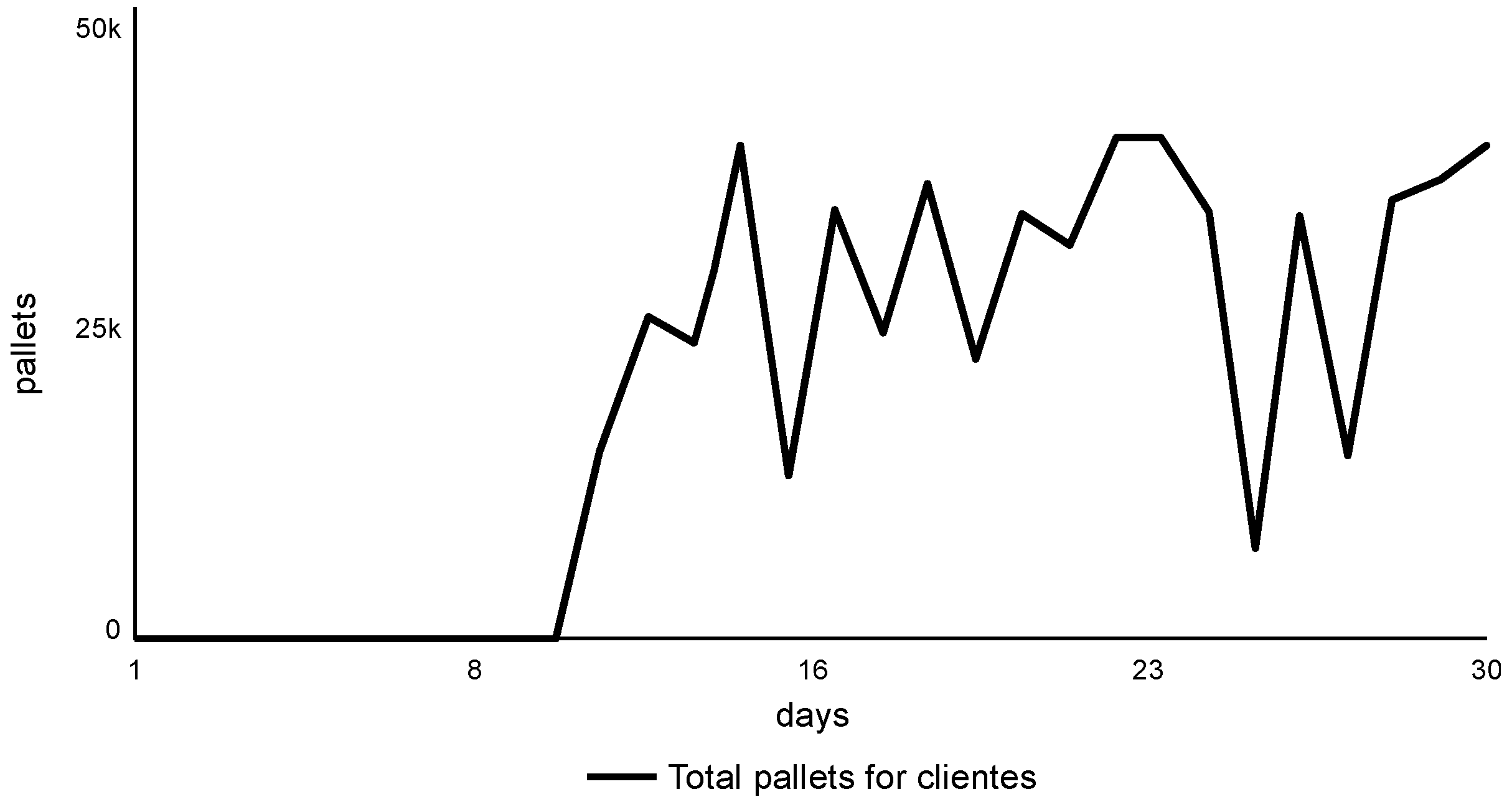
The model simulation was based on Euler’s method developed by Chapra and Canale [8], with the support of Stella® Architect software 3.3. The results of the model are shown in Figure 4, to observe the number of pallets generated at the end of the month.
As observed, the simulation showed that, at the end of the month, 39,493 pallets were made to be delivered to the main client. The relative error validation applied was the first test, as proposed by Barlas [25]; it established that a model was valid if the error rate was lower than 5%; thus, the following Equation (11) was performed:
%   relative   error = Simulated   data Real   data Real   data × 100
The validation test was performed considering the real data provided by the manufacturing company of the average production, which was 38,130 pallets/month.
%   relative   error = 39,493 38,130 39,493 × 100 = 3.4512 %
Therefore, 3.4512 < 5% concluded that the model was valid.
From this result, it could be established that the model came very close to reality; thus, it was valid and reliable given that the relative error was lower than 5%. Therefore, the relative error rate of 3.4512% < 5% was allowed. To confirm the result of the relative error validation test, the following were also applied.
The second test was the extreme conditions proposed by Sterman [19]. This model assigned zero value in the output rate parameter; from there, the production input and output flows were not performed. Additionally, the rest of the structures (stocks, ovens, and conveyors in some cases) were maintained with the initial values; in others they had zero values. See Appendix D.
The third test was the expert validation. This test was presented to the businessmen of the organization, who executed the model and agreed that the results were approximate to reality (also confirmed by the relative error test applied in the first case).
The fourth test was consistent in the units used in the model, where 100% of them were coherent on the left and right sides of each of the developed equations or, in its case, the value of the assigned parameter.

3.5. Building the Graphical Interface with the User

Building the graphical interface with the user represented the technological solution that integrated the previous stages. Starting from the flow and level model and its equations, the graphical interface user was built from the logical behavior of the pallet supply chain dynamics model using Stella® Architect software elements for its design.
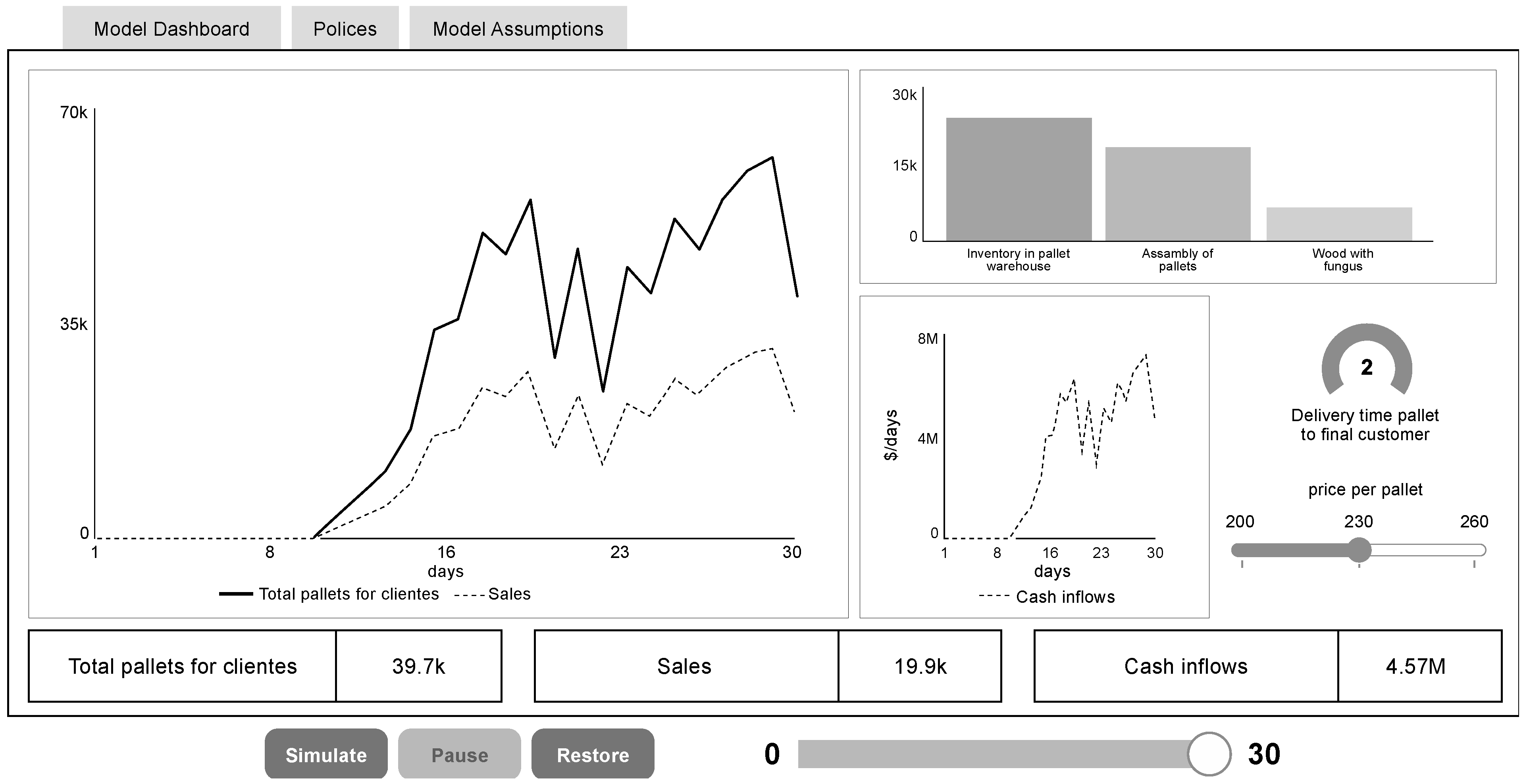
Figure 5 shows one of the screens that composed the graphical interface where different variables were evaluated by using parameters according to the organization policies.
This screen shows six variables that were simulated for decision making based on data. As can be observed, the total pallets to be delivered to the final clients (mostly to the mega beer producer company) showed a daily behavior. The delivery programmed in this simulation at the end of the month was 39,700 pallets compared with 38,200 in real pallet manufacturing company. In this case and according to this situation, the users had the option to consider two policies: (1) pallet time delivery that was between one and two days and (2) sale price for each pallet.
With these data, the graphical behavior can be observed in sales, total pallets for the clients, as well as pallets in the warehouse inventories, the amount of work in assembling, and wood that arrives with fungi. One of the highly relevant datum was the income for the organization at the end of the month.

3.6. Evaluating Scenarios: Normal, Optimistic, and Pessimistic Using Multicriteria Decision Making

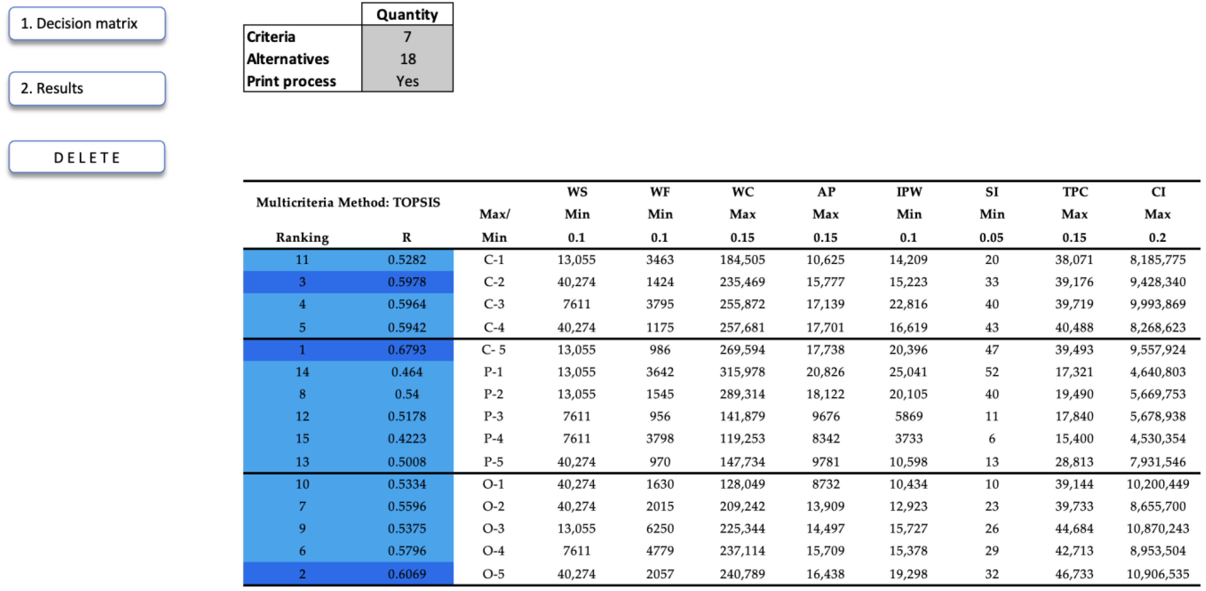
The current value of the pallet supply chain allowed generating five scenarios that were stimulated using the software Stella® Architect (2023 Version 3.3, Isee Systems Inc., Lebanon, NH, USA), as shown in Table 2. Each of the scenarios had eight variables for model analysis. In addition, Table 3 shows the optimization elements used associated with a percentage weighting that was decided by the MCMC methods (based on the overall values) which of the scenarios were the best among the 15 evaluated. Appendix B and Appendix C show the macros represented in the matrixes that allowed obtaining the ranks of the scenarios analyzed by the FUCA and TOPSIS methods.
Considering the TOPSIS and FUCA analyses, the best scenario was number 5, which offered 0.7651, and the worst scenario was number 1.
The MCDM FUCA method is presented in Table 4, showing the lowest value associated with the scenarios to consider as the best positioned.
The best-positioned current scenario was number 5 and the worst was number 1, considering that the values were 1.90 and 4.20, respectively.
The simulation of the 15 scenarios (5 current, 5 pessimistic, and 5 optimistic) was analyzed and compared with TOPSIS and FUCA (see Table 5).
Table 5 shows the comparison of each of the 15 scenarios analyzed, from which the best results were obtained. From the scenario type, the following were determined:
  • Optimistic scenario. The overall value obtained with TOPSIS was 0.6069, given in optimistic scenario 5 and classified in range 2.
  • Pessimistic scenario. The value generated with TOPSIS was 0.5400 for pessimistic scenario 2, classified in rank 8.
  • Current scenario. The value generated with TOPSIS was 0.6793 for current scenario 5, ranked 1.
On the other hand, Table 6 shows the MCDM FUCA method for analyzing the 15 scenarios.
Table 6 shows the three best results obtained from the 15 scenarios and their comparisons, taking into account the following:
  • Optimistic scenario: the overall value with FUCA was 5.5, given in optimistic scenario 5 and classified in rank 2.
  • Pessimistic scenario: the value generated with FUCA was 7.50 for pessimistic scenario 2, ranked 8.
  • Current scenario: the value generated with the FUCA was 5.65 for the current scenario 5, classified in rank 1.
It is important to note that the best scenario in both methods was the current scenario 5 classified in rank 1, with the overall value of 0.6793 for TOPSIS and a value of 5.15 for FUCA.
Table 7 shows the similarity of the FUCA and TOPSIS results in the five optimistic scenarios of the pallet supply chain analyzed.
The scenario with the greatest agreement in both methods was the optimistic 5, where TOPSIS offered 0.6069 as the general value, with ranking in second place. Likewise, FUCA offered 5.5 as the general value and was also classified in second place. Thus, optimistic 5 was the best scenario according to both MCDM methods, taking into account the variable and parameter analyses selected in the dynamic model.

4. Discussion

Developing DS models using scenario simulation and analyses evaluated complex systems in a determined time horizon. The decisions for the interested parties should be highly relevant, considering sustainability as the focus of decisions. In this sense, developing these proposals for the pallet manufacturing company generated quantitative information (social, economic, and environmental data) that has been processed in different scenarios and placed in a graphical interface to facilitate parameter input and modification. Thus, the policies under which the organization would be operating within a determined time were considered.
Discussions of results stem from other empirical studies where most of the DS methodology stages have been implemented.
The merit of the DS model consisted of forming efficient complex feedback mechanisms integrating parameter changes from small to large that were by chance (fortuitous) or continuous. The variation produced when the control variables did not depend linearly on others emerged in the feedback mechanism due to the presence of non-linear relationships [35]. In the same manner, Franco [36] mentioned that no official markers, methods, or tools were available to support and measure enterprise transition from a linear to another circular system.
Using the tools employed in a development project proposal where process flow diagrams were used, Navarro et al. [37] set up models to develop an operational concept of an Internet of Things (IoT) in the palletized distribution supply chain and generated two contributions: (1) the first concept of operations that described how the proposed IoT system was useful and boosted efficiency improvements in the process of designing packing; (2) the second one was the definition of the requirements, using semantics for expanded sequence diagrams and the signal elements of the System Modeling Language (SysML) in the True Model-Based Requirements (TMBR) approach.
Likewise, Ren et al. [38] used simulators for decision making, as the one used in this project, with Stella® Architect, version 3.3, Isee Systems Inc., Lebanon, NH, USA. In their proposal, the authors showed that their work dealt mainly with how to help pallet managers select a specific type of pallet from the cost perspective of the supply chain. AnyLogic version 8.3, The Anylogic Company, Oakbrook Terrace, IL, USA was used to simulate the functioning of the pallet management systems.
On the other hand, Balakirsky [39] utilized USARSim®, version UT3VB1.5, SourceForge Company, San Diego, CA, USA, to explore the role of the simulation to compare to what point the automation metrics could calibrate the quality of a pallet; the simulator allowed studying the interconnection between hidden internal boxes and parameters that could not be determined by mere statistics. Likewise, Guan et al. [40] used simulation to evaluate the shipment of assembly line components in a digital factory based on the process analysis of the pallet dynamic demands.
In the pallet company simulation model, Stella® Architect was used to simulate the scenarios and, from there, selection was made with the multicriteria analysis. The simulators found in [41] concerned the economic analysis of the promising wood products in the forest sector of Letonia. The objective was to analyze three products: bio-oil, lyocell, and xylene. Currently, none of the products are made in Letonia. The system dynamics model was used with the Powersim Studio 8 software to determine which of the products had greater added value and which was more feasible for use.
The use of the model validation techniques to measure the reliability of the proposed model was based on the works of Barlas and Carpenter [10]. These authors established that, since the model was assumed from a real system, it could be false or true. When the adequate algorithms were used and compared with the empirical study, its validity was automatically revealed as false or true. Thus, the result depended on the formal precision of the assumed model. Similarly, Barlas [25] mentioned that, for the model behavior validity, the general validation of the simulation was an important part. The challenge consisted of designing novel quantitative tests appropriate for evaluating the behavior of system dynamics given by the behavior of the composition patterns instead of the individual data points. One of the proposals to validate the model was the test of the relative error.
In this sense, for the pallet project, the relative error test allowed including the results from the real data and assuming the proposed model. The results obtained allowed assuming that the model was close to reality starting from the compliance of the criterium established, considering the result of the simulation data.
The use of the methods that considered the analysis of the most relevant ones were important in developing the model scenarios. For this purpose, FUCA and TOPSIS multicriteria analyses were used, as in the works of Duc [42], who demonstrated that the FUCA method could be used in mechanical processing for multicriteria decision making that did not require data standardization. To select the best scenarios from the simulation and sensitivity analysis, eight decision variables were considered, which competed based on the maximum and minimum optimization criteria according to Bachar et al. [26]. These authors used a traditional technique to examine the global optimization of the profit and decision function variables in an energy consumption project of an intelligent manufacturing company, where the demand was considered flexible. In the same manner, in another study in demand analysis, Raj et al. [27] developed a sustainable ecological production model taking into account the variable demand. These authors found that controlling the fluctuating demand and rebuilding imperfect products made the model production profitable. Soumya et al. [28] demonstrated the application of the proposed solution through numerical and graphical sensitivity analyses.
In the same manner, Baydaş and Pamucar [43] applied seven multicriteria methods to evaluate the performance of companies in the financial sector, demonstrating that FUCA was the most simple methodology compared with the others they used (PROMETHEE, FUCA, TOPSIS, SAW, CODAS, COPRAS, and MOORA). On the other hand, Narendra et al. [44] developed a model applying system dynamics to describe the wood biomass production potential starting from rehabilitating degraded lands. The result showed that all scenarios achieved reducing the degraded land area by 16%. The energetic wood plantations could reduce the numbers of unemployment by one half of the simulated amount while applying a moderate, optimistic, or very optimist scenario; the number of unemployment would only remain one quarter by 2040. The optimistic scenario was considered applied in the degraded land rehabilitation.
Finally, the graphical user interface (GUI)-supported software was usually large and complex and difficult to implement, debug, and modify, as established by Myers [45]. This software generated the communication between decision makers and the technological solution (GUI), allowing the use of graphical elements, as well as a table of data that allowed having the information in the time line established according to the policies and rules of the organization. It is important to highlight that, for the organization under study, GUI was supported by mathematical models that generated each of the variable behaviors starting from the defined parameters according to the interest of the organization.
This solution considered elements of sustainability, where SD was used as an analysis tool [46,47,48] and scenario analysis was used for data-driven decision making [49,50,51]. The benefits for the company and decision makers had theoretical and methodological contributions as a basis. From the theoretical perspective, different authors’ contributions were used, using the system dynamics approach based on optimization with diverse mathematical algorithms to manage inventories from products made and delivered [52].

5. Conclusions

The use of DS in the projects related with the supply chain projects allowed evaluating the methodology potential in the organization environment dedicated to the pallet production conditioned to the important demands for mega companies of the Southern Sonora region. This analysis allowed the pallet manufacturing company to have and include critical elements in providing wood inputs, pallet production, and the distribution process in compliance with the quality and time demanded.
The most relevant conclusions in the present research study were having the support of a system dynamics model for decision making concentrated in the graphical user interface, which made it more accessible to the persons working, without necessarily having knowledge of the system. The model considered 31 variables and 8 parameters that were included in the different equations.
On the other hand, developing the scenarios helped the company to observe a time line of the production and inventory behavior. In this manner, they could satisfy the demands of the main client and make the necessary preparations to comply with each one of the (max/mini) criteria of the eight variables of major relevance associated with the model.
Likewise, the support of the proposed procedure was based on the real and theoretical empirical studies that provided assurance to future decisions, such as the scenario with the greatest agreement in both methods, e.g., the optimistic 5 where TOPSIS offered 0.6069 as the general value, with ranking in second place And, in the same manner, where FUCA offered 5.5. as the general value, with ranking in second place.
The previous data were provided by the company for model construction. Thus, by applying the test of the relative error percentage and comparing it with reality, the result had 3.4% of relative error against the 5% allowed, which supposed that the model adhered to reality.
On the other hand, the academic environment allowed promoting real cases for students and academics to include as part of the curriculum courses in teaching system dynamics methodology.
Future work to be performed should include variables that allow evaluating alternatives of a more robust circular economy in the dynamic model to take advantage of the rejected pallet and wood waste, which in time generates huge inventories that may be revalued to generate income for the organization.

Author Contributions

Conceptualization, E.A.L.-L. and A.B.-S.; methodology, E.A.L.-L.; software, E.A.L.-L.; validation, M.P.G.A.-Q., J.P.-V. and A.A.N.-F.; formal analyses, E.A.L.-L. and A.B.-S.; investigation, E.A.L.-L.; A.B.-S.; M.P.G.A.-Q., J.P.-V. and A.A.N.-F.; resources, E.A.L.-L.; data curation, E.A.L.-L.; writing—original draft preparation, E.A.L.-L.; writing—review and editing, E.A.L.-L. and A.B.-S.; visualization, A.B.-S.; supervision, A.B.-S.; project administration, E.A.L.-L.; funding acquisition, E.A.L.-L. All authors have read and agreed to the published version of the manuscript.

Funding

This research received no external funding.

Institutional Review Board Statement

Not applicable.

Informed Consent Statement

Not applicable.

Data Availability Statement

Not applicable.

Acknowledgments

All authors are grateful to Instituto Tecnológico de Sonora for the support through the project PROFAPI_2023_CA_015; to CONAHCYT (Consejo Nacional de Humanidades, Ciencia y Tecnología) for the support to ITSON National Laboratory for Transportation Systems and Logistics; to Diana Fischer for translation edition.

Conflicts of Interest

The authors declare no conflict of interest.

Appendix A. Equations, Properties, and Units

EquationPropertiesUnits
Assembly_of_pallets(t)=Assembly_of_pallets (t-dt) + (“Entry-assembly_flow_of_pallets”- towards_sealing- Waste) × dtINIT Assembly_of_pallets = 0pallet
Conveyor_to_distrubution_of_pallets(t)=Conveyor_to_distrubution_of_pallets (t-dt) + (Final_brushing -loading_of_pallets_on_trucks) × dtINIT Conveyor_to_distrubution_of_pallets = 0
TRANSIT TIME = 1
CAPACITY = 30,000
CONTINUOUS
ACCEPT MULTIPLE BATCHES
pallet
Conveyor_to_storage_of_pallets(t) = Conveyor_to_storage_of_pallets (t-dt) + (output_1_to_storage_of_pallets + output_2_yo_storage_of_pallets-Warehousing_of_Finished_product) × dtINIT Conveyor_to_storage_of_pallets = 1
TRANSIT TIME = 0.03
CONTINUOUS
ACCEPT MULTIPLE BATCHES
pallet
Inventory_in_pallet_warehouse(t) = Inventory_in_pallet_warehouse (t-dt) + (Warehousing_of_Finished_product-Final_brushing) × dtINIT Inventory_in_pallet_warehouse = 0pallet
Inventory_in_transit(t) = inventory_in_transit (t - dt) + (pallets_in_trucks - final_client) × dtINIT inventory_in_transit = STEP(1,RANDOM (3100, 3200))
COOK TIME = 1
CAPACITY = 3200
FILL TIME = 0.3
ACCEPT SINGLE
BATCHSPLIT BATCHES
pallet
Loading_trucks(t) = Loading_trucks (t - dt) + (loading_of_pallets_on_trucks - pallets_in_trucks) × dtINIT Loading_trucks = 0pallet
Oven_1(t) = Oven_1(t-dt) + (Output_to_oven_1-output_1_to_storage_of_pallets) × dtINIT Oven_1 = 0
COOK TIME = 1
CAPACITY = 10,000
FILL TIME = 0.03
ACCEPT SINGLE
BATCHSPLIT BATCHES
pallet
Oven_2(t) = Oven_2(t-dt) + (Output_to_oven_2-output_2_yo_storage_of_pallets) × dtINIT Oven_2 = 0
COOK TIME = 1
CAPACITY = 30,000
FILL TIME = 0.03
ACCEPT SINGLE
BATCHSPLIT BATCHES
pallet
Queue_1(t) = Queue_1(t-dt) + (arrival_at_sealing_pallets-Output_to_oven_1-Output_to_oven_2) × dtINIT Queue_1 = 0pallet
Sawdust_Inventory(t) = Sawdust_Inventory(t-dt) + (Sawdust) × dtINIT Sawdust_Inventory = 0ton sawdust
Total_pallets_for_clients(t) = Total_pallets_for_clients(t-dt) + (final_client-Sales) × dtINIT Total_pallets_for_clients = 0pallet
Transfer_to_sealing(t) = transfer_to_sealing (t-dt) + (towards_sealing-arrival_at_sealing_pallets) × dtINIT transfer_to_sealing = 0
TRANSIT TIME = 1
CAPACITY = 30,000
CONTINUOUS
ACCEPT MULTIPLE BATCHES
pallet
Washing_in_chlorine(t) = Washing_in_chlorine (t-dt) + (output_of_wood_lots-chlorination) × dtINIT Washing_in_chlorine = 0
COOK TIME = 0.3
CAPACITY = 3200
FILL TIME = 0.1
ACCEPT SINGLE
BATCHSPLIT BATCHES
ft-wood
Wood_brushing(t) = Wood_brushing (t-dt) + (cleaning - brushing) × dtINIT Wood_brushing = 0
TRANSIT TIME = 1
CAPACITY = 3000
CONTINUOUS
ACCEPT MULTIPLE BATCHES
ft-wood
Wood_Clean(t) = Wood_Clean (t-dt) + (Incoming_flow_of_clean_wood) × dtINIT Wood_Clean = 0ft-wood
Wood_lots(t) = wood_lots (t-dt) + (brushing-oupu_of_wood_lots) × dtINIT wood_lots = 0ft-wood
Wood_storage(t) = Wood_storage(t-dt) + (Wooden_wood-Output_to_production) × dtINIT Wood_storage = 0ft-wood
Woods_with_fungus(t) = Woods_with_fungus (t-dt) + (“FE-Wood_with_fungus”-cleaning) × dtINIT Woods_with_fungus = 0ft-wood
arrival_at_sealing_pallets = CONVEYOR OUTFLOWATTRIBUTE VALUE = time_of_arrival_sealedpallet/day
Brushing = CONVEYOR OUTFLOWATTRIBUTE VALUE = arrival_timeft-wood/day
Chlorination = OVEN OUTFLOWNoneft-wood/day
Cleaning = Woods_with_fungus x ”%_of_wood”Noneft-wood/day
“Entry-assembly_flow_of_pallets” = Wood_Clean/ft_of_wood_per_palletNonepallet/day
“FE-Wood_with_fungus” = Output_to_production × ”%_wood_with_fungus”Noneft-wood/day
Final_brushing = Inventory_in_pallet_warehouse/rate_of_wood_brushedNonepallet/day
final_client = OVEN OUTFLOWNonepallet/day
Incoming_flow_of_clean_wood = “%_clean_wood” × (Output_to_production + chlorination)Noneft-wood/day
loading_of_pallets_on_trucks = CONVEYOR OUTFLOWATTRIBUTE VALUE = Truck_loading_timepallet/day
output_of_wood_lots = QUEUE OUTFLOWNoneft-wood/day
output_1_to_storage_of_pallets = OVEN OUTFLOWINFLOW PRIORITY: 1pallet/day
output_2_yo_storage_of_pallets = OVEN OUTFLOWINFLOW PRIORITY: 2pallet/day
Output_to_oven_1 = QUEUE OUTFLOWOUTFLOW PRIORITY: 1pallet/day
Output_to_oven_2 = QUEUE OUTFLOWOUTFLOW PRIORITY: 2pallet/day
Output_to_production = Wood_storage x Output_rateNoneft-wood/day
pallets_in_trucks = QUEUE OUTFLOWNonepallet/day
Sales = Total_pallets_for_clients/Delivery_time_palletsNonepallet/day
Sawdust = Waste x Convertion_rateNoneton sawdust/day
towards_sealing = Assembly_of_pallets/sealing_timeOUTFLOW PRIORITY: 1pallet/day
Warehousing_of_Finished_product = CONVEYOR OUTFLOWNonepallet/day
Waste = Assembly_of_pallets x Waste_rateOUTFLOW PRIORITY: 2pallet/day
Wooden_wood = IF Diference < 38,752 THEN Orders_amount/Delivery_time ELSE keep_minimum_inventoriesNoneft-wood/day
“%_clean_wood” = RANDOM (0.21, 1)Nonedmnl
“%_of_wood” = RANDOM (0.7, 0.8)None1/day
“%_wood_with_fungus” = RANDOM (0.02, 0.2)Nonedmnl
arrival_time = POISSON(1,0.4555, 1, 3200)None1/day
cash_inflows = Sales*Sales_price_per_palletNoneUSD/day
Convertion_rate = 0.001Noneton steelrin/pallet
Delivery_time = 2Noneday
Delivery_time_pallets = RANDOM (1, 2)Noneday
Difference = Storage_capacity-Wood_storageNoneft-wood
ft_of_wood_per_pallet = 12.11Noneft-wood/pallet*day
keep_minimum_inventories = 38,752Noneft-wood/day
Orders_amount = 10,000Noneft-wood
Output_rate = 0.8None1/day
rate_of_wood_brushed = RANDOM (1, 2)Noneday
Sales_price_per_pallet = 260NoneUSD/pallet
sealing_time = 1Noneday
Storage_capacity = 38,752Noneft-wood
time_of_arrival_sealed = POISSON(1, 0.4555, 1, 3200)None1/day
Truck_loading_time = POISSON(1, 0.4555, 1, 3200)Noneday
Waste_rate = 0.2None1/day

Appendix B. Macros Used to Determine TOPSIS Ranking
Sustainability 15 11766 i001

Appendix C. Macros Used to Determine FUCA Ranking

Sustainability 15 11766 i002

Appendix D. Model Tested under Extreme Conditions Using the Order Rate = 0
Sustainability 15 11766 i003

References

  1. Pedroso, C.B.; Tate, W.L.; da Silva, A.L.; Carpinetti, L.C.R. Supplier development adoption: A conceptual model for triple bottom line (TBL) outcomes. J. Clean. Prod. 2021, 314, 127886. [Google Scholar] [CrossRef]
  2. Silver, E.A.; Pyke, D.F.; Peterson, R. Inventory Management and Production Planning and Scheduling, 3rd ed.; Wiley: Chichester, UK, 1998. [Google Scholar]
  3. Forrester, J. Dinámica Industrial, 2nd ed.; El Ateneo: Buenos Aires, Argentina, 1981. [Google Scholar]
  4. Senge, P. La Quinta Disciplina, 2nd ed.; Granica: Buenos Aires, Argentina, 2005. [Google Scholar]
  5. Aracil, J.; Gordillo, F. Dinámica de Sistemas; Alianza: Madrid, Spain, 1997. [Google Scholar]
  6. Richardson, G.; Pugh, A., III. Introduction to System Dynamics Modeling with Dynamo. J. Oper. Res. Soc. 1997, 48, 1146. [Google Scholar] [CrossRef]
  7. Richmond, B. Introduction to System Thinking, STELLA®; Isse Systems: Lebanon, NH, USA, 2013; ISBN 100970492111. Available online: https://iseesystems.com/store/books/intro-systems-thinking/ (accessed on 20 April 2023).
  8. Chapra, S.; Canale, R. Numerical Methods for Engineers, 7th ed.; Mc Graw Hill Education: New York, NY, USA, 2015. [Google Scholar]
  9. Kleijnen, J. Verification and validation of simulation models. Eur. J. Oper. Res. 1995, 82, 145–162. [Google Scholar] [CrossRef] [Green Version]
  10. Barlas, Y.; Carpenter, S. Philosophical roots of model validation: Two paradigms. Syst. Dyn. Rev. 1990, 6, 148–166. [Google Scholar] [CrossRef]
  11. Schwartz, P. The Art of the Long View: “Planning for the Future in an Uncertain World”; Currency Doubleday: New York, NY, USA, 1996. [Google Scholar]
  12. Fernando, M.M.L.; Escobedo, J.L.P.; Azzaro-Pantel, C.; Pibouleau, L.; Domenech, S.; Aguilar-Lasserre, A. Selecting the best portfolio alternative from a hybrid multi objective GA-MCDM approach for New Product Development in the pharmaceutical industry. In Proceedings of the IEEE Symposium on Computational Intelligence in Multicriteria Decision-Making (MDCM), Paris, France, 11–15 April 2011; pp. 159–166. [Google Scholar]
  13. Wang, Z.; Rangaiah, G.P. Application and Analysis of Methods for Selecting an Optimal Solution from the Pareto-Optimal Front obtained by Multi-objective Optimization. Ind. Eng. Chem. Res. 2016, 56, 560–574. [Google Scholar] [CrossRef]
  14. Saha, S.; Sarkar, B.; Sarkar, M. Application of improved meta heuristic algorithms for green preservation technology management to optimize dynamical investments and replenishment strategies. Math. Comput. I Simul. 2023, 209, 426–450. [Google Scholar] [CrossRef]
  15. Lagarda-Leyva, E.A.; Ruiz, A. A Systems Thinking Model to Support Long-Term Bearability of the Healthcare System: The Case of the Province of Quebec. Sustainability 2019, 11, 7028. [Google Scholar] [CrossRef] [Green Version]
  16. Oulasvirta, A.; Dayama, N.R.; Shiripour, M.; John, M.; Karrenbauer, A. Combinatorial Optimization of Graphical User Interface Designs. Proc. IEEE 2020, 108, 434–464. [Google Scholar] [CrossRef]
  17. Lagarda-Leyva, E.; y Zavala, C. Plan Estratégico 2021–2026 Para la Asociación de Productores del Valle del Mayo, Navojoa, México. 2021. Available online: https://docs.google.com/presentation/d/13cjvOsP0UjP561Nv0d3tf4gqpsKgm2sn06mSSvO0uFk/edit?usp=sharing (accessed on 4 April 2023).
  18. Forrester, J.W. System dynamics, systems thinking, and soft OR. Syst. Dyn. Rev. 1994, 10, 245–256. [Google Scholar] [CrossRef]
  19. Sterman, J. Business Dynamics: Systems Thinking and Modeling for a Complex World; McGraw Hill: New York, NY, USA, 2000. [Google Scholar]
  20. Bueno-Solano, A.; Cedillo-Campos, M.G. Dynamic Impact on Global Supply Chains Performance of Disruptions Propagation Produced by Terrorist Acts. Transp. Res. Part E Logist. Transp. Rev. 2014, 61, 1–12. [Google Scholar] [CrossRef]
  21. Gnoni, M.; Lettera, G.; Rollo, A. A simulation comparison analysis of effective pallet management scenarios. In Proceedings of the IEEE International Conference on Industrial Engineering and Engineering Management, Singapore, 6–9 December 2011; pp. 1228–1232. [Google Scholar] [CrossRef]
  22. Elia, V.; Gnoni, M.G. Designing an effective closed loop system for pallet management. Int. J. Prod. Econ. 2015, 170, 730–740. [Google Scholar] [CrossRef]
  23. Newman, W.E.; Boe, W.J.; Denzler, D.R. Examining the use of dedicated and general purpose pallets in a dedicated flexible manufacturing system. Int. J. Prod. Res. 1991, 29, 2117–2133. [Google Scholar] [CrossRef]
  24. Mikati, N. Dependence of lead time on batch size studied by a system dynamics model. Int. J. Prod. Res. 2010, 48, 5523–5532. [Google Scholar] [CrossRef]
  25. Barlas, Y. Multiple tests for validation of system dynamics type of simulation models. Eur. J. Oper. Res. 1989, 42, 59–87. [Google Scholar] [CrossRef]
  26. Bachar, R.K.; Bhuniya, S.; Ghosh, S.K.; Sarkar, B. Controllable Energy Consumption in a Sustainable Smart Manufacturing Model Considering Superior Service, Flexible Demand, and Partial Outsourcing. Mathematics 2022, 10, 4517. [Google Scholar] [CrossRef]
  27. Bachar, R.K.; Bhuniya, S.; Ghosh, S.K.; Sarkar, B. Sustainable green production model considering variable demand, partial outsourcing, and rework. AIMS Environ. Sci. 2022, 9, 325–353. [Google Scholar] [CrossRef]
  28. Hota, S.K.; Ghosh, S.K.; Sarkar, B. A solution to the transportation hazard problem in a supply chain with an unreliable manufacturer. AIMS Environ. Sci. 2022, 9, 354–380. [Google Scholar] [CrossRef]
  29. Lagarda-Leyva, E.A.; Bueno-Solano, A.; Morales-Mendoza, L.F. System Dynamics and Graphical Interface Modeling of a Fig-Derived Micro-Producer Factory. Sustainability 2022, 14, 13043. [Google Scholar] [CrossRef]
  30. Baydaş, M.; Elma, O.E.; Pamučar, D. Exploring the specific capacity of different multi criteria decision making approaches under uncertainty using data from financial markets. Expert Syst. Appl. 2022, 197, 116755. [Google Scholar] [CrossRef]
  31. Truong, N.X.; Thinh, H.X. Combined PIPRECIA method and modified FUCA method for selection of lathe. J. Appl. Eng. Sci. 2022, 20, 1355–1365. [Google Scholar] [CrossRef]
  32. Son, N.H.; Hieu, T.T.; Thang, N.M.; Tan, H.N.; Can, N.T.; Thao, P.T.; Bao, N.C. Choosing the best machine tool in mechanical manufacturing. EUREKA Phys. Eng. 2023, 2, 97–109. [Google Scholar] [CrossRef]
  33. Luna, R.; López, F.; Pérez-Correa, J.R. Design of optimal wine distillation recipes using multi-criteria decision-making techniques. Comput. Chem. Eng. 2021, 145, 107194. [Google Scholar] [CrossRef]
  34. Ouattara, A.; Pibouleau, L.; Azzaro-Pantel, C.; Domenech, S.; Baudet, P.; Yao, B. Economic and environmental strategies for process design. Comput. Chem. Eng. 2012, 36, 174–188. [Google Scholar] [CrossRef] [Green Version]
  35. Mak, T.M.; Wang, L.; Tsang, D.C. System dynamics on wood and yard waste management. In Waste Biorefinery; Elsevier: Amsterdam, The Netherlands, 2020; pp. 559–578. [Google Scholar]
  36. Franco, M.A. A system dynamics approach to product design and business model strategies for the circular economy. J. Clean. Prod. 2019, 241, 118327. [Google Scholar] [CrossRef]
  37. Navarro, N.; Horvath, L.; Salado, A. Design of an IoT System for the Palletized Distribution Supply Chain with Model-Based Systems Engineering Tools. Systems 2022, 10, 4. [Google Scholar] [CrossRef]
  38. Ren, J.; Zhao, Q.; Liu, B.; Chen, C. Selection of pallet management strategies from the perspective of supply chain cost with Anylogic software. PLoS ONE 2019, 14, e0217995. [Google Scholar] [CrossRef]
  39. Balakirsky, S.; Proctor, F.; Kramer, T.; Kolhe, P.; Christensen, H.I. Using Simulation to Assess the Effectiveness of Pallet Stacking Methods. In Simulation, Modeling, and Programming for Autonomous Robots. SIMPAR 2010. Lecture Notes in Computer Science; Ando, N., Balakirsky, S., Hemker, T., Reggiani, M., von Stryk, O., Eds.; Springer: Berlin/Heidelberg, Germany, 2010; Volume 6472. [Google Scholar] [CrossRef]
  40. Guan, Z.; Cao, L.; Wang, C.; Cui, Y.; Shao, X. Simulation of Logistics System with Aspect of Pallet Requirements Optimization Based on Digital Factory. In Advances in Automation and Robotics, Lecture Notes in Electrical Engineering; Lee, G., Ed.; Springer: Berlin/Heidelberg, Germany, 2011; Volume 1. [Google Scholar] [CrossRef]
  41. Gravelsins, A.; Blumberga, A.; Blumberga, D.; Muizniece, I. Economic analysis of wood products: System dynamics approach. Energy Procedia 2017, 128, 431–436. [Google Scholar] [CrossRef]
  42. Duc, T. Application of fuca method for multi-criteria decision making in mechanical machining processes. Oper. Res. Eng. Sci. Theory Appl. 2022, 5, 131–152. [Google Scholar] [CrossRef]
  43. Baydas, M.; Pamučar, D. Determining Objective Characteristics of MCDM Methods under Uncertainty: An Exploration Study with Financial Data. Mathematics 2022, 10, 1115. [Google Scholar] [CrossRef]
  44. Narendra, B.H.; Widiatmaka, W.; Kusmana, C.; Karlinasari, L.; Machfud, M. A System Dynamics Model for Wood-Based Renewable Energy Production from Degraded Land Rehabilitation. Pol. J. Environ. Stud. 2021, 30, 5643–5656. [Google Scholar] [CrossRef]
  45. Myers, B. Challenges of HCI Design and Implementation. ACM Interact. 1994, 1, 73–83. [Google Scholar] [CrossRef]
  46. Shamsuddoha, M.; Nasir, T.; Hossain, N.U.I. A Sustainable Supply Chain Framework for Dairy Farming Operations: A System Dynamics Approach. Sustainability 2023, 15, 8417. [Google Scholar] [CrossRef]
  47. Shi, Q.; Li, Z.; Xu, Y.; Yan, T.; Chen, M. Dynamic Scenario Simulations of Sustainable Rural and Towns Development in China: The Case of Wujiang District. Sustainability 2023, 15, 8200. [Google Scholar] [CrossRef]
  48. Bardi, U. Mind Sized World Models. Sustainability 2013, 5, 896–911. [Google Scholar] [CrossRef] [Green Version]
  49. Walker, W.E.; Haasnoot, M.; Kwakkel, J.H. Adapt or Perish: A Review of Planning Approaches for Adaptation under Deep Uncertainty. Sustainability 2013, 5, 955–979. [Google Scholar] [CrossRef] [Green Version]
  50. Kwakkel, J.H.; Auping, W.; Pruyt, E. Dynamic scenario discovery under deep uncertainty: The future of copper. Technol. Forecast. Soc. Change 2012, 80, 789–800. [Google Scholar] [CrossRef]
  51. Lempert, R.J.; Bryant, B.P.; Bankes, S. Comparing Algorithms for Scenario Discovery; WR-557-NSF; RAND: Santa Monica, CA, USA, 2008. [Google Scholar]
  52. Mukherjee, T.; Sangal, I.; Sarkar, B.; Alkadash, T.M. Mathematical estimation for maximum flow of goods within a cross-dock to reduce inventory. Math. Biosci. Eng. 2022, 19, 13710–13731. [Google Scholar] [CrossRef] [PubMed]
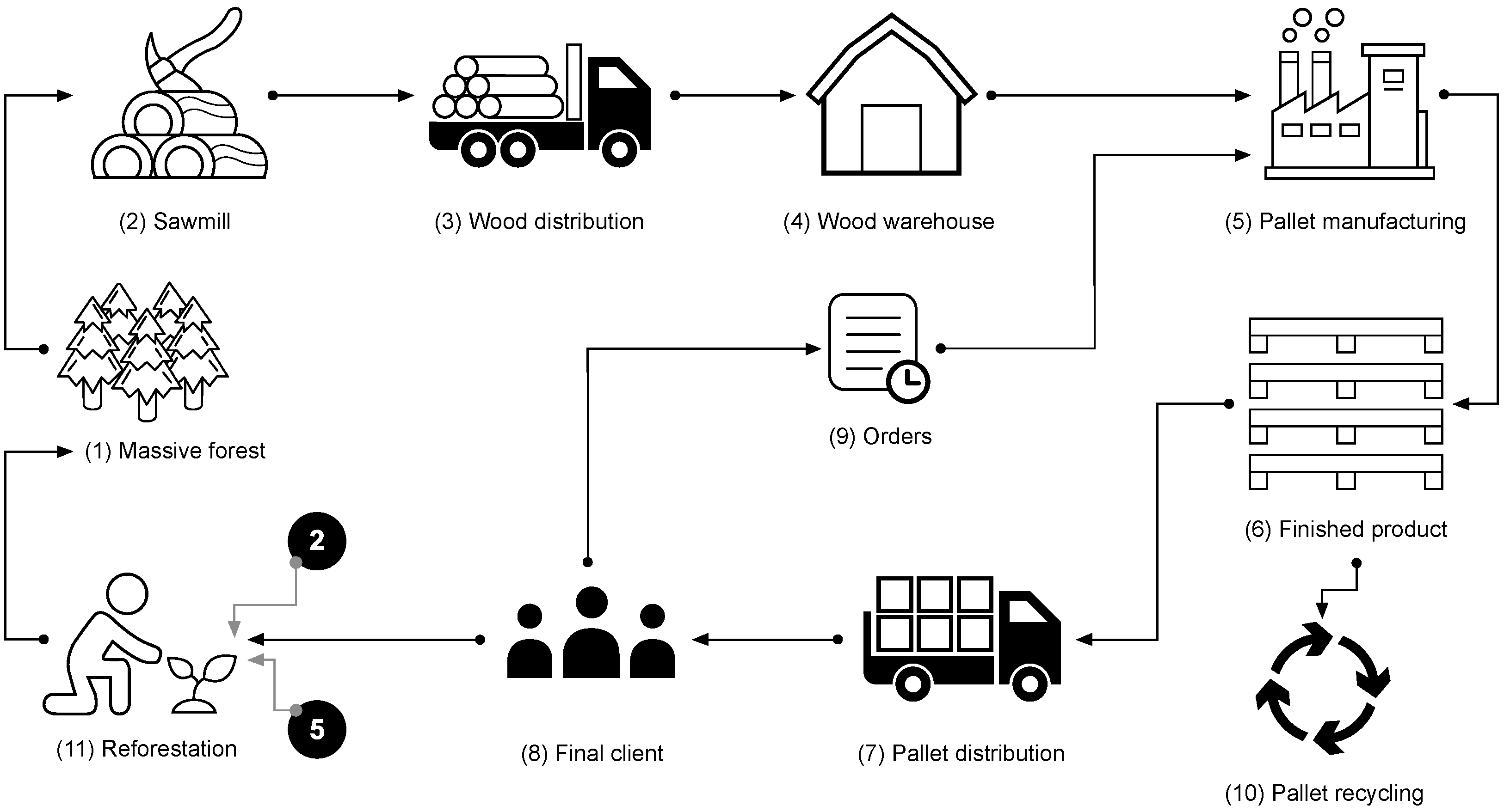
Figure 1. Map of the pallet supply chain. Source: own production (2023).
Sustainability 15 11766 g001
Figure 2. Causal loop diagram for the pallet supply chain. Source: own production (2023).
Sustainability 15 11766 g002
Figure 3. Stock and flow diagram for the pallet factory. Source: own production (2023).
Sustainability 15 11766 g003
Figure 4. Simulation of total pallets for clients. Source: own production (2023).
Sustainability 15 11766 g004
Figure 5. Graphical user interface of model. Source: own production (2023).
Sustainability 15 11766 g005
Table 1. Main contributions from each of the authors.
Author (s)NoveltyStudy Effectiveness
[3]Founder of the dynamics system methodologyApplied methodology of different business environments; the methodology is the basis of the proposed construction for the industrial sector.
[4,6]Use of the systemic thought as support for the causal diagram constructionVariable and parameter complexity analysis from the systemic approach; bases for the selection of variables and their relationship presented in different R and B loops.
[7]Guide for using Stella Architect software version 3.3 Contributions on the use of Stella Architect Software for simulation, sensitivity analysis, design, and development of the graphical user interface.
[8]Set up the logics in which the methods of Euler, Runge Kuta of order 2 and 4 functionUse of the iterative numerical resolution of differential equations (Euler and compared with Runge–Kutta).
[9,10,19,25]Validation methodsOffer different validation methods of system dynamics models.
[11]Study of qualitative scenarios Theoretical basis to understand the exogenous and endogenous variable behavior in qualitative environments.
[12,13]Use of the multicriteria method for the selection of the best scenarios Selection of the most critical variables to apply a multicriteria decision making TOPSIS and FUCA.
[14,26,27,28]Mathematical models and metaheuristic algorithms Using mathematical and metaheuristic models applied in the supply chain and manufacturing under a sustainable approach.
[15]Causal diagram development for the health sector analysisProposal of the causal R and B models to represent the complexity of the hospital system of the Province of Quebec, Canada.
[16]Graphical user interface Design of graphical user interface with combinatorial optimization problems.
[5,18,19,29]Initial contributions of system dynamics methodologyMethodologies with different applications in businesses using validation technique models.Basis of theoretical and practical application in different environments, such as the supply chain analysis projects.
[21,22,23]Empirical support studies to develop causal loops, simulating optimistic/pessimistic scenarios from current ones and their validation in the pallet manufacturing businessDeveloped a simulation model to compare scenarios in terms of time of the provider service and internal and global operation costs.
Designing closed causal loops and use of simulation as supported tools developed to help logistics decisions in organizations under different scenarios.
Table 2. Main contributions for each of the authors.
CriteriaWSWFCI
ObjectiveMax/MinMax/MinMax/Min
WeightWhole Value 0 and 1Value between 0 and 1Whole Value 0 and 1
Alternative 1
Alternative 2
Alternative 15
Source: own production (2023).
Table 3. The MCDM TOPSIS for the analysis of the current five scenarios.
Multicriteria Method: TOPSIS WSWFWCAPIPWSITPCCI
Max/
Min
MinMinMaxMaxMinMinMaxMax
RankingR0.10.10.150.150.10.050.150.2
50.4592C-113,0553463184,50510,62514,2092038,0718,185,775
40.4926C-240,2741424235,46915,77715,2233339,1769,428,340
30.5407C-376113795255,87217,13922,8164039,7199,993,869
20.5109C-440,2741175257,68117,70116,6194340,4888,268,623
10.7651C-513,055986269,59417,73820,3964739,4939,557,924
Notes: WS—wood storage (units); WF—wood with fungus (units); WC—wood clean (units); AP—assembly pallets (units); IPW—inventory in pallet warehouse (units); SI—sawdust inventory (tons); TPC—total pallets for clients (units); CI—cash inflows (MXN); R—relative proximate value; MCDM—multicriteria decision making. Source: own production (2023).
Table 4. FUCA for the analyses of current five scenarios.
Multicriteria Method: FUCA WSWFWCAPIPWSITPCCI
Max/
Min
MinMinMaxMaxMinMinMaxMax
RankingWeight Sum0.10.10.150.150.10.050.150.2
54.20C-113,0553463184,50510,62514,2092038,0718,185,775
43.50C-240,2741424235,46915,77715,2233339,1769,428,340
32.65C-376113795255,87217,13922,8164039,7199,993,869
22.55C-440,2741175257,68117,70116,6194340,4888,268,623
11.90C-513,055986269,59417,73820,3964739,4939,557,924
Notes: WS—wood storage (units); WF—wood with fungus (units); WC—wood clean (units); AP—assembly pallets (units); IPW—inventory in pallet warehouse (units); SI—sawdust inventory (tons); TPC—total pallets for clients (units); CI—cash inflows (MXN); R—relative proximate value. Source: own production (2023).
Table 5. Analysis of scenarios with the MCDM TOPSIS method.
Multicriteria Method: TOPSIS WSWFWCAPIPWSITPCCI
Max/
Min
MinMinMaxMaxMinMinMaxMax
RankingR0.10.10.150.150.10.050.150.2
110.5282C-113,0553463184,50510,62514,2092038,0718,185,775
30.5978C-240,2741424235,46915,77715,2233339,1769,428,340
40.5964C-376113795255,87217,13922,8164039,7199,993,869
50.5942C-440,2741175257,68117,70116,6194340,4888,268,623
10.6793C- 513,055986269,59417,73820,3964739,4939,557,924
140.4640P-113,0553642315,97820,82625,0415217,3214,640,803
80.5400P-213,0551545289,31418,12220,1054019,4905,669,753
120.5178P-37611956141,879967658691117,8405,678,938
150.4223P-476113798119,25383423733615,4004,530,354
130.5008P-540,274970147,734978110,5981328,8137,931,546
100.5334O-140,2741630128,049873210,4341039,14410,200,449
70.5596O-240,2742015209,24213,90912,9232339,7338,655,700
90.5375O-313,0556250225,34414,49715,7272644,68410,870,243
60.5796O-476114779237,11415,70915,3782942,7138,953,504
20.6069O-540,2742057240,78916,43819,2983246,73310,906,535
Note 1: WS—wood storage (units); WF—wood with fungus (units); WC—wood clean (units); AP—assembly pallets (units); IPW—inventory in pallet warehouse (units); SI—sawdust inventory (tons); TPC—total pallets for clients (units); CI—cash inflows (MXN). Note 2: R—relative proximate value; C—current; P—pessimistic; O—optimistic; MCDM—multicriteria decision making. Source: own production (2023).
Table 6. Analysis of scenarios with the MCDM FUCA method.
MCDM Method: FUCA WSWFWCAPIPWSITPCCI
Max
Min
MinMinMaxMaxMinMinMaxMax
RankingGeneral Value0.10.10.150.150.10.050.150.2
139.45C-113,0553463184,50510,62514,2092038,0718,185,775
77.15C-240,2741424235,46915,77715,2233339,1769,428,340
36.10C-376113795255,87217,13922,8164039,7199,993,869
46.15C-440,2741175257,68117,70116,6194340,4888,268,623
15.15C-513,055986269,59417,73820,3964739,4939,557,924
108.35P-113,0553642315,97820,82625,0415217,3214,640,803
87.50P-213,0551545289,31418,12220,1054019,4905,669,753
129.30P-37611956141,879967658691117,8405,678,938
1512.00P-476113798119,25383423733615,4004,530,354
149.65P-540,274970147,734978110,5981328,8137,931,546
118.85O-140,2741630128,049873210,4341039,14410,200,449
98.15O-240,2742015209,24213,90912,9232339,7338,655,700
56.75O-313,0556250225,34414,49715,7272644,68410,870,243
66.80O-476114779237,11415,70915,3782942,7138,953,504
25.50O-540,2742057240,78916,43819,2983246,73310,906,535
Note 1: WS—wood storage (units); WF—wood with fungus (units); WC—wood clean (units); AP—assembly pallets (units); IPW—inventory in pallet warehouse (units); SI—sawdust inventory (tons); TPC—total pallets for clients (units); CI—cash inflows (MXN). Note 2: C—current; P—pessimistic; O—optimistic; MCDM—multicriteria decision making. Source: own production (2023).
Table 7. Comparative MCDM FUCA and TOPSIS method for analyses in optimistic scenarios.
Optimistic ScenariosMCDM1 = TOPSISMCDM2 = FUCA
PositionValuePositionValue
O-1100.5335118.85
O-270.559698.15
O-390.537556.75
O-460.579666.80
O-520.606925.50
Notes: MCDM—multicriteria decision making. Source: own production, 2023.
Disclaimer/Publisher’s Note: The statements, opinions and data contained in all publications are solely those of the individual author(s) and contributor(s) and not of MDPI and/or the editor(s). MDPI and/or the editor(s) disclaim responsibility for any injury to people or property resulting from any ideas, methods, instructions or products referred to in the content.