Novel TI^λDND²N² Controller Application with Equilibrium Optimizer for Automatic Voltage Regulator

Abstract

Sustainability is important in voltage regulation control in grids and must be done successfully. In this paper, a novel tilt-fractional order integral-derivative with a second order derivative and low-pass filters controller, referred to as TI^λDND²N² controller, is proposed to enhance the control performance of an automatic voltage regulator (AVR). In this article, the equilibrium optimizer (EO) algorithm is used to optimally determine the eight parameters of the proposed controller. In this study, a function consisting of time domain specifications is used as the objective function. To evaluate the performance of the proposed controller, it is compared with the proportional-integral-derivative (PID), fractional order PID (FOPID), PID accelerator (PIDA), PID plus second order derivative (PIDD²), and hybrid controllers used in previous studies. Then, Bode analysis is performed to determine the achievement of the proposed controller in the frequency domain. Finally, the robustness test is realized to assess the response of the proposed controller against the deterioration of the system parameters. As a result, the proposed controller demonstrates outstanding control performance compared to studies in terms of settling time, rise time and overshoot. The proposed controller shows superior performance not only in frequency domain analysis but also in perturbed system parameters.

1. Introduction

1.1. Background

As electricity demand increases, grids become more complex, and it becomes difficult to maintain the quality of the electrical energy supplied. A typical electric power system consists of generation, transmission, distribution, and consumption. There are two aspects that show the quality of electricity transmitted to the consumer. These are voltage and frequency, both of which must be within a certain allowable range. The first is associated with reactive power control, and the second is associated with active power control. There are considerable differences between frequency and voltage control in power grids and microgrids. The voltage regulation in power grids is realized generally by large synchronous generators equipped with Automatic Voltage Regulator (AVR) or by a few other mechanisms such as Flexible AC Transmission System (FACTS) devices or power transformer tap changers. Frequency regulation in power systems is implemented by Automatic Generation Control (AGC). AGC operates the production of synchronous generators that are equipped with Governor [1]. Automatic voltage regulator (AVR) is utilized to hold the terminal voltage of a synchronous generator within a certain range. By changing the excitation voltage of the generator, the terminal voltage status is checked. The load variation and high inductance of the generator field windings make it difficult for the regulator to react stably and fast. A successful controller design is needed to realize sustainable voltage regulation [2,3,4].

1.2. Literature Survey

It is possible to see studies in which advanced controllers such as sliding mode control [5], fuzzy logic control [6], and adaptive neuro-fuzzy inference system (ANFIS) [7] are used in the control of the AVR. However, some difficulties are encountered during the application of such controllers due to insufficient expert knowledge, high computational load, and difficulty identifying the source of the problem. On the other hand, proportional-integral-derivative (PID) type controllers are still the most widely used controllers in the industry and the most widely studied controllers in academia due to their ease of application, fast reaction, and prevalence of expert knowledge [8].

In the literature, PID [9,10,11,12,13,14], TID [15,16], and fractional order PID (FOPID) [10,14,17,18,19,20], controllers are widely used in the control of the AVR. Apart from these, PID-derived controllers such as PID plus second order derivative (PIDD²) [14,21,22,23], PID acceleration (PIDA) [9,12], multi-term FOPID [24] FOPID plus second order derivative (FOPIDD²) [22], FOPID plus derivative (FOPIDD^μ) [23], and FOPID with filters (FOPIDND²N²) [18] have also been proposed to effectively fit the output voltage of the AVR to the reference point. PID-derived controllers add extra tuning parameters to PID, increasing their flexibility and improving control capabilities.

In order for PID-type controllers to provide effective control, it is necessary to optimize their parameters. As parameter tuning improves, the control performance of the system also increases. Although this parameter tuning process can be performed with classical methods such as Ziegler–Nichols and Cohen–Coon, better results are obtained using optimization algorithms. Note that successful tuning methods do not increase the control performance of the system as much as a good controller, but different tuning methods on the same controller may show different control performances.

Different optimization algorithms are used in the literature to better tune the controller parameters. In the literature, it is seen that optimization algorithms such as particle swarm optimization (PSO) [21], sine-cosine algorithm (SCA) [10], cuckoo search (CS) [20], coyote optimization algorithm (COA) [18], whale optimization algorithm (WOA) [12], local unimodal sampling (LUS) [9], harmony search algorithm (HSA) [9], teaching learned based optimization (TLBO) [9], equilibrium optimizer (EO) [23], multi-verse optimizer [22], salp swarm optimization algorithm (SSA) [19], Archimedes optimizer (AOA) [25], hybrid simulated annealing—manta ray foraging optimization algorithm (hSA-MRFO) [14], modified grey wolf optimizer (m-GWO) [17], and nonlinear sine cosine algorithm (NSCA) [26] are used in the parameter tuning of PID, FOPID, PIDD², TID, and other PID-types controllers.

The other group of studies to enhance the control performance of the AVR systems is on objective function (OF) development. In this context, integral time absolute error (ITAE) [4,19,21,27], integral time squared error (ITSE) [28], integral squared error (ISE) [9], and Zwe-Lee Gaing (ZLG) [10,22,23,29] are frequently used. Additionally, modified ZLG in [14] and hybrid OF consisting of ITAE in [30] were improved to obtain better time domain specifications.

1.3. Limitations and Motivations

As explained in the literature summary above, there are basically three processes to increase the control capability in AVR systems. These are controller improvement, optimization algorithm modification/hybridization, or objective function development. However, when the studies are examined, it is seen that the best results in setting the output voltage of AVR systems to the reference point are encountered in controller development [23].

Literature studies show that efforts to utilize the soft computing-based intelligent control techniques or improve the classical PID controller are quite common. In addition to these, it is seen that there is not enough research on TID controllers in the control of AVR systems. It has been observed that the FOPID and modified FOPID controllers, which are fractional calculus-based PID, provide a great improvement in the control of the system. Therefore, further consideration of the fractional calculus in the design of TID controllers is worth investigating. In this study, the TI^λDND²N² controller is proposed to improve the control capability of AVR systems. The high number of tuning parameters in the proposed controller causes it to be superior to PID type controllers. In addition, since the proposed controller is of PID type, it provides superiority to advanced controller structures thanks to its simplicity. On the other hand, the fact that the proposed controller has 8 parameters causes a longer optimization time than conventional PID type controllers. However, performing this optimization process only once and the high control performance obtained with the proposed controller eliminate this disadvantage.

1.4. Main Contributions

The main contributions of this paper are summarized as follows:

-

TI^λDND²N² controller is recommended for the first time in order to increase the control performance of AVR systems. The successful result of the proposed controller on AVR control, which is one of the main subjects of electrical engineering, paves the way for its use in other engineering subjects.

-

The compatibility of the EO algorithm, which has been successfully applied in engineering problems with the proposed controller and AVR is evaluated.

-

The superior control performance of the proposed controller has been demonstrated by comparing it with PID-type controllers such as PID, FOPID, PIDA, PIDD², and hybrid controllers.

-

The achievement of the proposed controller in the frequency domain is shown.

-

The robustness of the proposed controller against perturbed system parameters is demonstrated.

1.5. Organization of Paper

The rest of the paper is systematized as follows. Modelling of the AVR system is presented in Section 2, the detailed description of the proposed controller is given in Section 3, the utilized optimization algorithm is provided in Section 4, details about the objective function are given in Section 5, simulation results and discussion part are analysed in Section 6, and the conclusion is reviewed in Section 7.

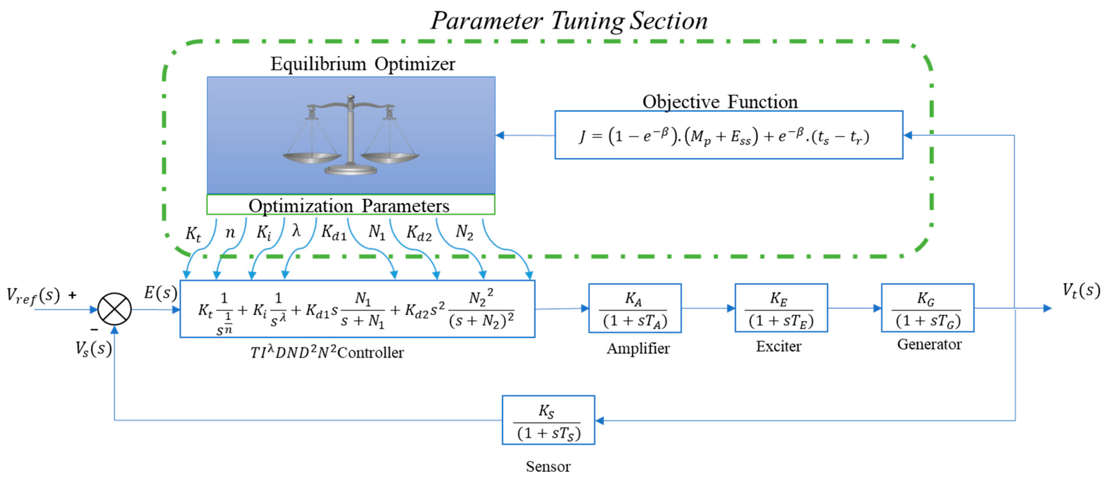
2. Modelling of the AVR System

The linearized transfer function model of AVR, which consists of four basic components such as amplifier, exciter, generator, and sensor is shown in Figure 1. For simplicity, nonlinearity and saturation are ignored in the AVR system. In Figure 1, $K_A$, $K_E$, $K_G$, and $K_S$ are the gain of amplifier, exciter, generator, and sensor, respectively, while $T_A$, $T_E$, $T_G$, and $T_S$ show the time constant of the amplifier, exciter, generator, and sensor, respectively. $V_{ref}$ denotes the reference voltage. $V_S$ is the output of the sensor, and E is the error signal obtained by subtracting $V_S$ from $V_{ref}$ ($V_{ref}-V_S$). $V_t$ represents the terminal voltage signal of the generator.

Table 1. Transfer functions and parameters of the AVR system components.

Units	Transfer Function	Range of Gain (K)	Range of Time Constant (Ts)	Gain Values Used (K)	Time Constants Used (Ts)
Amplifier	$G_A=\frac{K_A}{1+s{T}_A}$	10–40	0.02–0.1	10	0. 1
Exciter	$G_E=\frac{K_E}{1+s{T}_E}$	1–10	0.4–1	1	0.4
Generator	$G_G=\frac{K_G}{1+s{T}_G}$	0.7–1	1–2	1	1
Sensor	$G_S=\frac{K_S}{1+s{T}_S}$	0.9–1.1	0.001–0.06	1	0.01

gives the transfer functions of the components of the AVR system and the gain and time constants of these components. In the table, the values in the range of gain and range of time constant columns represent possible values, while the gain values used and time constants used columns show the values used in the study [9,10,11,12,13,14,21].

Equation (1) depicts the closed-loop transfer function of the AVR system achieved using the transfer functions of the components given in Figure 1 with the values given in Table 1.

$${\mathrm{G}}_{\mathrm{AVR}}=\frac{0.1\mathrm{s}+10}{0.0004{\mathrm{s}}^4+0.0454{\mathrm{s}}^3+0.555{\mathrm{s}}^2+1.51\mathrm{s}+11}$$

(1)

In order to evaluate the proposed controller in the time and frequency domain, first, it is necessary to analyse the AVR system without a controller in the time and frequency domain. Figure 2 demonstrates the step response of the terminal voltage of an AVR system without a controller. It can be seen that the terminal voltage of the AVR system without the controller does not settle at the reference position. Neither the overshoot with 65.72% nor the steady state error with 0.0909 p.u. are acceptable for AVR systems.

Figure 3 shows the Bode diagram of the AVR system without a controller, and

Table 2. Frequency response of the AVR system without a controller.

System	Peak Gain (dB)	Phase Margin (deg)	Delay Margin (s)
AVR (without controller)	11.8 (at 4.64 rad/s)	−5.43	0.994

gives the calculated frequency response according to the Bode diagram. As can be seen from the table, the peak gain of 11.8 dB is quite high, while the phase margin of 43 degrees and the delay margin of 0.994 s are low. In addition, it is seen that the bandwidth value is 6.78 rad/s, which indicates that the rise time shown in the time domain analysis is high. To bring this time and frequency domain specifications to acceptable levels, it is necessary to use a controller.

3. Control Methodologies

3.1. A Brief Overview of Fractional Calculus

Fractional calculus-based control systems have become increasingly common recently. In order to apply fractional order controllers (FOCs) to engineering systems, some numerical operations must be implemented. The continuous integro-differential agent ${}_a{}^{1}D{}_t^r$ is depicted in Equation (2).

$${}_a{}^{1}D{}_t^r=\left\{\begin{array}{c}\frac{d^r}{d{t}^r} R\left(r\right)>0,\\ 1 R\left(r\right)=0,\\ {{\displaystyle \int }}_a^t{\left(d\tau \right)}^{-r} R\left(r\right)<0.\end{array}\right.$$

(2)

In Equation (2), $\alpha$ and $t$ specify the bounds of operation. $r$ depicts the fractional order (FO) of the integro-differential operator ($r\in R$).

$$s^r\approx K_f{{\displaystyle \prod }}_{k=-N}^N\frac{s+w_k^{\prime }}{s+w_k}$$

(3)

In the study, ORA, which is used for the approximation required for real-time applications, was preferred. ORA is given in Equation (3), and poles, zeros, and gain of the filter are defined in Equation (4).

$$w_k=w_b{\left(\frac{w_h}{w_b}\right)}^{\frac{k+N+\frac{1}{2\left(1+r\right)}}{2N+1}}; w_k^{\prime }=w_b{\left(\frac{w_h}{w_b}\right)}^{\frac{k+N+\frac{1}{2\left(1-r\right)}}{2N+1}}; K_f=w_h^r$$

(4)

where (2N + 1) is the order of the analogue filter, and ($w_b,w_h$) represents the suitable range. Filter limits are taken as [10⁻³, 10³] in the paper.

FOCs are obtained by configuring the integer order controller, the PID controller, according to the fractional calculus base. The most basic of these FOCs are TID and FOPID controllers. TID controller is obtained by multiplying the proportional part of the PID with $“1/s^{\left(1/n\right)}”$. Thus, the part obtained after the process is called the “tilt” compensator. Although “n” is chosen specific to the problem, it is usually taken between 1 and 10. The integro-differential operators in the FOPID controller provide the FO feature. Transfer functions of PID, TID, and FOPID controllers are given in Equations (5)–(7).

$$C_{PID}=K_p+K_i\frac{1}{S}+K_{d}s$$

(5)

$$C_{TID}=K_t\frac{1}{s^{\frac{1}{n}}}+K_i\frac{1}{S}+K_{d}s$$

(6)

$$C_{FOPID}=K_p+K_i\frac{1}{s^{\lambda }}+K_d{s}^{\mu }$$

(7)

where $K_p$, $K_t$, $K_i$, and $K_d$ are the proportional, tilt, integral, and derivative gains, and λ and μ are the integro-differential operators.

The transfer functions of PIDD² and PIDA controllers, which are used in AVR systems and give better results than PID, are given in Equations (8) and (9) [21,31].

$$C_{PID{D}^2}=K_p+K_i\frac{1}{S}+K_{d}s+K_{d2}{s}^2$$

(8)

$$C_{PIDA}=K_p+\frac{K_i}{s}+\frac{K_{d}s}{s+d}+\frac{K_a{s}^2}{\left(s+d\right)\left(s+e\right)}$$

(9)

where $K_{d2}$ and $K_a$ are the second order derivative and accelerated gains, respectively. d and e are filter coefficients. Equation (10) is obtained as a result of polynomial simplification of Equation (9).

$$C_{PIDA}=\frac{K_a{s}^3+K_d{s}^2+K_{p}s+K_i}{s^3+\alpha s^2+\beta s}$$

(10)

where $a$ and $\beta$ are polynomial coefficients.

3.2. Proposed Controller

The fundamental of the proposed TI^λDND²N² controller is based on the hybridization of TID and PIDD². The final version of the proposed controller is obtained by adding fractional integral and two low-pass filters to this hybrid version. Researchers know that when controllers are used hybrid, they eliminate each other’s disadvantages, thus resulting in a more effective controller. In addition, it is known that the sensitivity of the controller increases as the tuning parameter increases. Therefore, the transfer function of the TI^λDND²N² controller with eight tuning parameters obtained is given in Equation (11).

$$C_{TIDN{D}^2{N}^2}=K_t\frac{1}{s^{\frac{1}{n}}}+K_i\frac{1}{s^{\lambda }}+K_{d1}s\frac{N_1}{s+N_1}+K_{d2}{s}^2\frac{N_2{}^2}{{\left(s+N_2\right)}^2}$$

(11)

where $K_t$, $K_i$, $K_{d1}$, and $K_{d2}$ are tilt, integral, first derivative, and second derivative gains. λ represents integro operator. $N_1$ and $N_2$ demonstrate the filter coefficients. Figure 4 shows the transfer function block diagram of the AVR system with TI^λDND²N² controller integrated with the optimization algorithm and objective function.

The error (E), which is the difference between the reference voltage and the voltage obtained from the sensor output, enters the proposed controller before entering the system. The output of the controller is also called the control input of the system and ensures that the voltage $V_t$ reaches the best time domain specifications. Detailed information about the optimization algorithm and objective function in the figure is given in the next sections.

Equation (12) gives the generalized closed-loop transfer function of the AVR system with controller.

$$G_{AVR,controller}=\frac{C_{controller} G_A{G}_E{G}_G}{1+C_{controller} G_A{G}_E{G}_G{G}_S}$$

(12)

$C_{controller}$ represents the transfer function of the controller used in the system. $G_A$, $G_E$, $G_G$, and $G_S$ are the transfer functions of amplifier, exciter, generator, and sensor, respectively, as given in Table 1.

4. Optimization Algorithm

The equilibrium optimizer algorithm is inspired from the dynamic mass balance, which defines the conservation of mass that leaves, enters, or generates in a control volume. EO was proposed by Faramarzi in 2020 [32]. A first-order differential equation of mass balance is depicted in Equation (13):

$$V\frac{dC}{dt}=Q{C}_{eq}-QC+G$$

(13)

where V represents the control volume, C defines the concentration of the control volume, and $V\frac{dC}{dt}$ depicts the variation ratio of mass in control volume. Q is the volumetric flow ratio entering and leaving the control volume. G represents the ratio of mass generation inside the control volume, and $C_{eq}$ is the concentration at equilibrium condition without production within the control volume.

First, $\frac{dC}{dt}$ given in Equation (13) is taken as a function of $\frac{Q}{V}$, and some adjustments are made by representing $\frac{Q}{V}$ with λ. At the end of these arrangements, the following equation is obtained, which expresses the balance between exploration and exploration.

$$F=\exp \left[-\lambda \left(t-t_0\right)\right]$$

(14)

where $t_0$ is the initial time depending on the integration interval.

4.1. Initialization

EO needs an initial population to start the optimization period. In the initialization part, the initial concentrations are designed in accordance with dimensions and the number of particles as given in Equation (15).

$$C_i^{initial}=C_{min}+ran{d}_i\left(C_{max}+C_{min}\right) i=1,2,\dots n$$

(15)

$C_i^{initial}$ denotes the primary concentration vector of the i-th particle. $C_{min}$ and $C_{max}$ are the minimum and maximum values for the dimensions, the $ran{d}_i$ vector changes randomly in the range [0, 1], and n represents the population number.

4.2. Equilibrium Pool and Candidates (Ceq)

In fact, the last convergence situation of the algorithm is the equilibrium state. In EO algorithm, there are five particles described as equilibrium candidates. Four of them are the best particles so far, and one of them is the mean of the four particles. Five particles constitute a vector named the equilibrium pool as follows:

$${\overrightarrow{C}}_{eq,pool}=\left\{ {\overrightarrow{C}}_{eq\left(1\right),} {\overrightarrow{C}}_{eq\left(2\right), } {\overrightarrow{C}}_{eq\left(3\right),} {\overrightarrow{C}}_{eq\left(4\right),} {\overrightarrow{C}}_{eq\left(ave\right) }\right\}$$

(16)

4.3. Exponential Term

Equation (17) is obtained by modifying Equation (14) and is a concentration update procedure.

$$\overrightarrow{F}=a_{1}sign\left(\overrightarrow{r}-0.5\right)\left[e^{-\overrightarrow{\lambda }{\left(1-\frac{Iter}{Ma{x}_{iter}}\right)}^{\left(a_2\frac{Iter}{Ma{x}_{iter}}\right)}}-1\right]$$

(17)

λ depicts a random vector between [0, 1]. $Iter$ and $Ma{x}_{iter}$ show the current and the maximum number of iterations. $a_1$ and $a_2$ are fixed values responsible for exploration and exploitation stages, respectively. In the study, $a_1$ and $a_2$ values are taken as 2 and 1, respectively. $a_1$ value should be increased to improve exploration performance. However, in this case, the exploitation performance decreases. Similarly, the $a_2$ value should be increased to improve exploitation performance. In this case, the exploration performance decreases. $\overrightarrow{r}$ is a random vector in the range of [0, 1], and $sign\left(\overrightarrow{r}-0.5\right)$ chooses the way of exploitation and exploration.

4.4. Generation Rate

The generation rate (G) ensures better results by improving the exploitation phase. It is given in Equation (18).

$$\overrightarrow{G}=\left\{\begin{array}{c}0.5r_1\left({\overrightarrow{C}}_{eq}-\overrightarrow{\lambda }\overrightarrow{C}\right) \overrightarrow{F} ,r_2\ge GP\\ 0 , r_2<GP\end{array}\right.$$

(18)

$r_1$ and $r_2$ are random numbers between [0, 1]. GP represents the probability of generation and is taken as 0.5. With this value, GP creates the best equilibrium between exploration and exploitation phases. Equation (19) is the updating process of the EO algorithm.

$$C={\overrightarrow{C}}_{eq}+\left(\overrightarrow{C}-{\overrightarrow{C}}_{eq}\right)\overrightarrow{F}+\frac{\overrightarrow{G}}{\overrightarrow{\lambda }V}\left(1-\overrightarrow{F}\right)$$

(19)

In Equation (19), the first term represents the equilibrium concentration, the second term is related to the exploration phase, and the third term is responsible for the exploitation phase. See [32] for details of the algorithm.

Table 3. Experimental parameters of the EO algorithm.

Parameters	Values/Ranges
Iteration number	100
Population number	50
Variables number	8
Constant controlling the exploration phase ($a_1$)	2
Constant controlling the exploitation phase ($a_2$)	1
Generation Probability (GP)	0.5
$r_1$, $r_2$	[0, 1]

gives the experimental specifications of the EO algorithm utilized in this study. Figure 5 demonstrates the flow diagram of the EO algorithm.

5. Objective Function

The objective function is defined as an equation that must be maximized or minimized during optimization in order to obtain the optimal reaction of the system under study [19]. Therefore, an efficient objective function is needed for better tuning the controller parameters. In our study, the objective function containing the time domain specifications is given as follows [33]:

$$J=\left(1-e^{-\beta }\right).\left(M_p+E_{ss}\right)+e^{-\beta }.\left(t_s-t_r\right)$$

(20)

where $\beta$ represents weighting factor, $M_p$ denotes overshoot, and $E_{ss}$ is steady state error. $t_s$ and $t_r$ are settling time and rise time, respectively. In the case of $\beta$ < 0.7, the settling and rise time decrease, and in the case of $\beta$ > 0.7, the overshoot and steady state error decrease. In order to provide a balance between the time domain specifications, $\beta$ is taken as 0.7 in our study. Optimization parameters are $K_t$, $K_i$, $K_{d1}$, $K_{d2}$, n, λ, $N_1$, and $N_2$ for the TI^λDND²N² controller. The lower and upper bounds of these parameters are LB = [0, 0, 0, 0, 1, 0.01, 10, 10] and UB = [3, 3, 3, 3, 10, 1.5, 500, 1000], respectively.

6. Results and Discussion

Brief information about the AVR system without a controller is explained in Section 2, and the graphs of step response and Bode plot are given in Figure 2 and Figure 3. In this section, performance comparisons of the proposed controller with other controllers, Bode plot analysis, and robustness tests on perturbed system parameters were performed, respectively. The attitude of the proposed controller under all these conditions was examined. The study was realized in MATLAB 2016a/Simulink environment. The specifications of the computer on which the study was conducted were Intel Core i5-4570 and 4 GB of RAM.

6.1. The Performance Achievement of the TI^λDND²N² Controller

In this section, the performance of the proposed controller is demonstrated by comparing it with PID-multiverse optimizer (MVO) [22], PID-equilibrium optimizer (EO) [23], PID-sine-cosine algorithm (SCA) [10], PID-tree seed algorithm (TSA) [34], PID-whale optimization algorithm (WOA) [12], PID water cycle algorithm (WCA) [11], PID-improved WOA (IWOA) [35], sigmoid PID nonlinear SCA [26], PIDA-local uni-modal sampling (LUS) [9], PIDA-teaching-learning-based optimization (TLBO) [9], PIDA-harmony search algorithm (HSA) [9], PIDA-WOA [12], PIDD²-particle swarm optimization (PSO) [21], PIDD²-EO [23], multi-term FOPID-RAO [24], FOPID-SCA [10], FOPID-chaotic yellow saddle goatfish algorithm (C-YSGA) [30], FOPID-hybrid simulated annealing—manta ray foraging optimization algorithm (hSA-MRFO) [14], FOPID-COA [18], FOPID-EO [23], FOPID-MVO [22], FOPID-Seagull optimization algorithm (SOA) [36], FOPID-chaotic black widow algorithm (ChBWO) [37], a reinforcement learning approach [38], sliding mode control [5], PID-Fuzzy TLBO [39], PID-Fuzzy PSO [39], RBF-NN with a Sugeno fuzzy logic based PID (GNFPID) [40], fractional variable order PID (FVOPID)-YSGA [41], and FVOPID-V2-YSGA [41].

Table 4. Parameters of compared controllers.

Method	${\mathit{K}}_{\mathit{p}}/{\mathit{K}}_{\mathit{t}}$	${\mathit{K}}_{\mathit{i}}$	${\mathit{K}}_{\mathit{d}1}$	${\mathit{K}}_{\mathit{d}2}$	$\mathit{n}/{\mathit{K}}_{\mathit{a}}$	λ/α	μ/β	${\mathit{N}}_1$	${\mathit{N}}_2$
TIλDND2N2 EO	2.1792	2.6626	1.5658	0.1365	2.3438	0.1099	--	36.2387	246.8546
PID IWOA [34]	0.8167	0.6898	0.2799	--	--	--	--	--	--
PID MVO [21]	0.5971	0.4057	0.1980	--	--	--	--	--	--
PID WCA [10]	0.6158	0.4410	0.2158	--	--	--	--	--	--
FOPID SOA [35]	0.9697	0. 4918	0. 2210	--	--	1.1522	1.1524	--	--
FOPID hSA-MRFO [13]	1.8931	0.8699	0.3595	--	--	1.0408	1.278	--	--
FOPID ChBWO [36]	2.8204	0.7387	0.428	--	--	1.1294	1.3558	--	--
PIDD2 EO [22]	3	2.0058	1.0936	0.0789	--	--	--	--	--
PIDD2 PSO [20]	2.7784	1.8521	0.9997	0.0739	--	--	--	--	--
PIDA WOA [11]	777.401	397.741	500.652	--	103.02	550.118	915.041	--	--
PIDA TLBO [8]	850	421.601	550	--	150	550	900	--	--

gives the parameters of the compared controllers. In the table, only the studies that make up the graph in Figure 6 are included.

Table 5. Comparative evaluation of different controllers in terms of transient response.

	Controller-Algorithm	${\mathit{T}}_{\mathit{s}}$ (s)	${\mathit{T}}_{\mathit{r}}$ (s)	${\mathit{M}}_{\mathit{p}}$ (%)
Proposed	TIλDND2N2-EO	0.0596	0.03752	0.4128
PID	PID MVO [22]	0.5074	0.3264	0.0018
	PID EO [23]	0.4478	0.2954	1.0004
	PID SCA [10]	0.665	0.3935	0.019
	PID TSA [34]	0.758	0.1310	15.57
	PID WOA [12]	2.1359	0.2152	7.2570
	PID WCA [11]	0.4620	0.3000	0.4760
	PID IWOA [35]	0.6420	0.2120	9.56
	Sigmoid PID Nonlinar SCA [26]	0.579	0.498	1.022
PIDA	PIDA LUS [9]	1.1725	0.3465	1.8049
	PIDA TLBO [9]	1.1023	0.2758	0.6332
	PIDA HSA [9]	1.09838	0.3073	0.4899
	PIDA WOA [12]	0.4996	0.3295	1.4087
PIDD2	PIDD2 PSO [21]	0.1635	0.0929	0.0027
	PIDD2 EO [23]	0.1399	0.0829	0.0041
FOPID	MFOPID RAO [24]	0.170	0.0965	0.01
	FOPID SCA [10]	0.2260	0.1660	2.4223
	FOPID C-YSGA [30]	0.2	0.1347	1.89
	FOPID hSA MRFO [14]	0.1909	0.1309	1.9765
	FOPID COA [18]	0.1474	0.1011	1.952
	FOPID EO [23]	0.4596	0.1442	0.1849
	FOPID MVO [22]	0.3493	0.1075	1.0295
	FOPID SOA [36]	0.4459	0.2745	0.1516
	ChBWO-FOPID [37]	0.1586	0.1101	1.2714
Hybrid Controllers	A reinforcement learning approach [38]	0.55	0.34	0.2064
	Sliding Mode Control [5]	0.8812	0.2998	0.08
	Fuzzy TLBO-PID [39]	0.86	0.73	0.0001
	Fuzzy PSO PID [39]	1.9500	1.3400	0.2510
	GNFPID [40]	1.3766	1.0024	0.0017
	YSGA FVOPID [41]	n/a	0.09820	0.71987
	YSGA FVOPID V2 [41]	n/a	0.09808	1.35453

n/a: Not available.

shows the comparative evaluation of different controllers such as PID, FOPID, PIDA PIDD², and hybrid controllers in terms of the transient response. According to Table 5, it is seen that the results obtained using FOPID-based studies are better than the results obtained using PID and PIDA-based studies. Among the reasons for this, it can be shown that the FOPID controller is fractional calculus-based and, accordingly, has two (λ,μ) extra tuning parameters.

It is seen that the same controllers give different results in different studies. The main reasons for this are the optimization methods used, different operating parameters of the artificial intelligence optimization algorithms, and objective functions used.

Additionally, it is seen that $T_s$, $T_r$, and $M_p$ are better in PIDD²-based studies than PID, PIDA, and FOPID-based studies. The contribution of the second order derivative part and the effect of its compatibility with AVR systems cannot be ignored.

On the other hand, considering the step function response of the $V_t$ output of the proposed TI^λDND²N² based AVR system, it is seen that the settling time ($T_s=0.0596 \mathrm{s}$) and rise time ($T_r=0.03752 \mathrm{s}$) are at much better levels than the compared controllers. According to the results of the systems with PID control, an approximately 10 times decrease is observed in the settling and rise times. Further, the maximum overshoot ($M_p=0.4128 \%$) is better than many of the methods compared and is well below the acceptable limit. In addition to the effect of the second-order derivative part in the controller, the effect of the tilted compensator and filters significantly increased the control performance.

Figure 6 demonstrates the step function response of the AVR system controlled by proposed controller in this paper and the proposed controllers in recently published papers. The numerical results given in Table 5 are displayed graphically in Figure 6. Accordingly, it is seen that AVR systems with PIDD² controller give better results than previously suggested controllers such as PID, FOPID, and PIDA. It can be clearly seen that the proposed controller is better than all the previously used controllers in terms of both the rise time and the speed of settling to the reference level for the V_t voltage output of the AVR.

6.2. Frequency Domain Analysis

Bode analysis is realized to examine the performance of the proposed controller in the frequency domain. Figure 7 demonstrates the Bode diagram of the AVR system controlled by TI^λDND²N².

Table 6. Frequency response of the AVR system obtained with different controllers.

Controller-Method	Peak Gain (dB)	Phase Margin (deg)	Delay Margin (s)
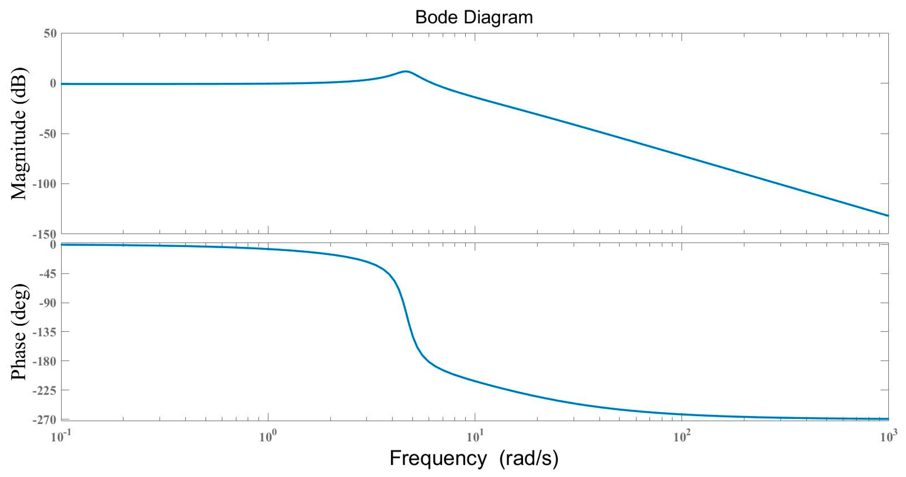
TIλDND2N2-EO	0. 0233 (at 2.16 rad/s)	175	1.14
PID-ABC [28]	2.87 (at 7.54 rad/s)	69.4	0.111
POD-PSO [28]	3.75 (at 7.16 rad/s)	62.2	0.103
PID-EO [23]	0.00178 (0.31 rad/s)	175	7.01
PID-WOA [12]	0.569 (n/a)	155	1.04
PIDD2- EO [23]	0 (0 rad/s)	180	Inf
PIDA-LUS [9]	0.159 (n/a)	162	2.42
FOPID-SOA [36]	0.0259 (n/a)	176	1.38
FOPID-SCA [29]	0.0379 (0.263 rad/s)	165	1.24
FOPID-EO [23]	0.0618 (0.242 rad/s)	177	7.34

n/a: Not available.

presents the frequency response of the AVR system with different controllers. The table demonstrates that the TI^λDND²N²-based AVR system has high stability in frequency domain with low peak gain (0.0233 dB at 2.16 rad/s), high phase margin (175 deg) and high bandwidth (55.7 rad/s). In addition, with a value of 1.14 s, the delay margin is competitive with other controllers. The fact that TI^λDND²N² has the highest bandwidth among the compared studies means that it has the lowest rise time. Another advantage of wide bandwidth is that it enables the system to accurately monitor random inputs. If the Bode diagram results are evaluated, the performance of the proposed controller on AVR systems in the time domain continues in the frequency domain.

6.3. Robustness Analysis

In AVR systems, deterioration in the design parameters may occur due to both load changes and external effects. Therefore, the attitude of $V_t$ voltage is investigated by changing the $T_A$, $T_E$, $T_G$, and $T_S$ parameters by $\pm$25% and $\pm$50%. Thus, the performance of the proposed controller is evaluated not only under normal operating conditions but also under perturbed system parameters.

Table 7. Time domain specifications of the AVR system at changed time constants values.

	Perturbation Variation (%)	Peak Value (p.u)	${\mathit{T}}_{\mathit{s}}$(s)	${\mathit{T}}_{\mathit{r}}$(s)	${\mathit{T}}_{\mathit{p}}$(s)
	Nominal Values	0.9937138	0.0596	0.03752	0.1827
$T_A$	−50	1.142358	0.2637	0.01808	0.0412
	−25	1.03247	0.15194	0.02686	0.05371
	+25	1.02067	0.2250	0.04915	0.16243
	+50	1.04847	0.2905	0.05987	0.17193
$T_E$	−50	1.27087	0.30788	0.01669	0.04075
	−25	1.07934	0.12966	0.02539	0.05257
	+25	1.00453	0.10158	0.05433	0.1996
	+50	1.01394	0.30182	0.07306	0.2133
$T_G$	−50	1.30404	0.13815	0.016417	0.04137
	−25	1.09113	0.11917	0.02512	0.05263
	+25	0.99731	0.11430	0.05603	0.75282
	+50	1.0029	0.14260	0.078498	0.72093
$T_S$	−50	0.99424	0.11751	0.04972	0.67725
	−25	0.99403	0.10542	0.04162	0.70737
	+25	1.030779	0.09614	0.035358	0.075396
	+50	1.06998	0.11272	0.033879	0.07659

demonstrates the time domain specifications of the AVR system controlled by the TI^λDND²N² on changed time-constant criterion.

As seen in the table, the maximum peak value is 1.30404 (when $T_G$ is dropped to −50%), the highest value of $T_s$ is 0.3079 s (when $T_E$ is dropped by −50%), and the maximum value of $T_r$ is 0.0785 s (when $T_G$ is raised by +50%).

Figure 8 depicts the step response of output of the AVR systems achieved after the deterioration in $T_A$, $T_E$, $T_G$, and $T_S$ parameters. As can be seen from the figure, the −50% change in $T_A$, $T_E$, and $T_G$ slightly increased the overshoot. In other cases, the proposed controller is almost unaffected. As can be seen from the figure, the proposed controller copes with the disturbances in the system.

7. Conclusions

This paper proposes a novel tilt-fractional order integral-derivative with second order derivative and low-pass filters controller, called TI^λDND²N² controller, to enhance the control ability of AVR systems. Thus, an excellent controller has been presented to the literature to provide sustainable voltage control. To optimize the eight parameters of the proposed controller, the EO algorithm, which has been successfully applied in engineering applications in recent years, has been used. The objective function used in the study consists of basic time domain specifications such as settling time, rise time, and overshoot. The superior performance of the proposed controller in terms of time domain results has been demonstrated by comparison with previously proposed PID, FOPID, PIDA, PIDD², and hybrid controllers for AVR systems. Then, Bode analysis is performed to examine its effectiveness in the frequency domain. According to the results obtained after Bode analysis, the proposed controller shows superior performance in the frequency domain. Finally, the results obtained for the perturbed system parameters are even better than the nominal operating conditions of other controllers. Thus, it has been seen that the proposed controller is successful even in unexpected situations in the system. All simulation results show that the proposed controller can be used in AVR systems with ease. In future studies, control structures can be studied to increase the control capability of AVR systems. If the studied controller has tuning parameters, the optimization algorithm can be hybridized, or a new objective function can be developed to tune these parameters well. In the studies, it is clear that controller development is the method that increases the control capability of AVR systems the most. Therefore, the improvement of controllers suitable for the structure of AVR systems forms the basis of future studies.

References

- Sedighizadeh, M.; Esmaili, M.; Eisapour-Moarref, A. Voltage and frequency regulation in autonomous microgrids using Hybrid Big Bang-Big Crunch algorithm. Appl. Soft Comput. 2017, 52, 176–189. [Google Scholar] [CrossRef]
- Boldea, I. Synchronous Generators, 2nd ed.; CRC Press: Boca Raton, FL, USA, 2016. [Google Scholar]
- Ula, A.; Hasan, A.R. Design and Implementation of a Personal Computer Based Automatic Voltage Regulator for a Synchronous Generator. IEEE Trans. Energy Convers. 1992, 7, 125–131. [Google Scholar] [CrossRef]
- Duman, S.; Yörükeren, N.; Altaş, İ. Gravitational search algorithm for determining controller parameters in an automatic voltage regulator system. Turk. J. Electr. Eng. Comput. Sci. 2016, 24, 2387–2400. [Google Scholar] [CrossRef] [Green Version]
- Furat, M.; Cucu, G.G. Design, Implementation, and Optimization of Sliding Mode Controller for Automatic Voltage Regulator System. IEEE Access 2022, 10, 55650–55674. [Google Scholar] [CrossRef]
- Gupta, T.; Sambariya, D.K. Optimal design of fuzzy logic controller for automatic voltage regulator. In Proceedings of the 2017 International Conference on Information, Communication, Instrumentation and Control (ICICIC), Indore, India, 17–19 August 2017; Volume 2018, pp. 1–6. [Google Scholar] [CrossRef]
- Yavarian, K.; Mohammadian, A.; Hashemi, F. Adaptive neuro fuzzy inference system PID controller for AVR system using SNR-PSO optimization. Int. J. Electr. Eng. Inform. 2015, 7, 394–408. [Google Scholar] [CrossRef]
- Tabak, A.; İlhan, İ. An effective method based on simulated annealing for automatic generation control of power systems. Appl. Soft Comput. 2022, 126, 109277. [Google Scholar] [CrossRef]
- Mosaad, A.M.; Attia, M.A.; Abdelaziz, A.Y.; Mosaad, A.M.; Attia, M.A.; Abdelaziz, A.Y.; Mosaad, A.M.; Attia, M.A. Comparative Performance Analysis of AVR Controllers Using Modern Optimization Techniques. Electr. Power Compon. Syst. 2018, 46, 2117–2130. [Google Scholar] [CrossRef]
- Bhookya, J.; Jatoth, R.K. Optimal FOPID / PID controller parameters tuning for the AVR system based on sine–cosine-algorithm. Evol. Intell. 2019, 12, 725–733. [Google Scholar] [CrossRef]
- Pachauri, N. Water cycle algorithm-based PID controller for AVR. COMPEL-Int. J. Comput. Math. Electr. Electron. Eng. 2020, 39, 551–567. [Google Scholar] [CrossRef]
- Mosaad, A.M.; Attia, M.A.; Abdelaziz, A.Y. Whale optimization algorithm to tune PID and PIDA controllers on AVR system. Ain Shams Eng. J. 2019, 10, 755–767. [Google Scholar] [CrossRef]
- Sikander, A.; Thakur, P. A new control design strategy for automatic voltage regulator in power system. ISA Trans. 2020, 100, 235–243. [Google Scholar] [CrossRef] [PubMed]
- Micev, M.; Calasan, M.; Ali, Z.M.; Hasanien, H.M.; Abdel, S.H.E. Optimal design of automatic voltage regulation controller using hybrid simulated annealing–Manta ray foraging optimization algorithm. Ain Shams Eng. J. 2021, 12, 641–657. [Google Scholar] [CrossRef]
- Miavagh, F.M.; Miavaghi, E.A.A.; Ghiasi, A.R.; Asadollahi, M. Applying of PID, FPID, TID and ITID controllers on AVR system using particle swarm optimization (PSO). In Proceedings of the 2015 2nd International Conference on Knowledge-Based Engineering and Innovation (KBEI), Tehran, Iran, 5–6 November 2015; pp. 866–871. [Google Scholar] [CrossRef]
- Shukla, H.; Nikolovski, S.; Raju, M.; Rana, A.S.; Kumar, P. A Particle Swarm Optimization Technique Tuned TID Controller for Frequency and Voltage Regulation with Penetration of Electric Vehicles and Distributed Generations. Energies 2022, 15, 8225. [Google Scholar] [CrossRef]
- Verma, S.K.; Devarapalli, R. Fractional order PIλDμ controller with optimal parameters using Modified Grey Wolf Optimizer for AVR system. Arch. Control Sci. 2022, 32, 429–450. [Google Scholar] [CrossRef]
- Moschos, I.; Parisses, C. A novel optimal PIλDND2N2 controller using coyote optimization algorithm for an AVR system. Eng. Sci. Technol. Int. J. 2022, 26, 100991. [Google Scholar] [CrossRef]
- Khan, I.A.; Alghamdi, A.S.; Jumani, T.A.; Alamgir, A.; Awan, A.B.; Khidrani, A. Salp Swarm Optimization Algorithm-Based Fractional Order PID Controller for Dynamic Response and Stability Enhancement of an Automatic Voltage Regulator System. Electronics 2019, 8, 1472. [Google Scholar] [CrossRef] [Green Version]
- Sikander, A.; Thakur, P.; Bansal, R.C.; Rajasekar, S. A novel technique to design cuckoo search based FOPID controller for AVR in power systems R. Comput. Electr. Eng. 2018, 70, 261–274. [Google Scholar] [CrossRef]
- Sahib, M.A. A novel optimal PID plus second order derivative controller for AVR system. Eng. Sci. Technol. Int. J. 2015, 18, 194–206. [Google Scholar] [CrossRef] [Green Version]
- Tabak, A. Maiden application of fractional order PID plus second order derivative controller in automatic voltage regulator. Int. Trans. Electr. Energy Syst. 2021, 31, e13211. [Google Scholar] [CrossRef]
- Tabak, A. A novel fractional order PID plus derivative (PIλDµDµ2) controller for AVR system using equilibrium optimizer. COMPEL-Int. J. Comput. Math. Electr. Electron. Eng. 2021, 40, 722–743. [Google Scholar] [CrossRef]
- Paliwal, N.; Srivastava, L.; Pandit, M. Rao algorithm based optimal Multi-term FOPID controller for automatic voltage regulator system. Optim. Control Appl. Methods 2022, 43, 1707–1734. [Google Scholar] [CrossRef]
- Agwa, A.; Elsayed, S.; Ahmed, M. Design of Optimal Controllers for Automatic Voltage Regulation Using Archimedes Optimizer. Intell. Autom. Soft Comput. 2021, 31, 799–815. [Google Scholar] [CrossRef]
- Suid, M.H.; Ahmad, M.A. Optimal tuning of sigmoid PID controller using Nonlinear Sine Cosine Algorithm for the Automatic Voltage Regulator system. ISA Trans. 2022, 128, 265–286. [Google Scholar] [CrossRef]
- Jumani, T.A.; Mustafa, M.W.; Zohaib, H.; Rasid, M.M.; Saeed, M.S.; Memon, M.M.; Khan, I.; Nisar, K.S. Jaya optimization algorithm for transient response and stability enhancement of a fractional-order PID based automatic voltage regulator system. Alex. Eng. J. 2020, 59, 2429–2440. [Google Scholar] [CrossRef]
- Gozde, H.; Taplamacioglu, M.C. Comparative performance analysis of artificial bee colony algorithm for automatic voltage regulator (AVR) system. J. Frankl. Inst. 2011, 348, 1927–1946. [Google Scholar] [CrossRef]
- Ayas, M.S.; Sahin, E. FOPID controller with fractional filter for an automatic voltage regulator. Comput. Electr. Eng. 2020, 90, 106895. [Google Scholar] [CrossRef]
- Micev, M.; Ćalasan, M.; Oliva, D. Fractional Order PID Controller Design for an AVR System Using Chaotic Yellow Saddle Goatfish Algorithm. Mathematics 2020, 8, 1182. [Google Scholar] [CrossRef]
- Puangdownreong, D. Application of Current Search to Optimum PIDA Controller Design. Intell. Control Autom. 2012, 3, 303–312. [Google Scholar] [CrossRef] [Green Version]
- Faramarzi, A.; Heidarinejad, M.; Stephens, B.; Mirjalili, S. Equilibrium optimizer: A novel optimization algorithm. Knowl.-Based Syst. 2020, 191, 105190. [Google Scholar] [CrossRef]
- Gaing, Z. A Particle Swarm Optimization Approach for Optimum Design of PID Controller in AVR System. IEEE Trans. Energy Convers. 2004, 19, 384–391. [Google Scholar] [CrossRef] [Green Version]
- Kose, E. Optimal Control of AVR System with Tree Seed Algorithm-Based PID Controller. IEEE Access 2020, 8, 89457–89467. [Google Scholar] [CrossRef]
- Habib, S.; Abbas, G.; Jumani, T.A.; Bhutto, A.A.; Mirsaeidi, S.; Ahmed, E.M. Improved Whale Optimization Algorithm for Transient Response, Robustness, and Stability Enhancement of an Automatic Voltage Regulator System. Energies 2022, 15, 5037. [Google Scholar] [CrossRef]
- Jegatheesh, A.; Thiyagarajan, V.; Selvan, N.B.M.; Raj, M.D. Voltage Regulation and Stability Enhancement in AVR System Based on SOA-FOPID Controller. J. Electr. Eng. Technol. 2023, 1–14. [Google Scholar] [CrossRef]
- Munagala, V.K.; Jatoth, R.K. Improved fractional PIλDμ controller for AVR system using Chaotic Black Widow algorithm. Comput. Electr. Eng. 2022, 97, 107600. [Google Scholar] [CrossRef]
- Ayas, M.S.; Sahin, A.K. A reinforcement learning approach to Automatic Voltage Regulator system. Eng. Appl. Artif. Intell. 2023, 121, 106050. [Google Scholar] [CrossRef]
- Priyambada, S.; Sahu, B.K.; Mohanty, P.K. Fuzzy-PID controller optimized TLBO approach on automatic voltage regulator. In Proceedings of the 2015 International Conference on Energy, Power and Environment: Towards Sustainable Growth (ICEPE), Shillong, India, 12–13 June 2015; IEEE: Piscateville, NJ, USA, 2015. [Google Scholar]
- Al Gizi, A.J.H.; Mustafa, M.W.; Al-geelani, N.A.; Alsaedi, M.A. Sugeno fuzzy PID tuning, by genetic-neutral for AVR in electrical power generation. Appl. Soft Comput. J. 2015, 28, 226–236. [Google Scholar] [CrossRef] [Green Version]
- Oziablo, P.; Mozyrska, D.; Wyrwas, M. Fractional-variable-order digital controller design tuned with the chaotic yellow saddle goatfish algorithm for the AVR system. ISA Trans. 2022, 125, 260–267. [Google Scholar] [CrossRef]