Optimal Scheduling of Reservoir Flood Control under Non-Stationary Conditions

Abstract

To improve reservoir flood control and scheduling schemes under changing environmental conditions, we established an adaptive reservoir regulation method integrating hydrological non-stationarity diagnosis, hydrological frequency analysis, design flood calculations, and reservoir flood control optimization scheduling and applied it to the Chengbi River Reservoir. The results showed that the peak annual flood sequence and the variation point of the annual maximum 3-day flood sequence of the Chengbi River Reservoir was in 1979, and the variation point of the annual maximum 1-day flood sequence was in 1980. A mixed distribution model was developed via a simulated annealing algorithm, hydrological frequency analysis was carried out, and a non-stationary design flood considering the variation point was obtained according to the analysis results; the increases in the flood peak compared to the original design were 4.00% and 8.66%, respectively. A maximum peak reduction model for optimal reservoir scheduling using the minimum sum of squares of the downgradient flow as the objective function was established and solved via a particle swarm optimization algorithm. The proposed adaptive scheduling scheme reduced discharge flow to 2661 m³/s under 1000-year flood conditions, and the peak reduction rate reached 60.6%. Furthermore, the discharge flow was reduced to 2661 m³/s under 10,000-year flood conditions, and the peak reduction rate reached 65.9%.

1. Introduction

As one of the types of natural disaster that occur most frequently, cause the most serious damage, and have the widest impact globally, floods have undergone obvious alterations in frequency, spatial and temporal distribution, and severity under the influence of climate and sub-surface changes [1]. In recent years, climate change and human activities have intensified, and hydrological conditions have changed significantly. The incoming flood sequences of many reservoirs no longer meet the assumption of stationarity, causing serious challenges for the original calculation methods of flood design, reservoir design, and operation scheduling. For instance, the use of traditional hydrological frequency calculation methods to analyze hydrological sequences under changing environmental conditions may result in less reliable calculation results and even the distortion of flood frequency design [2,3]. A reservoir scheduling plan created based on these results may lead to inadequate reservoir function or increase a reservoir’s safety risk due to the overestimation of the design’s ability to withstand flooding. Therefore, diagnosing hydrological non-stationarity characteristics, processing hydrological non-stationarity sequences, and establishing a scheduling method that adapts to non-stationary conditions and fully exploits the benefits of reservoir design are important issues that need to be addressed.

Diagnosing the variability in hydrological series, mainly through trend variability tests, mutation variability tests, and periodicity tests, is the first task to carry out in frequency analyses [4]. In terms of mutation variability diagnosis, Pettitt’s method [5], which was improved and refined by subsequent researchers, has become one of the most common methods used by scholars to find the mutation points of hydrological series. Inclan et al. [6] proposed a mutation variability diagnosis model based on the ICSS model, which was applicable to independent time series and could be used to analyze multi-point mutation variability problems. Rodionov et al. [7] classified common mean–mutation diagnostic methods into five categories: parametric or nonparametric test methods, curve fitting methods, CUSUM methods, and sequential analysis methods. Villarini et al. [8] verified that Pettitt’s method did not require the assumption that the series obeyed a specific distribution, and their test results regarding flood frequency distribution in the Midwest of the United States were robust and reliable. Due to the instability of a single diagnostic method, Xie et al. [9] constructed a hydrological variability diagnostic system from the statistical point of view that integrated trend and mutation variability, synthesized each diagnostic method by assigning weights, determined the year of variability and the variability form of a hydrological series by calculating the integrated weights and efficiency coefficients, and was then combined with physical cause analysis to finally arrive at diagnostic results. Hydrological variability diagnosis is commonly used as a stand-alone diagnostic method, which introduces a high degree of uncertainty into the results. The hydrological variability diagnostic system could greatly improve the reliability and accuracy of hydrological sequence variability diagnosis compared with a single diagnostic method.

Hydrological frequency calculation is closely related to the planning, design, operation, and management of water conservancy projects [10]. Therefore, considering the severe challenge of applying the traditional hydrological frequency calculation method based on the consistency assumption, the need to determine a frequency calculation method applicable to non-stationary hydrological sequences is urgent. At present, the main methods for the frequency analysis of non-stationary hydrological sequences are the reduction, time-varying moment [11], conditional probability model [12], and mixed-distribution model methods. The mixed-distribution model method effectively avoids the shortcomings of the series-reconstruction-based method and is often used for calculating the frequency of non-stationary hydrological series with obvious seasonal characteristics and different physical causes. The early mixed-distribution model was simply a curve-fitting process. Potter et al. [13] concluded in their study of flood frequency curves that the dog’s leg shape of the frequency curve was the result of flood series arising from different totals. Singh et al. [14] used the mixed-distribution model method to analyze the frequency of about 600 flood series in the United States and other countries and considered the probability distribution of the observed flood series as a mixture of the probabilities of two log-normal distributions, thus improving the fit. The mixed-distribution model only became widely used in hydrologic frequency studies after 1992, when it was demonstrated and improved upon by Wang and Singh [15]. Alila et al. [16] applied the mixed-distribution method to the frequency analysis of a long series of floods in the Gila River Basin in central Arizona and introduced a means of selecting the most reasonable distribution function in flood frequency analysis. Cheng Jingqing et al. [17] combined variational diagnosis theory and the hybrid distribution model method to analyze the frequency of runoff series in northern Shaanxi and Guanzhong, and the study showed that the mixed distribution model method was an effective way to analyze the frequency of non-stationary hydrological series. For most reservoirs, the design flood process is modeled using a hydrological frequency method based on the assumption of stationarity, which can limit the reservoir’s flood control function or increase the reservoir’s flood control risk [18]. Therefore, the flood process must be modeled under changing environments based on a more reasonable hydrological frequency method, facilitating the flood control scheduling of reservoirs.

Reservoir flood control scheduling is necessary not only to ensure the safety of dams, but also to solve the problem of contradictions between the supply and demand of water resources. It is important to study methods of flood control scheduling for reservoirs in order to fully exploit reservoirs’ storage function; improve the benefits of reservoirs in terms of flood control, irrigation, and water supply; promote sustainable development; and reduce flood losses [19]. According to various theoretical methods, flood control scheduling can be divided into conventional scheduling and optimal scheduling. Conventional scheduling typically uses the inlet flow or actual reservoir level as the criterion for determining reservoir discharge flow and formulates scheduling rules based on relevant management experience. This method is simple to implement and convenient to manage, but it cannot make full use of flood resources and has certain defects [20]. However, optimal scheduling can coordinate various objectives of reservoir operation, which is crucial for safely operating and maximizing the benefits of reservoirs. For example, Foufoula et al. [21] used a gradient dynamic planning method to design a scheduling model for the optimal scheduling of a reservoir group, which improved the accuracy of the calculation results. Oliveira et al. [22] used genetic algorithms to develop improved scheduling rules in a reservoir scheduling study. Valeriano et al. [23] combined a heuristic algorithm searching for the global optimal solution with a distributed hydrological model to effectively reduce the downstream flood flow, demonstrating the feasibility of heuristic algorithms in flood control scheduling applications. Trivedi et al. [24] proposed a time-varying elite mutation multi-objective particle swarm optimization algorithm for the derivation and performance evaluation of optimal reservoir operation strategies. Ehteram et al. [25] combined a bat algorithm with a particle swarm optimization algorithm to optimize the parameters of the Muskingum model for accurate flood scheduling in three case studies in the USA and UK. These studies effectively demonstrated that optimization algorithms could be used for the optimal scheduling of reservoir flood control but focused on stationarity flood processes.

In summary, many scholars have conducted research on hydrological non-stationarity diagnosis, hydrological frequency analysis, and reservoir flood control optimization scheduling and have produced abundant results. However, this study established an adaptive regulation method for reservoirs integrating hydrological non-stationarity diagnosis, hydrological frequency analysis, design flood calculation, and reservoir flood control optimization scheduling and applied it to research in Chengbi River Reservoir, aiming to quantitatively analyze the influence of human activities on floods in the basin and reduce the adverse effects of environmental changes on incoming floods by optimizing the scheduling methods of existing water conservancy projects in the basin. The purpose of this study was to propose a reservoir scheduling plan to maximize the flood control benefits under the current conditions and to ensure the expected benefits of the reservoir. To the best of our knowledge, few previous studies have combined hydrological non-stationarity diagnosis, hydrological frequency analysis, and reservoir flood control optimization scheduling to conduct research on the optimal scheduling of reservoir flood control under non-stationarity conditions, indicating that this paper has the potential to fill a significant research gap.

2. Study Area and Project Overview

2.1. Study Area

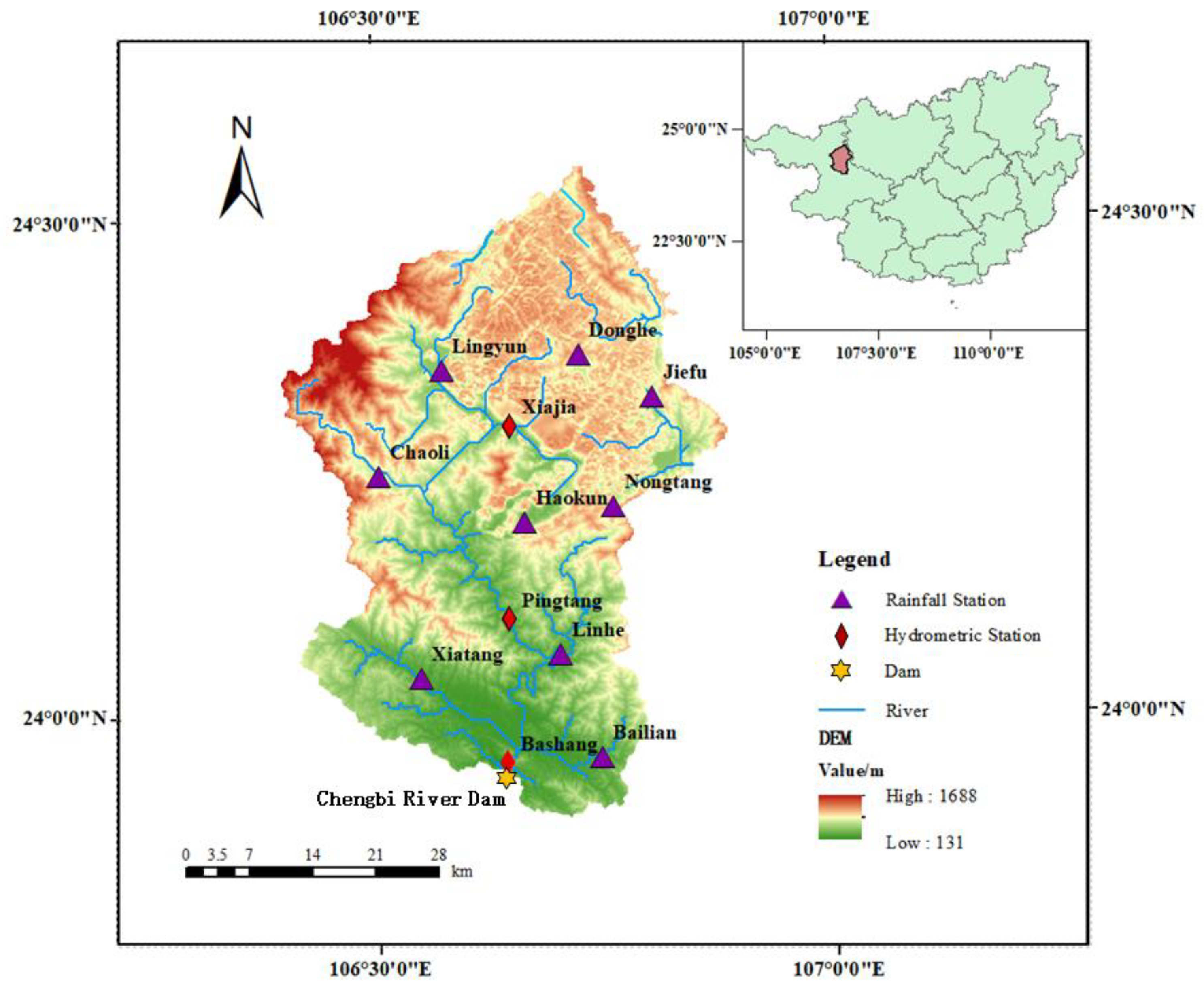
The Chengbi River originates from the eastern foot of Qinglong Mountain within Lingyun County, located to the northeast of Baise city, Guangxi district, China. The geographical location of the Chengbi River watershed is shown in Figure 1. In recent years, the impacts of climate change and human activities have become of increasing concern in the Chengbi River [26]. Climate change can bring fluctuations in precipitation and temperature, which affect the hydrological cycle and runoff evolution processes. Human activities can change the sub-surface conditions, directly or indirectly affecting the runoff [27]. Therefore, scientifically and rationally analyzing the effects of climate change and human activities on the Chengbi River Basin is a key issue.

2.2. Project Overview

Chengbi River Reservoir is a large type I water conservancy pivot project with comprehensive functions including power generation, flood control, fish farming, water supply, and multi-year regulation performance. It is one of the most representative earth and stone dam reservoirs in Guangxi [28]. Located downstream of Chengbi River Reservoir, the city of Baise is an important platform for China and ASEAN in their joint promotion of the ‘Belt and Road’ initiative, which is of great significance for driving the rapid development of the regional economy. Therefore, the Chengbi River Reservoir has a long history of research and was a suitable reservoir for validating the reliability of our methodology [29]. The engineering characteristics of the Chengbi River Reservoir are shown in

Table 1. Engineering characteristics of the Chengbi River Reservoir.

Category	Characteristic	Unit	Value
Hydrography	Catchment area	km2	2000
	Design flood standard	P (%)	0.1
	Design flood peak flow	m3/s	6460
	Calibration flood standard	P (%)	0.01
	Calibration flood peak flow	m3/s	7980
Reservoir	Design flood level	m	187.96
	Calibration flood level	m	189.29
	Flood limit level	m	184.5
	Dead level	m	167
	Total reservoir capacity	Million cubic meters (MCM)	1121
	Beneficial reservoir capacity	Million cubic meters (MCM)	600
	Dead storage capacity	Million cubic meters (MCM)	380
	Design flood maximum discharge	m3/s	2940
	Calibration flood maximum discharge	m3/s	3570
Dam	Top of dam elevation	m	190.4
	Maximum dam height	m	70.4
	Length of dam top	m	425
Spillway	Type		WES practical weir
	Weir top elevation	m	176
	Net width of overflow leading edge	m	4 × 12
	Design flood flow	m3/s	2300
	Calibration flood flow	m3/s	3580

.

2.3. Research Materials

In 1963, a reservoir station was set up in Chengbi River Reservoir to collect its annual operation data. Based on the Chengbi River Reservoir water level–capacity curve and the outflow from the reservoir, the annual maximum flood peak and annual maximum 1- and 3-day flood series of the reservoir for a total of 57 years from 1963 to 2019 were deduced and used as the basic data.

The corresponding water level–capacity and water level–discharge flow curves for the Chengbi River Reservoir are shown in Figure 2.

3. Methodology

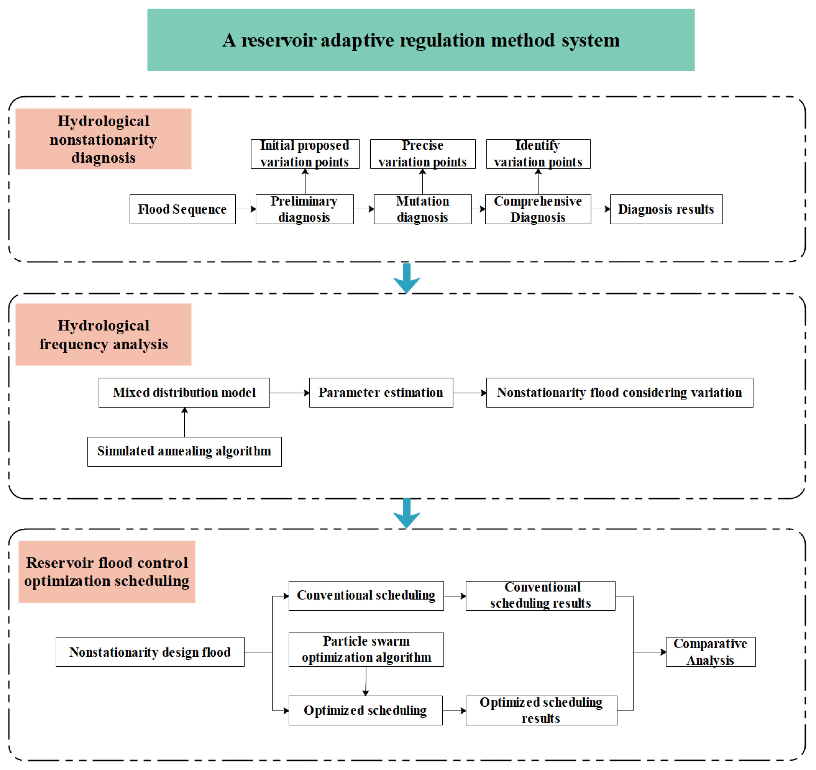
In order to represent the approach of this study more accurately, a flow chart is shown in Figure 3.

The main methods used in this study could be divided into three categories: (1) hydrological non-stationarity diagnosis methods, including preliminary, trend, mutation, and comprehensive diagnosis; (2) non-stationary flood sequence frequency analysis methods, including a mixed distribution model and a simulated annealing algorithm for non-stationary floods; (3) reservoir flood control optimization scheduling methods, including a reservoir flood control optimization scheduling model and particle swarm optimization algorithm. Due to limitations of space, only a few of these methods are briefly described below.

3.1. Hydrological Non-Stationarity Diagnosis Method

Hydrological non-stationarity diagnosis is a prerequisite for engineering design. First, the process line, sliding average, and Hurst coefficient methods were used to achieve a preliminary diagnosis of the hydrological sequences and determine whether they featured variations. If variability was identified, we had to further diagnose and analyze the mutability and trends. The trend diagnosis methods used in this study included the Spearman and Kendall rank order tests, and the mutability diagnosis methods included the sliding tour test, sliding rank sum test, Brown–Forsythe method, sliding t-test, ordered clustering method, and Lee–Heghinan test. After the results were obtained by the above methods, the most likely variation points were determined using the integrated diagnosis method.

3.1.1. Mutation Diagnosis

The purpose of mutation diagnosis is to identify the year in which the mutation of each sequence occurred. In order to enhance the persuasive power of variation identification, several tests with a higher weight in the traditional hydrological non-stationarity diagnosis system were selected in this study, including the sliding tour test, sliding rank sum test, Brown–Forsythe method, sliding t-test, ordered clustering method, Lee–Heghinan test, sliding F-test, and Mann–Kendall method. By calculating the combined weights of the diagnostic results of each test, the year with the largest combined weight was determined as the most likely year of variation. The calculation formulae and weight coefficients of each test are shown in

Table 2. Calculation formulae of mutation variation diagnosis methods.

Diagnosis Method	Formula	Weight
Sliding tour test	$\mathrm{U}=(\mathrm{K}-(1+\frac{2{\mathrm{n}}_1{\mathrm{n}}_2}{\mathrm{n}}\left)\right)/\sqrt{\frac{2{\mathrm{n}}_1{\mathrm{n}}_2(2{\mathrm{n}}_1{\mathrm{n}}_2-\mathrm{n})}{{\mathrm{n}}^2(\mathrm{n}-1)}}$	0.2280
Sliding rank sum test	$\mathrm{U}=(\mathrm{W}-\frac{{\mathrm{n}}_1({\mathrm{n}}_1+{\mathrm{n}}_2+1)}{2})/\sqrt{\frac{{\mathrm{n}}_1{\mathrm{n}}_2({\mathrm{n}}_1+{\mathrm{n}}_2+1)}{12}}$	0.1634
Brown–Forsythe method	$\mathrm{F}={\displaystyle \sum _{\mathrm{i}=1}^{\mathrm{m}}}{\mathrm{n}}_{\mathrm{i}}{({\mathrm{x}}_{\mathrm{i}}-{\mathrm{x}}_{\mathrm{N}})}^2/{\displaystyle \sum _{\mathrm{i}=1}^{\mathrm{m}}}(1-{\mathrm{n}}_{\mathrm{i}}/\mathrm{N}){\mathrm{s}}_{\mathrm{i}}^2$	0.1429
Sliding t-test	$T=(\overline{{\mathrm{x}}_1}+\overline{{\mathrm{x}}_2})/{\mathrm{S}}_{\mathrm{w}}{(\frac{1}{{\mathrm{n}}_1}+\frac{1}{{\mathrm{n}}_2})}^{1/2}$	0.1340
Ordered clustering method	$S_n^{\ast }=\underset{1\le \mathsf{\tau }\le \mathrm{n}-1}{\min }\{{\mathrm{S}}_{\mathrm{n}}(\mathsf{\tau })\}\mathrm{cc}$	0.1321
Lee–Heghinan method [30]	$f (\mathsf{\tau }/{\mathrm{x}}_1,{\mathrm{x}}_1,\dots ,{\mathrm{x}}_{\mathrm{n}})=\mathrm{k}{\left[\frac{\mathrm{n}}{\mathsf{\tau }(\mathrm{n}-\mathsf{\tau })}\right]}^{1/2}\left[\mathrm{R}\right(\mathsf{\tau }){]}^{-(\mathrm{n}-2)/2}$	0.0954
Sliding F-test	$\underset{1\le \mathsf{\tau }\le \mathrm{n}-1}{\max }\{\mathrm{f} (\mathsf{\tau }/{\mathrm{x}}_1,{\mathrm{x}}_2,\dots ,{\mathrm{x}}_{\mathrm{n}}\left)\right\}>{\mathrm{F}}_{\mathsf{\alpha }}$	0.0652
Mann–Kendall method	$U{B}_k=-U{F}_k$	0.0390

.

3.1.2. Comprehensive Diagnosis

The comprehensive diagnosis was based on the conclusions of the trend and mutation diagnoses, combined with the analysis of the physical factors in the study area. Then, the heuristic segmentation algorithm was used to test and review the final variation points. The computational principle of the heuristic segmentation algorithm is briefly described below [31].

For a time series $X$ with sample size $N$ and assuming the split point $i$, the combined deviation $S_D\left(i\right)$ for point $i$ is calculated as

$$S_D\left(i\right)={\left(\frac{\left(N_1-1\right)S_1^2+\left(N_2-1\right)S_2^2}{N_1+N_2-2}\right)}^{1/2}{\left(\frac{1}{N_1}+\frac{1}{N_2}\right)}^{1/2},$$

(1)

where $N_1$ and $N_2$ represent the numbers of sequences to the left and right of point $i$, respectively, and $s_1\left(i\right)$ and $s_2\left(i\right)$ represent the standard deviations of sequences to the left and right of point $i$, respectively.

In the above formula, $T\left(i\right)$ reflects the degree of difference between the left and right partial series means at point $i$, which is calculated as follows:

$$\begin{array}{c}T\left(i\right)=\left|\frac{{\mu }_1\left(i\right)-{\mu }_2\left(i\right)}{S_D}\right|,\end{array}$$

(2)

where ${\mu }_1\left(i\right)$ and ${\mu }_2\left(i\right)$ represent the averages of the left and right parts of the sequence at point $i$, respectively.

The larger the $T$ value, the greater the degree of difference between the left and right sides of the series at that point. $P\left(T_{\max }\right)$ denotes the statistical significance probability corresponding to the maximum value $T_{\max }$ for each $T$ value, which is calculated as follows:

$$\begin{array}{c}P\left(t_{\max }\right)\approx \{{1-I_{ \left[v/\left(v+t_{\max }^2\right) \right]}\left(\delta v,\delta \right)\}}^{\eta }cc,\end{array}$$

(3)

where $N$ denotes the length of the sequence, $v=N-2$, $\eta =4.19\ln N-11.54$, $\delta =0.40$, and $I_x(a,b)$ is the incomplete $\beta$ function.

3.2. Frequency Analysis Method for Non-Stationary Flood Sequences

Mixed Distribution Model and Simulated Annealing Algorithm

In 1991, Singh [15], an American hydrological scientist, proposed the mixed distribution model, which has since been continuously improved and developed, gradually gaining the attention of domestic and foreign hydrologists, and is becoming widely used in flood frequency analysis under non-coherent conditions. The mixed distribution method is directly based on the extreme-value sample series of non-coherent distribution for frequency analysis, assuming that this extreme-value sample series comprises several sub-distributions with the following form:

$$\begin{array}{c}F\left(x\right)={\alpha }_1{F}_1\left(x\right)+{\alpha }_2{F}_2\left(x\right)+\dots +{\alpha }_k{F}_k\left(x\right),\end{array}$$

(4)

where $F_1\left(x),F_2\right(x),\dots ,F_k\left(x\right)$ are the cumulative probability distribution functions of the $k$ sub-distributions, and $a_1,a_2,\dots ,a_k$ are the weight coefficients of each sub-series, satisfying $a_1+a_2+\cdots +a_k=1$.

In order to reduce the complexity of parameter estimation, the general assumption is that the mixed distribution comprises two sub-distributions. Due to the paucity of measured hydrological series in this study area, one of the most significant mutations was considered, i.e., the hydrological series was divided into two sub-series. Therefore, a mixed distribution model containing two sub-series was used. The basic principle is explained below.

Consider the non-stationary flood sequence $X$ with sample size $n$ and its variation point location $\tau$. The total sequence $X$ is divided into two sub-sequences, $X_1$ and $X_2$, where the sample length of sub-sequence $X_1$ is $n_1=\tau$ and its probability density function is $f_1\left(x\right)$; for sub-sequence $X_2$, the sample length is $n_2=n-\tau$ and the probability density function is $f_2\left(x\right)$. Then, the probability density function $f\left(x\right)$ of the total sequence $X$ is

$$\begin{array}{c}f\left(x\right)=\alpha f_1\left(x\right)+\left(1-\alpha \right)f_2\left(x\right),\end{array}$$

(5)

where $\alpha$ and $\left(1-\alpha \right)$ are the sub-series weight coefficients.

According to the ‘Specification for Calculation of Flood for Water Conservancy and Hydropower Engineering Design’ (SL44-2006) [32], the hydrological variables had to be fitted with a Pearson type III (P-III) curve for distribution. Suppose that the sub-series $X_1 \mathrm{and} X_2$ are subject to P-III distribution; then, $f_1\left(x\right),f_2\left(x\right)$ can be expressed as

$$f_1\left(x\right)=\frac{{\beta }_1^{{\alpha }_1}}{\Gamma \left({\alpha }_1\right)}{\left(x-{\alpha }_{01}\right)}^{{\alpha }_1-1}{e}^{-{\beta }_1\left(x-{\alpha }_{01}\right)}$$

(6)

$$f_2\left(x\right)=\frac{{\beta }_2^{{\alpha }_2}}{\Gamma \left({\alpha }_2\right)}{\left(x-{\alpha }_{02}\right)}^{{\alpha }_2-1}{e}^{-{\beta }_2\left(x-{\alpha }_{02}\right)}$$

(7)

Thus, the formula for calculating the theoretical frequency of the mixed distribution over the system frequency could be expressed as

$$\begin{array}{c}F\left(x\right)=\alpha \left[\frac{{\beta }_1^{{\alpha }_1}}{\Gamma \left({\alpha }_1\right)}{\int }_x^{+\infty }{\left(t-{\alpha }_{01}\right)}^{{\alpha }_1-1}{e}^{-{\beta }_1\left(t-{\alpha }_{01}\right)}dt\right]+(1-\alpha )\left[\frac{{\beta }_2^{{\alpha }_2}}{\Gamma \left({\alpha }_2\right)}{\int }_x^{+\infty }{\left(t-{\alpha }_{02}\right)}^{{\alpha }_2-1}{e}^{-{\beta }_2\left(t-{\alpha }_{02}\right)}dt\right].\end{array}$$

(8)

The parameters ${\alpha }_i,{\beta }_i$, and ${\alpha }_{0i} (i=1,2)$ could be expressed by the mean value of the statistical parameter $E{X}_i$, the coefficient of variation $C_{\mathrm{vi}}$, and the bias coefficient $C_{\mathrm{si}}$, which were calculated as follows: $E{X}_i={\alpha }_{0i}+{\alpha }_i/{\beta }_i,C_{\mathrm{vi}}=\sqrt{{\alpha }_i}/({\beta }_i{\alpha }_{0i}+{\alpha }_i),C_{\mathrm{si}}=2/\sqrt{{\alpha }_i}$. It followed that the parameters to be estimated in the mixed distribution model were $\alpha ,E{X}_1,C_{v1},C_{s1},E{X}_2,C_{v2}$, and$C_{s2}$.

The simulated annealing algorithm is highly suitable for finding the approximate global optimal solution of combinatorial optimization problems due to its robustness and simplicity of use [33]. As shown in Equation (8), seven parameters had to be estimated in the mixed distribution model. The simulated annealing algorithm was used to solve the mixed distribution model, and the measured hydrological data of each hydrological station in the Chengbi River Basin were combined to determine a $C_s/C_v$value variation range of [2.5, 3.5] as the constraint and the absolute values of the frequency deviation and minimum frequency as the objective function to estimate the model parameters [17,34].

3.3. Reservoir Flood Control Optimization Scheduling Method

3.3.1. Reservoir Flood Control Optimization Scheduling Model

The purpose of reservoir flood control scheduling is to maximize the use of a reservoir’s flood control capacity and minimize the damage caused by flooding in the downstream protection zone while safeguarding the safety of the dam [35]. In this study, according to the requirements of Chengbi River Reservoir, a maximum peak reduction model for the optimal flood control scheduling of Chengbi River Reservoir was established to reduce the adverse effects of environmental changes on the variations in incoming flood water. The maximum peak reduction model was designed to ensure the safety of the areas downstream of the reservoir by minimizing the flood peak in the reservoir. Its main aim was to fully exploit the storage capacity of the reservoir in order to reduce the maximum outflow [36].

(1)

Objective function.

When no interval entry flow exists:

$$\min {\sum }_{t=1}^T{q}^2\left(t\right)$$

(9)

When interval entry flow exists:

$$\min {\sum }_{t=1}^T{[q(t)+q_{qu,t}(t)]}^2$$

(10)

Here, $q\left(t\right)$ is the reservoir discharge flow at time $t$ (m³/s); $q_{qu,t}\left(t\right)$ is the interval flood (m³/s); and $T$ is the total number of time periods in the whole scheduling process.

(2)

Constraints.

(a)

Water balance equation constraints:

$$V_{t+1}=\left(Q_t-q_t\right)\Delta t +V_t+Q_s$$

(11)

where $V_{t+1}$ is the storage volume at $t+1$ (m³), $Q_t$ is the average inlet flow of the reservoir at $t$ (m³/s), $q_t$is the average discharge flow of the reservoir at $t$ (m³/s), $\Delta t$ is the storage volume change time (h), and $V_t$ is the storage volume at $t$ (m³). $Q_s$ is the reservoir loss flow during the considered time period (m³/s), which generally includes seepage and evaporation from the reservoir; however, since the actual reservoir loss flow was very small, it could be ignored in the flood calculations.

• (b)

  Reservoir water level constraint:

$$Z_{\min }\le Z_t\le Z_{\max }$$

(12)

where $Z_{\min }$ is the lowest water level allowed in the dispatching process, i.e., the dead water level of the reservoir (m); $Z_t$ is the dispatching water level at time$t$ (m); and $Z_{\max }$ is the highest water level allowed in the dispatching process of the reservoir (m). In reservoir flood control and scheduling, the maximum allowable water level $Z_{\max }$ for floods of different frequencies takes different values. The maximum allowable water levels in the Chengbi River Reservoir are 187.96 m under the 1000-year flood conditions and 189.29 m under the 10,000-year flood conditions.

• (c)

  Reservoir discharge capacity constraint:

$$q_t\le q_{\max }\left(Z_{t,a}\right)$$

(13)

where $q_t$ represents the average value of the outflow at time $t$ (m³), $Z_{t,a}$ is the average value of the reservoir level at time $t$ (m), and $q_{\max }\left(Z_{t,a}\right)$ is the maximum discharge flow (m³).

• (d)

  Flood safety constraints downstream of the reservoir:

$$q_t \le q_{an}$$

(14)

where $q_t$ is the reservoir discharge at time $t$ (m³), and $q_{an}$is the safe discharge for downstream flood control (m³).

If the reservoir discharge flow is greater than the allowable discharge flow $q_{an}$ for downstream flood control, this will pose a threat to downstream safety. Reservoir safety takes precedence in the flood control scheduling process, and exceeding the safe discharge amount for downstream flood control should be avoided as far as possible under the premise of ensuring dam safety; otherwise, it may cause more considerable losses downstream. Therefore, the flood safety constraint is not a hard-and-fast constraint and should be considered on a case-by-case basis.

• (e)

  Variation constraint of outgoing flow rate.

In order to prevent the downstream water level from falling too fast and generating landslides, the fluctuation in the downstream flow during and proceeding/following flood control scheduling should be moderated.

• (f)

  Flood control reservoir capacity constraints.

The total amount of water stored in the reservoir for flood control must be lower than the flood control capacity of the reservoir during the scheduling process.

• (g)

  Non-negative constraint.

All variables in the model must be non-negative.

3.3.2. A PSO Algorithm for Flood Control Operation

In this study, the particle swarm optimization algorithm was used to solve the previously proposed optimal flood control scheduling model. The discharge flow process $q\left(t\right)$ was regarded as the decision variable. The PSO algorithm was first proposed by Kenny and Eberhart [37] based on the principle of bird flock foraging. In the process of bird flock foraging, each bird is considered as a searching particle flying in a D-dimensional search region, and m particles are randomly initialized, whose position vector $X_i=(x_{i1},x_{i2} ,\dots ,x_{iD})$ is one of the solutions of the searching process. The distance between this position and the global optimal solution can be expressed by the particles’ fitness values. The lower the fitness value, the more effective the solution. From the fitness values of the particles, the optimal particle of the population $gbest=(g_1,g_2,\dots ,g_D)$ is calculated, as well as the optimal position of each particle $Pbest=(p_{i1},p_{i2},\dots ,p_{iD})$. The particles are randomly initialized, and each assigned a certain velocity, i.e., ${ V}_i=(v_{i1},v_{i2},\dots ,v_{iD})$; then, the particles complete one searching step in the search space. After the search is completed, the fitness value of each particle is calculated again, and the optimal solutions of both the population and the individual particles are updated [38]. Finally, the velocity and position of the updated population and particles are calculated. Taking the maximum clipping model as an example, the fitness function of a particle aims to minimize the value of the leakage flow, i.e., Equation (15). The velocity and position update equation is presented in [39]:

$$\min \sum _{t=1}^T{q}^2\left(t\right)$$

(15)

$$v_{id}^{k+1}=\omega v_{id}^k+c_1{r}_1(p_{id}^k-x_{id}^k)+c_2{r}_2(g_d^k-x_{id}^k)$$

(16)

$$x_{id}^{k+1}=x_{id}^k+v_{id}^{k+1},$$

(17)

where $r_1$ and $r_2$ are random numbers in the range of 0 to 1; $c_1$ and $c_2$ are non-negative constants called learning factors, which usually take a value of 2.0; $p_{id}^k$is the individual optimal solution of particle $i$ after $k$ iterations, $i=1,2,\dots ,m$; $g_d^k$is the optimal solution of the population after $k$ iterations, $d=1,2,\dots ,D$; and $\omega$ is the inertia weight.

Then, the search continues, and the iterations are continuously updated until the optimal solution is reached.

4. Results

4.1. Hydrological Non-Stationarity Diagnosis Results

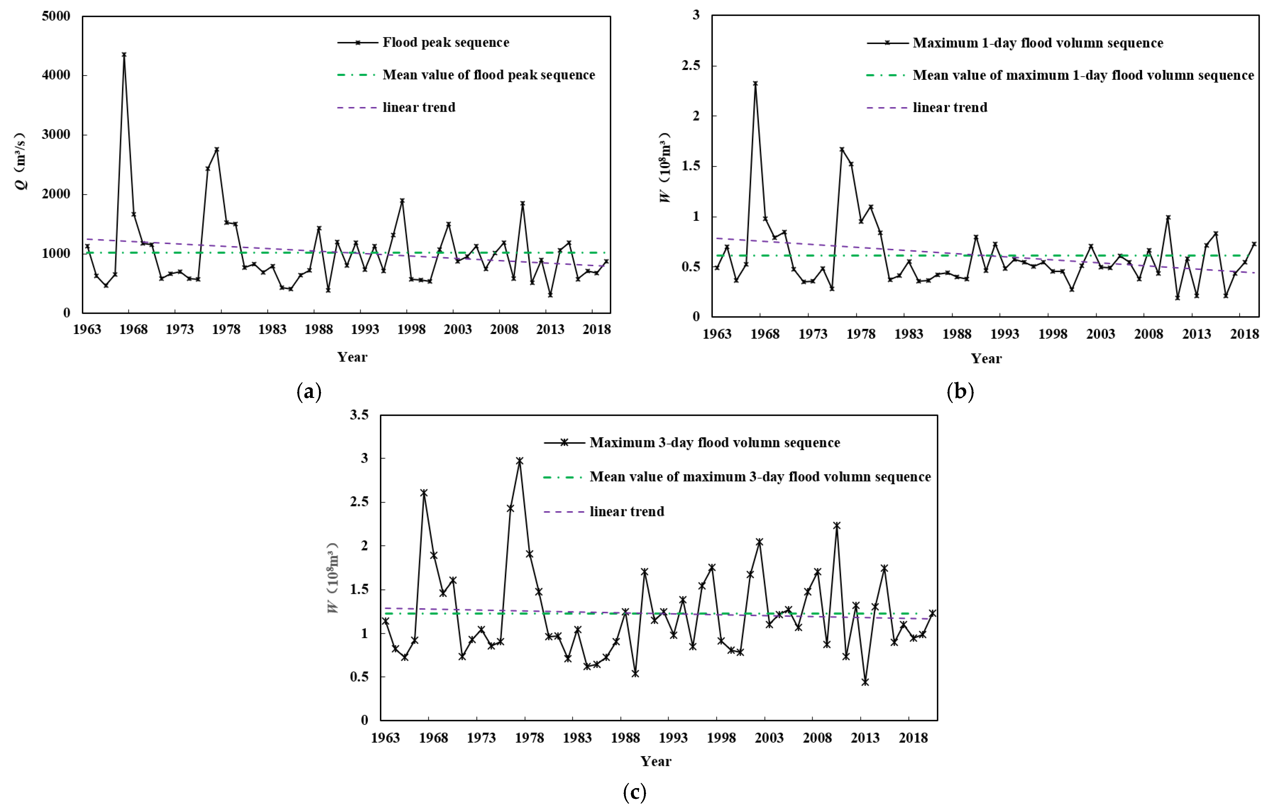
Taking the incoming flood data of Chengbi River Reservoir from 1963 to 2019 as the basis, the mean value of each flood sequence, the sequence value, and the trend line over 57 years were plotted in the same coordinate system; the results are shown in Figure 4. The preliminary and trend diagnoses found that each hydrological series had different degrees of variability, and further quantitative analysis was needed for the years corresponding to the mutation points.

4.1.1. Mutation Diagnosis Results

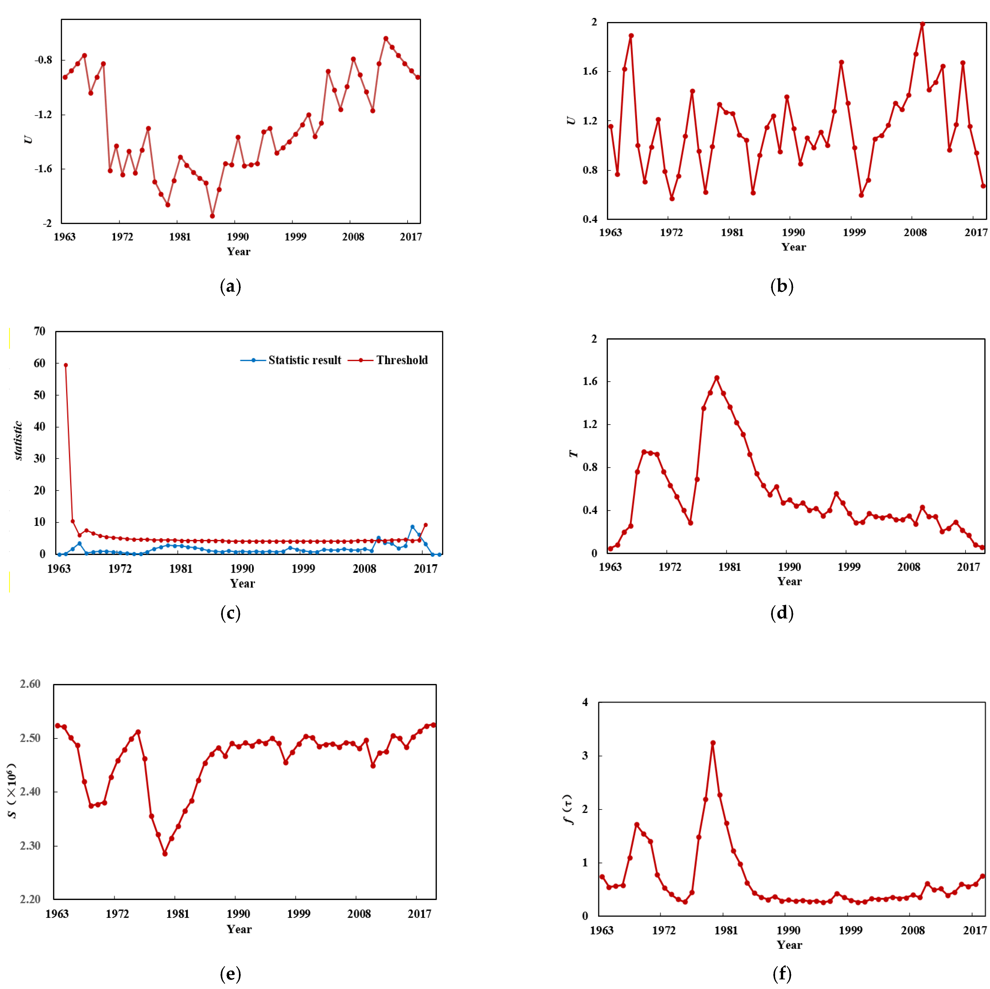
A significance level of $\mathsf{\alpha }=0.05$ was chosen for each diagnostic method in the mutation diagnosis, and the selected methods were the sliding tour test, sliding rank sum test, Brown–Forsythe method, and eight other mutation diagnosis methods listed in Table 1. The results of each method were obtained according to their specific criteria; then, the weights corresponding to each result were determined statistically; finally, the year with the greatest weight was taken as the most likely mutation point. Different indicators were used for each test method in the mutation diagnosis, and the bases for judging the variation point also differed. Comprehensive methods for discriminating types of tests can be roughly grouped into three categories: the first category considers the size of the test indicator value; the second category considers whether the value passes the significance requirements; and the third category considers whether the value exceeds a certain threshold. Taking the annual maximum flood peak sequence as an example, the results of the mutation test for each method are shown in Figure 5.

The mutation years were diagnosed according to the above test criteria, and the combined weights of each mutation year were calculated according to the weight coefficients corresponding to each method in Table 1 so as to determine the most likely year of mutation. A summary of the results of the mutation diagnosis for each flood sequence is shown in

Table 3. Mutation diagnosis results for each sequence.

Mutation Diagnosis Method	Annual Flood Peak Sequence	Annual Maximum 1-Day Flood Volume Sequence	Annual Maximum 3-Day Flood Volume Sequence
Sliding tour test	1986	1980	1996
Sliding rank sum test	2011	1981	1988
Brown–Forsythe method	2010/2015	1979/1980	1966/2015
Sliding t-test method	1979	1980	1979
Ordered clustering method	1979	1980	1979
Lee–Heghinan method	1979	1980	1979
Sliding F-test method	/	1980	1978
Mann–Kendall method	/	1965/1972	/
Year of possible variation	1979	1980	1979
Combined weights	0.3615	0.7977	0.3615

.

As can be seen from Table 2, according to the statistical results for the annual flood peak sequence and annual maximum 3-day flood sequence, the comprehensive weight of 1979 was the largest, and its corresponding weight value was 0.3615; according to the statistical results of the annual maximum 1-day flood sequence, the comprehensive weight of 1980 was the largest, and its corresponding weight value was 0.7977.

4.1.2. Comprehensive Diagnostic Results

The heuristic segmentation algorithm was used for a diagnostic review to determine the final variation points. The results are shown in

Table 4. Diagnosis results of heuristic segmentation algorithm.

Flood Calculation Sequence	Annual Flood Peak Sequence	Annual Maximum 1-Day Flood Volume Sequence	Annual Maximum 3-Day Flood Volume Sequence
$P\left(T_{max}\right)$/splitting point	0.8415/1979	0.9846/1980	0.6907/1979
Diagnosis results	1979	1980	1979

. The splitting points of the annual flood peak and annual maximum 1-day flood sequence were 1979 and 1980, respectively, with $P\left(T_{\max }\right)$ values of 0.8415 and 0.9846, indicating significant sequence variability before and after the cut point; the splitting point of the annual maximum 3-day flood sequence was 1979, with a $P\left(T_{\max }\right)$ value of 0.6907, representing the second most significant sequence variability.

In summary, the annual flood peak, the annual maximum 1-day sequence, and annual maximum 3-day flood sequence of Chengbi River Reservoir all displayed variation, the main form of which was sudden variability. According to our comprehensive diagnosis, the variation point of the annual flood peak sequence and annual maximum 3-day flood sequence was 1979, and that of the annual maximum 1-day flood sequence was 1980.

The climate in the Chengbi River Basin may have been affected by two factors. The first is global warming, with many studies showing that the 1980s was a particularly significant period for the impact of global warming on the climate in China. Our study showed that the flood series in the Chengbi River Basin changed abruptly in 1979, corresponding to the period during which global warming had a significant impact on China’s climate. Another factor that could have affected the climate of the Chengbi River Basin is human activity. Human activity affects the climate by changing the underlying surface. Human activities in the Chengbi River Basin have mainly comprised afforestation and reservoir construction. In the 1980s, China introduced the important reform of the household contract responsibility system in rural areas. The subsequent changes in vegetation cover and increases in land use efficiency may have affected the local climate pattern. The results of our comprehensive diagnosis were consistent with the physical causation analysis, demonstrating that the comprehensive diagnosis identified the most plausible and physically meaningful mutation point.

4.2. Hydrological Frequency Analysis and Design Flood Calculation

Based on the results of the variability diagnosis for the annual flood peak sequence and the annual maximum 1- and 3-day flood volume sequences of Chengbi River Reservoir, we used the simulated annealing algorithm to estimate the parameters of the mixed distribution model for each non-stationarity sequence in order to calculate the design flood process while considering the variability.

4.2.1. Parameter Estimation Results

We estimated the parameters for the mixed distribution model using the simulated annealing algorithm by combining the measured hydrological data of each hydrological station in the Chengbi River Basin. The parameter estimation results of the mixed distribution model for each flood series are shown in

Table 5. Parameter estimation results of mixed distribution method.

Flood Calculation Sequence	α	$\mathit{E}{\mathit{X}}_1$	${\mathit{C}}_{\mathit{v}1}$	${\mathit{C}}_{\mathit{s}1}$	$\mathit{E}{\mathit{X}}_2$	${\mathit{C}}_{\mathit{v}2}$	${\mathit{C}}_{\mathit{s}2}$
Annual flood peak sequence	0.40	1317.94	0.74	2.26	902.34	0.43	1.06
Annual maximum 1-day flood volume sequence	0.41	0.84	0.58	1.85	0.48	0.30	0.85
Annual maximum 1-day flood volume sequence	0.36	1.44	0.59	1.90	1.15	0.37	0.98

, while the parameter results of the traditional P-III distribution without considering the variation are presented in

Table 6. Parameter estimation results of traditional P-III distribution.

Flood Calculation Sequence	$\mathit{EX}$	${\mathit{C}}_{\mathit{v}}$	${\mathit{C}}_{\mathit{s}}$
Annual flood peak sequence	1019.00	0.62	2.26
Annual maximum 1-day flood volume sequence	0.61	0.61	2.21
Annual maximum 1-day flood volume sequence	1.23	0.47	1.64

. The statistical parameters of the sub-series before and after the variation of each flood series were compared, and the mean value $EX$, the coefficient of variation $C_v$, and the bias coefficient $C_s$ changed significantly, which further indicated that traditional P-III distribution with uniform parameters was unsuitable for describing the variation of non-stationary floods.

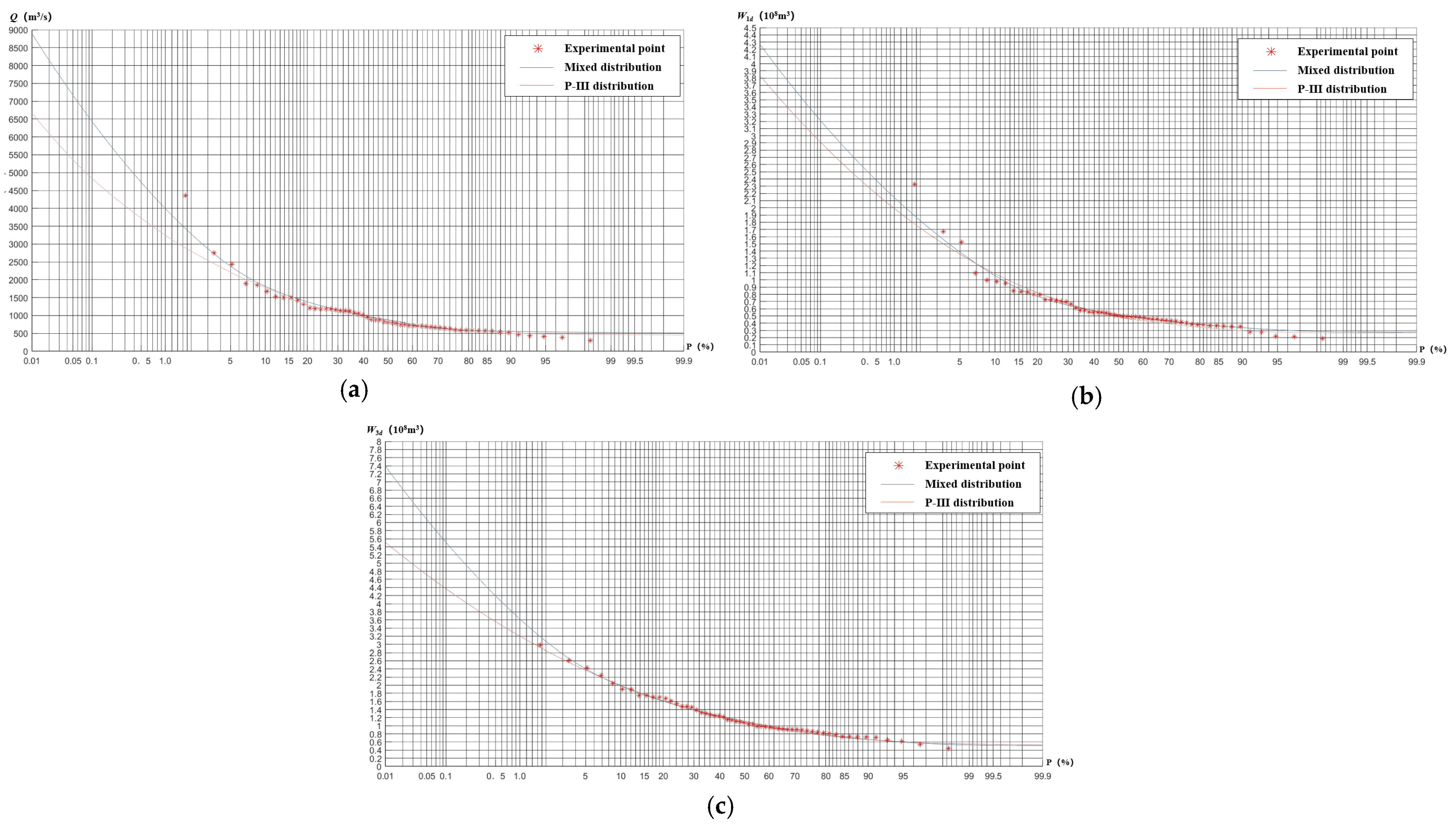
According to the results of the mixed distribution parameter estimation, the expression of the mixed distribution function for each non-stationary flood series could be obtained from Equation (8); thus, the mixed distribution frequency curve could be drawn. In Figure 6, taking the annual flood series as an example, the mixed distribution frequency curve of the annual flood series, the traditional P-III distribution frequency curve, and the empirical frequency point distribution are plotted on the same Hessinger paper. The mixed distribution frequency curve expressed the variation pattern of non-stationary floods more accurately than the traditional P-III distribution frequency curve.

4.2.2. Non-Stationary Design Flood Results

From the frequency curve of the mixed distribution for each flood sequence of Chengbi River Reservoir obtained in Section 4.2.1, the design flood values could be calculated for different standard design flood cases. In order to draw a comparison with adaptive scheduling, the 1000-year and 10,000-year design flood processes in the Chengbi River Reservoir 2013 De-risking Report were taken as typical floods, and the mixed distribution design flood process lines under non-stationarity conditions were deduced based on the annual flood peak sequence, annual maximum 1-day flood sequence, and annual maximum 3-day flood sequence design values. The results are shown in Figure 7.

In Figure 7, under non-stationarity conditions, the mixed distribution design flood process line for 1 in 1000 years and 1 in 10,000 years is located above the typical design flood process line, and the longer the flood recurrence period, the more obvious the increase in the flood process line. As shown in

Table 7. Comparison of design results in terms of annual peak discharge.

Flood Sequence	Once in 1000 Years	Once in 10,000 Years
2013 De-risking	6170	8160
Mixed distribution	6417	8867
Percentage change	4.00	8.66

, the peak of the design flood for Chengbi River Reservoir increased significantly after considering the inconsistent effect of variability, and the increases in the peaks of the 1000-year and 10,000-year design floods were 4.00% and 8.66%, respectively.

In summary, for the same return period, the mixed distribution design flood process for the 1-in-1000-years and 1-in-10,000-years models under non-stationary conditions was less favorable for the reservoir project, and the mixed distribution design flood process line under non-stationary conditions integrated the hydrological series variability and more accurately represented the real variability characteristics of the floods in the study basin under non-stationary conditions. From the perspective of reservoir safety, it would be safer to use the mixed distribution design value under non-stationary conditions as the design criterion in the case of a longer return period.

4.3. Reservoir Flood Control Optimization Scheduling

As shown in Section 4.2, the values for 1000- and 10,000-year floods considering the variability were higher than those of the original design process, and the current scheduling rules for the reservoir would not be able to meet these requirements. Therefore, an optimal scheduling analysis of the mixed distribution design flood was carried out to identify a reservoir scheduling method that could maximize the flood control benefits under the current conditions and fully exploit the reservoir’s flood-regulating capacity under the premise of safeguarding the dam itself, so as to minimize the adverse impacts of variation in the incoming flow due to the changing environment.

4.3.1. Conventional Scheduling Results

The design floods of Chengbi River Reservoir at P = 0.1% and P = 0.01% under non-stationary conditions were routinely scheduled based on initial water levels of 182 and 183 m, and the corresponding scheduling results are shown in Figure 8.

4.3.2. Particle Swarm Optimization Algorithm Scheduling Results

The flood control scheduling model for Chengbi River Reservoir was constructed based on the reservoir optimization scheduling model, and the input of the model was the non-stationary design flood considering variation. The basic idea of the adaptive scheduling approach proposed in this paper was that, depending on the initial water level, the highest flood level of the reservoir should not exceed the design value corresponding to the current frequency during the optimal scheduling process after the variation of the design flood. On this basis, flood control scheduling was carried out by fully exploiting the flood control capacity of the reservoir to ensure the safety of the dam itself while reducing the downstream flood control pressure as far as possible.

Therefore, we took the maximum peak reduction model as an example and used the 1000-year design flood and 10,000-year calibration flood for the simulation, with the maximum water levels set at 187.96 m and 189.29 m. The model was constructed with the minimum sum of squared discharge flow from Chengbi River Reservoir as the objective function and solved by the particle swarm optimization algorithm. The calculation results were a series of flow and water level change processes, and the scheduling results are shown in Figure 9.

4.3.3. Comparative Analysis of Scheduling Results

A comparison of the conventional scheduling results and the scheduling results of the particle swarm optimization algorithm is shown in

Table 8. Comparison of scheduling results (P = 0.1%).

Control Method	Inbound Flood Peak Flow (m3/s)	Maximum Downstream Flow Rate (m3/s)	Peak Reduction Rate (%)	Maximum Water Level after Flood Scheduling (m)
Conventional scheduling	6417	2661	58.5	187.25
Maximum peak reduction	6417	2531	60.6	187.90

and

Table 9. Comparison of scheduling results (P = 0.01%).

Control Method	Inbound Flood Peak Flow (m3/s)	Maximum Downstream Flow Rate (m3/s)	Peak Reduction Rate (%)	Maximum Water Level after Flood Scheduling (m)
Conventional scheduling	8867	3300	62.8	188.71
Maximum peak reduction	8867	3025	65.9	189.26

.

As shown in Table 8, for the 1000-year flood, the maximum water level of the conventional flood control scheduling method was 187.25 m, but this method did not fully exploit the flood control capacity of the reservoir to regulate the incoming flood. Thus, the maximum discharge flow of Chengbi River Reservoir reached 2661 m³/s, with a peak reduction rate of 58.5%. In contrast, although the maximum reservoir level reached 187.90 m during the scheduling process, the flood control optimization method using the maximum peak reduction criterion as the scheduling target fully exploited the flood control reservoir capacity to regulate the incoming floodwater. Thus, the maximum discharge flow of Chengbi River Reservoir was reduced to 2531 m³/s, with a peak reduction rate of 60.6%, and the discharge flow process was smoother, which was conducive to lowering the flood control pressure in the region downstream of the reservoir.

As shown in Table 9, for the 10,000-year flood, the maximum water level of the conventional flood control scheduling method was 188.71 m, but this method did not fully exploit the flood control capacity of the reservoir to regulate the incoming flood. Thus, the maximum discharge flow of Chengbi River Reservoir reached 3300 m³/s, with a peak reduction rate of 62.8%. In contrast, although the maximum reservoir level reached 189.26 m during the scheduling process, the flood control optimization method with the maximum peak reduction criterion as the scheduling target fully exploited the flood control reservoir capacity to regulate the incoming floodwater. Thus, the maximum discharge flow of Chengbi River Reservoir was reduced to 3025 m³/s, with a peak reduction rate of 65.9%, and the discharge flow process was smoother, which was conducive to lowering the flood control pressure in the area downstream of the reservoir. The above analysis proved the effectiveness of the optimal scheduling of reservoir flood control based on the particle swarm optimization algorithm.

5. Discussion

5.1. Similarities and Differences

This study established an adaptive reservoir regulation method integrating hydrological non-stationarity diagnosis, hydrological frequency analysis, design flood calculation, and reservoir flood control and optimization scheduling. We also conducted a case study in Chengbi River Reservoir, aiming at quantitatively analyzing the influence of human activity on floods in the basin in order to reduce the adverse effects of environmental changes on incoming floods by optimizing the scheduling of existing water conservancy projects in the basin. Hence, we proposed a reservoir scheduling scheme that maximized flood control benefits under the current conditions and guaranteed the expected benefits of the reservoir.

The non-stationary flood peaks, etc., calculated while considering mutations, were all higher than those under the original design, leading to an increased risk of flood control downstream, in contrast to the results of other basin studies. Li et al. [40] used four mutation tests, namely, the linear trend correlation coefficient, Mann–Kendall test, sliding t-test, and Pettitt test, to examine the maximum flow from 1950 to 2006 at three hydrological stations in the Iloilo River Basin. The trends and mutations of the series were identified, and the time-series decomposition synthesis method was used to re-fit the design flood series. Chen et al. [41] used the TFPW-MK mutation test and rank sum test to diagnose the variability of the hydrological series at Lanzhou, a representative station in the upper reaches of the Yellow River, and compared the natural runoff series with the measured runoff series to obtain the analysis results. The results showed that the hydrological series of Lanzhou station after the variation point of 1985 presented a significant decreasing trend, and the natural runoff series demonstrated high hydrological variability. For watersheds with significant decreasing trends in their hydrological series, such as the Yellow River [41] and Haihe River [42] basins in northern China, which are water-scarce areas, the main goal of adaptive scheduling should be to increase the use of flood resources through adaptive scheduling when this hydrological variability leads to water shortages. The Chengbi River Reservoir represents a case of hydrological variability leading to increased design flood and increased flood control risk, and so the main objective of adaptive scheduling should be to reduce the flood control risk generated by the hydrological variability. This provides a useful reference for flood-control-oriented basins.

The optimal scheduling results were more effective than the conventional scheduling results, which was consistent with the results of previous studies. Ren et al. [43] used an improved genetic algorithm to optimize flood control scheduling during floods using the Fuziling Reservoir in the Pi River Basin as an example and compared the results with the 2020 flood control scheduling scheme for large reservoirs. The results showed that the design of the original scheduling scheme had certain limitations, and the scheduling results obtained by the optimization algorithm used up as little of the flood control capacity as possible while ensuring the safety of the reservoir and its downstream areas. Conventional scheduling generates scheduling rules based on relevant management experience, providing simplicity and convenience in terms of operation and management, but it does not enable flood resources to be fully exploited. In contrast, optimal scheduling can coordinate the various objectives of reservoir operation, which is crucial for safe operation and the maximization of benefits.

The simulated annealing algorithm is relatively easy to implement, requiring only the generation of new states through random transformations and the computation of objective function values, whereas the particle swarm optimization algorithm requires the tracking of the position and velocity of each particle, which can be much more computationally intensive. Therefore, the simulated annealing algorithm is usually more advantageous when dealing with large-scale optimization problems. Thus, the simulated annealing algorithm was used to solve the mixed distribution model. The PSO algorithm is widely used to solve reservoir optimization and scheduling problems because of its simple structure, limited number of parameters, and low computational requirements.

In previous studies, several scholars have proposed hydrological frequency analysis methods for changing environments. Some scholars have adjusted the reservoir scheduling rules in their study basin and implemented optimal scheduling. Other scholars have proposed new optimal flood control scheduling methods for changing environments, but few have combined these methods. In this study, a system of adaptive reservoir regulation methods integrating hydrological non-stationarity diagnosis, hydrological frequency analysis, design flood calculation, and reservoir flood control optimization scheduling was established.

5.2. Policy Recommendations

Under the influence of climate change and human activities, considering the inconsistency of flood sequences and the influence of reservoir engineering on storage, developing calculation methods for reservoir design floods under a changing environment and deducing reasonable reservoir design flood processes can not only improve our understanding of design flood calculation under variable conditions but also provide data support for flood control planning and the operation scheduling of reservoir engineering. Therefore, hydrologists should carry out research on flood frequency analysis under non-stationary conditions to understand the influence of the changing environment in the basin. Reservoir managers should improve reservoir scheduling schemes to maximize the benefits of reservoirs. In addition, smaller reservoirs could be built on each tributary of the Chengbi River to reduce the hydrological impact when flooding occurs.

5.3. Innovation, Limitations, and Further Research

This study established an adaptive reservoir regulation method integrating hydrological non-stationarity diagnosis, hydrological frequency analysis, design flood calculation, and reservoir flood control optimization scheduling. We aimed to quantitatively analyze the influence of human activities on floods in the Chengbi River Basin, reduce the adverse effects of environmental changes on incoming floods by optimizing the scheduling of existing reservoirs in the basin, and propose a reservoir scheduling scheme that maximized flood control benefits under the current conditions to ensure the expected benefits of reservoirs.

The restricted availability of information limited our research process, and this study could be further improved and expanded in the following directions in future research: Regarding the hydrological frequency analysis, we only performed univariate frequency analysis for non-stationary floods under changing environments; however, flood events are complex and variable, and flood frequency analysis based on multivariate joint distribution could fully elucidate the correlations between each characteristic variable and more accurately describe the evolutionary patterns of flood events. We could use multivariate joint-based flood frequency analysis to understand complex and variable flood events. Regarding reservoir flood control optimization scheduling, we only studied the flood control scheduling of Chengbi River Reservoir. The joint scheduling of upstream and downstream projects combining upstream reservoirs and multiple objectives, such as water supply, flood control, power generation, and irrigation, needs further study.

6. Conclusions

Due to the strong influence of climate change and human activities, the vast majority of reservoirs’ incoming flood sequences no longer meet the consistency assumption. Continuing to adopt the scheduling rules formed during reservoir design often makes the full exploitation of reservoir design functions and benefits difficult and may even increase flood control risks. To this end, we proposed a system of adaptive reservoir regulation and control methods integrating hydrological non-stationarity diagnosis, hydrological frequency analysis, design flood calculation, and reservoir flood control optimization scheduling and applied it to Chengbi River Reservoir. The main conclusions obtained from this study are summarized below.

From the hydrological variability diagnosis results, we concluded that the annual flood peak sequence and the annual maximum 1- and 3-day flood sequences featured mutations. The use of a hydrologic non-stationarity diagnostic system combined with physical causation analysis more accurately identified variability in the flood sequences than a single diagnostic method. The calculation process of the non-stationary flood frequency analysis based on mixed distribution took into account the hydrological conditions under the changing environment, and the non-stationary design flood results obtained considering the point of variability were closer to reality. The particle swarm optimization algorithm scheduling of reservoir flood control under non-stationary conditions allowed the full exploitation of reservoir flood regulation and reduced the downstream flood control pressure.

In future work, we could use multivariate joint-based flood frequency analysis to cope with complex and variable flood events. Furthermore, we could also combine upstream and downstream reservoirs and multiple objectives, such as water supply, flood control, power generation, and irrigation, to conduct joint scheduling studies. Finally, smaller reservoirs could be built on each tributary of the Chengbi River to reduce the hydrological impact when flooding occurs.

References

1. Apurv, T.; Mehrotra, R.; Sharma, A.; Goyal, M.K.; Dutta, S. Impact of climate change on floods in the Brahmaputra basin using CMIP5 decadal predictions. J. Hydrol. 2015, 527, 281–291. [Google Scholar] [CrossRef]
2. Milly, P.C.D.; Wetherald, R.T.; Dunne, K.A.; Delworth, T.L. Increasing risk of great floods in a changing climate. Nature 2002, 415, 514–517. [Google Scholar] [CrossRef] [PubMed]
3. Khaliq, M.N.; Ouarda, T.; Ondo, J.C.; Gachon, P.; Bobée, B. Frequency analysis of a sequence of dependent and/or non-stationary hydro-meteorological observations: A review. J. Hydrol. 2006, 329, 534–552. [Google Scholar] [CrossRef]
4. Vidrio-Sahagún, C.T.; He, J.; Kasiviswanathan, K.S.; Sen, S. Stationary hydrological frequency analysis coupled with uncertainty assessment under nonstationary scenarios. J. Hydrol. 2021, 598, 125725. [Google Scholar] [CrossRef]
5. Pettitt, A.N. A Non-Parametric Approach to the Change-Point Problem. J. R. Stat. Soc. Ser. C Appl. Stat. 1979, 28, 126–135. [Google Scholar] [CrossRef]
6. Inclan, C.; Tiao, G.C. Use of cumulative sums of squares for retrospective detection of changes of variance. J. Am. Stat. Assoc. 1994, 89, 913–923. [Google Scholar]
7. Rodionov, S. A brief overview of the regime shift detection methods. In Large-Scale Disturbances (Regime Shifts) and Recovery in Aquatic Ecosystems: Challenges for Management toward Sustainability; University of Washington: Seattle, WA, USA, 2005; pp. 17–24. [Google Scholar]
8. Villarini, G.; Serinaldi, F.; Smith, J.A.; Krajewski, W.F. On the stationarity of annual flood peaks in the continental United States during the 20th century. Water Resour. Res. 2009, 45, wr007645. [Google Scholar] [CrossRef]
9. Xie, P.; Chen, G.; Lei, H.; Wu, F. Hydrological variability diagnosis system. J. Hydroelectr. 2010, 29, 85–91. (In Chinese) [Google Scholar]
10. Yu, C.; Guo, X. Hydrological Frequency Calculation Method Study of Urban Rivers Runoff under Changing Environment. In Proceedings of the 2nd International Conference on Civil Engineering, Architecture and Building Materials (CEABM 2012), Yantai, China, 25–27 May 2012; pp. 2023–2026. [Google Scholar]
11. Strupczewski, W.G.; Singh, V.P.; Feluch, W. Non-stationary approach to at-site flood frequency modelling I. Maximum likelihood estimation. J. Hydrol. 2001, 248, 123–142. [Google Scholar] [CrossRef]
12. Klein, B.; Meissner, D.; Pinzinger, R.; Lisniak, D. Estimation of the predictive uncertainty of hydrological model simulations and forecasts using copulas. Hydrol. Wasserbewirtsch. 2014, 58, 95–105. [Google Scholar] [CrossRef]
13. Potter, W.D. Upper and lower frequency curves for peak rates of runoff. Eos Trans. Am. Geophys. Union 1958, 39, 100–105. [Google Scholar] [CrossRef]
14. Singh, K.P. A versatile flood frequency methodology. Water Int. 1987, 12, 139–145. [Google Scholar] [CrossRef]
15. Singh, K.; Singh, V. Derivation of bivariate probability density functions with exponential marginals. Stoch. Hydrol. Hydraul. 1991, 5, 55–68. [Google Scholar] [CrossRef]
16. Alila, Y.; Mtiraoui, A. Implications of heterogeneous flood-frequency distributions on traditional stream-discharge prediction techniques. Hydrol. Process. 2002, 16, 1065–1084. [Google Scholar] [CrossRef]
17. Cheng, J.; Song, S. Calculation of frequency parameters based on mixed distribution non-coherent annual runoff series. J. Northwest Agric. For. Univ. Sci. Technol. (Nat. Sci. Ed.) 2010, 38, 229–234. (In Chinese) [Google Scholar]
18. Li, H.Y.; Sun, J.Q.; Zhang, H.B.; Zhang, J.F.; Jung, K.; Kim, J.; Xuan, Y.Q.; Wang, X.J.; Li, F.P. What Large Sample Size Is Sufficient for Hydrologic Frequency Analysis?—A Rational Argument for a 30-Year Hydrologic Sample Size in Water Resources Management. Water 2018, 10, 430. [Google Scholar] [CrossRef] [Green Version]
19. Su, C.; Wang, P.; Yuan, W.; Cheng, C.; Zhang, T.; Yan, D.; Wu, Z. An MILP based optimization model for reservoir flood control operation considering spillway gate scheduling. J. Hydrol. 2022, 613, 128483. [Google Scholar] [CrossRef]
20. Wang, S.; Jiang, Z.; Liu, Y. Dimensionality Reduction Method of Dynamic Programming under Hourly Scale and Its Application in Optimal Scheduling of Reservoir Flood Control. Energies 2022, 15, 676. [Google Scholar] [CrossRef]
21. Foufoula-Georgiou, E.; Kitanidis, P.K. Gradient dynamic programming for stochastic optimal control of multidimensional water resources systems. Water Resour. Res. 1988, 24, 1345–1359. [Google Scholar] [CrossRef] [Green Version]
22. Oliveira, R.; Loucks, D.P. Operating rules for multireservoir systems. Water Resour. Res. 1997, 33, 839–852. [Google Scholar] [CrossRef]
23. Valeriano, O.C.S.; Koike, T.; Yang, K.; Yang, D.W. Optimal Dam Operation during Flood Season Using a Distributed Hydrological Model and a Heuristic Algorithm. J. Hydrol. Eng. 2010, 15, 580–586. [Google Scholar] [CrossRef] [Green Version]
24. Trivedi, M.; Shrivastava, R. Derivation and performance evaluation of optimal operating policies for a reservoir using a novel PSO with elitism and variational parameters. Urban Water J. 2020, 17, 774–784. [Google Scholar] [CrossRef]
25. Ehteram, M.; Othman, F.B.; Yaseen, Z.M.; Afan, H.A.; Allawi, M.F.; Malek, M.B.A.; Ahmed, A.N.; Shahid, S.; Singh, V.P.; El-Shafie, A. Improving the Muskingum Flood Routing Method Using a Hybrid of Particle Swarm Optimization and Bat Algorithm. Water 2018, 10, 807. [Google Scholar] [CrossRef] [Green Version]
26. Mo, C.; Ruan, Y.; Xiao, X.; Lan, H.; Jin, J. Impact of climate change and human activities on the baseflow in a typical karst basin, Southwest China. Ecol. Indic. 2021, 126, 107628. [Google Scholar] [CrossRef]
27. Mo, C.; Tang, P.; Huang, K.; Lei, X.; Lai, S.; Deng, J.; Bao, M.; Sun, G.; Xing, Z. Evolution of Drought Trends under Climate Change Scenarios in Karst Basin. Water 2023, 15, 1934. [Google Scholar] [CrossRef]
28. Mo, C.; Zhu, C.; Ruan, Y.; Lei, X.; Xing, Z.; Sun, G. Study on the Staged Operation of a Multi-Purpose Reservoir in Flood Season and Its Effect Evaluation. Water 2021, 13, 2563. [Google Scholar] [CrossRef]
29. Mo, C.; Cen, W.; Lei, X.; Ban, H.; Ruan, Y.; Lai, S.; Shen, Y.; Xing, Z. Simulation of dam-break flood and risk assessment: A case study of Chengbi River Dam in Baise, China. J. Hydroinform. 2023. [Google Scholar] [CrossRef]
30. Lee, A.F.S.; Heghinian, S.M. A Shift of the Mean Level in a Sequence of Independent Normal Random Variables—A Bayesian Approach—. Technometrics 1977, 19, 503–506. [Google Scholar] [CrossRef]
31. Bao, Q.; Ding, J.; Han, L. Quantifying the effects of human activities and climate variability on runoff changes using variable infiltration capacity model. PLoS ONE 2022, 17, e0272576. [Google Scholar] [CrossRef]
32. Bureau of Hydrology, Yangtze River Water Resources Commission, Ministry of Water Resources. Hydraulic and Hydropower Engineering Design Flood Calculation Specification; Bureau of Hydrology, Yangtze River Water Resources Commission, Ministry of Water Resources: Beijing, China, 2006; Volume SL 44-2006, pp. 99, A95. (In Chinese)
33. Ahmed, E.-S.M.S.; Mays, L.W. Model for determining real-time optimal dam releases during flooding conditions. Nat. Hazards 2012, 65, 1849–1861. [Google Scholar] [CrossRef]
34. Musharavati, F.; Hamouda, A.S.M. Enhanced simulated-annealing-based algorithms and their applications to process planning in reconfigurable manufacturing systems. Adv. Eng. Softw. 2012, 45, 80–90. [Google Scholar] [CrossRef]
35. Lu, S.; Sun, H.; Sun, D.; Guo, M.; Bai, X. Assessment on reservoir flood resources utilization of Ankang Reservoir, China. Resour. Policy 2020, 68, 101745. [Google Scholar] [CrossRef]
36. Zhu, D.; Mei, Y.; Xu, X.; Chen, J.; Ben, Y. Optimal Operation of Complex Flood Control System Composed of Cascade Reservoirs, Navigation-Power Junctions, and Flood Storage Areas. Water 2020, 12, 1883. [Google Scholar] [CrossRef]
37. Kennedy, J.; Eberhart, R. Particle Swarm Optimization. In Proceedings of the Icnn95-international Conference on Neural Networks, Perth, WA, Australia, 27 November–1 December 1995. [Google Scholar]
38. Pan, J.; Wang, H.; Yang, X. A Random Particle Swarm Optimization Algorithm with Application. In Proceedings of the 2nd International Conference on Chemical, Material and Metallurgical Engineering (ICCMME 2012), Kunming, China, 15–16 December 2013; pp. 3940–3944. [Google Scholar]
39. He, Y.; Xu, Q.; Yang, S.; Liao, L. Reservoir flood control operation based on chaotic particle swarm optimization algorithm. Appl. Math. Model. 2014, 38, 4480–4492. [Google Scholar] [CrossRef]
40. Li, X.; Ma, X.; Li, X.; Zhang, W. Method Consideration of Variation Diagnosis and Design Value Calculation of Flood Sequence in Yiluo River Basin, China. Water 2020, 12, 2722. [Google Scholar] [CrossRef]
41. Chen, Y.; Qian, H. Variation in Runoff Series Regimes and the Impacts of Human Activities in the Upper Yellow River Basin. Pol. J. Environ. Stud. 2019, 28, 1071–1082. [Google Scholar] [CrossRef]
42. Du, H.; Xia, J.; Zeng, S.; She, D.; Liu, J. Variations and statistical probability characteristic analysis of extreme precipitation events under climate change in Haihe River Basin, China. Hydrol. Process. 2014, 28, 913–925. [Google Scholar] [CrossRef]
43. Ren, M.; Zhang, Q.; Yang, Y.; Wang, G.; Xu, W.; Zhao, L. Research and Application of Reservoir Flood Control Optimal Operation Based on Improved Genetic Algorithm. Water 2022, 14, 1272. [Google Scholar] [CrossRef]
Figure 1. Schematic diagram of the study area watershed.
Sustainability 15 11530 g001
Figure 2. Water level, reservoir capacity, and discharge flow curves. (a) Water level–reservoir capacity relationship; (b) Water level–discharge flow relationship.
Sustainability 15 11530 g002
Figure 3. Flowchart of this research.
Sustainability 15 11530 g003
Figure 4. The flood sequences and means. (a) Annual flood peak sequence; (b) Annual maximum 1-day flood volume sequence; (c) Annual maximum 3-day flood volume sequence.
Sustainability 15 11530 g004
Figure 5. Diagnostic results of annual flood peak sequence variation. (a) Sliding tour test method; (b) Sliding rank sum test; (c) Brown–Forsythe method; (d) Sliding t-test method; (e) Ordered clustering method; (f) Lee–Heghinan test; (g) Sliding F-test method; (h) Mann–Kendall test.
Sustainability 15 11530 g005aSustainability 15 11530 g005b
Figure 6. Results of fitting the mixed distribution and traditional P-III distribution of non-coherent flood sequences. (a) The annual flood peak flow sequence; (b) The annual maximum 1-day flood volume sequence; (c) The annual maximum 3-day flood volume sequence.
Sustainability 15 11530 g006
Figure 7. Design flood process. (a) P = 0.1%; (b) P = 0.01%.
Sustainability 15 11530 g007
Figure 8. Conventional flood scheduling results. (a) P = 0.1%; (b) P = 0.01%.
Sustainability 15 11530 g008
Figure 9. The scheduling results of the flood particle swarm optimization algorithm. (a) P = 0.1%; (b) P = 0.01%.
Sustainability 15 11530 g009