Article

Morphodiversity as a Tool in Geoconservation: A Case Study in a Mountain Area (Pieniny Mts, Poland)

Department of General Geology and Geotourism, Faculty of Geology, Geophysics and Environmental Protection, AGH University in Krakow, Al. Mickiewicza 30, 30-059 Kraków, Poland
*
Author to whom correspondence should be addressed.
Sustainability 2023, 15(14), 11357; https://doi.org/10.3390/su151411357
Submission received: 19 June 2023 / Revised: 17 July 2023 / Accepted: 19 July 2023 / Published: 21 July 2023

Abstract

:
Verification and delimitation of existing and new surface forms of nature conservation require objective tools that elevate the significance of the conducted evaluations. If our main goal is to preserve biodiversity, it can be ensured through challenging-to-implement practices of human neutrality towards the environment or activities promoting sustainable development that consider the provision of diverse abiotic habitat conditions. For mountainous areas, where the species diversity of plants and animals is strongly linked to the terrain morphology, an analysis of morphodiversity can provide valuable insights. This study examines the morphodiversity of the Pieniny Mts region (southern Poland) in fundamental fields using three mathematical models and various morphometric indicators. The evaluation of existing conservation forms and proposed changes in the analysis were dependent not solely on morphodiversity but also on its autocorrelation. Hot Spot Analysis and Local Indicator of Spatial Association methods were employed, investigating the intensity of spatial clustering of areas with low and high morphodiversity values. Areas with high morphodiversity clustering were defined as justifying legal protection, while those belonging to clusters of fields with low parameter values were considered not to require conservation. Additional insights were gained through the analysis of hot and cold spots, representing fields with high or low morphodiversity surrounded by clusters of fields with contrasting values. The conducted research allowed for the proposing of significant spatial changes for the Pieniny National Park and its adjacent areas to ensure the preservation of high morphodiversity and, consequently, biodiversity.

1. Introduction

The current holistic concept of nature conservation treats the environment as a complex system of interconnected and interacting components of both living and non-living nature [1,2,3,4,5]. Geodiversity [6,7,8,9,10], which solely considers abiotic components such as geological structure, terrain morphology, soil cover, hydrosphere, and climatic variability, determines biological diversity (e.g., [11,12,13,14]). The assessment of geodiversity serves as one of the fundamental tools for effective geoconservation [6,9,10,15,16]. Identifying areas with high variation in abiotic elements of nature is now an important prerequisite for proposing actions aimed at nature protection [12,17,18,19,20,21,22,23].
Geoconservation [15,21,24,25,26,27,28,29,30,31] and the conservation of biotic elements of nature operate today within the framework of sustainable development. The idea, which traces its origins back to the 1960s, aims to ensure the development of societies while guaranteeing similar opportunities for future generations. In the context of geoconservation, the concept of sustainable development emerged through the work of the International Union for Conservation of Nature [32], and subsequently, it was developed by UNESCO [33] and the European Union [34,35]. In Poland, despite the existing rich heritage in nature conservation [36,37,38], attention was relatively late in addressing the issue of conserving non-living natural heritage, towards the end of the 1990s [39,40,41,42,43,44,45,46,47,48]. Currently (July 2023), Poland ranks 12th out of 195 countries signatory to the United Nations “The Sustainable Development Goals” strategy, also known as “Agenda 2030” [49]. Within the “Planet” domain of this strategy, tasks related to the conservation of non-living natural heritage are being implemented [50].
Zwoliński et al. [51] provide a review of methods for assessing geodiversity. Despite the fact that the term “geodiversity” was defined back in the 1990s [24,52,53,54], methods for assessing geodiversity remain subjective. Their subjectivity manifests in the selection of partial criteria assessment and the choice of procedures for assessing overall geodiversity, (e.g., [20,55,56,57,58,59,60,61]). Attempts to objectify these methods are few and involve weighting the partial criteria during the calculation of overall geodiversity using spatial multicriteria analysis (e.g., [62,63,64,65,66]). There have also been attempts to evaluate the quality of partial criteria and overall geodiversity using supervised classification with artificial neural networks [20,67]. These studies demonstrate that non-informative variables and unfavorable data redundancies often appear among the criteria used in geodiversity analyses. The detection of such cases is not based on subjective selection but results from calculations. Therefore, there are potential opportunities for simplifying geodiversity analyses while maintaining their substantive value.
In mountainous areas, characteristics describing morphodiversity play a crucial role in the landscape [20,64,67,68,69]. Undoubtedly, the surface features of the terrain have the greatest influence on how the landscape is perceived by humans. It is the terrain that primarily determines the topoclimatic and habitat variability [4,70] and, therefore, biodiversity [71]. It can be suspected that in mountainous areas, preserving morphological diversity is of crucial importance for the conservation of natural heritage. In the literature on morphodiversity assessments, two dominant research approaches can be identified: objective (qualitative), which assesses the diversity of morphological forms (e.g., [72,73,74,75,76,77,78,79,80,81,82,83,84]); and index-based (quantitative), which defines it based on the analysis of selected topographic attributes (e.g., [85,86,87,88]). Some studies incorporate qualitative analyses into index-based analyses (e.g., [17,20,85,88,89,90,91,92]). Researchers often employ subjective assessment methods and classification schemes in their work, (e.g., [17,20,59,87,92,93]). Despite numerous recommendations to include geodiversity studies in the design procedures of protected areas (e.g., [22,94]), such practices are still not widespread.
This publication is an attempt to simplify the assessment of geodiversity in mountainous areas with high relief dynamics. This assessment was then used to verify existing and delimit new surface forms of nature conservation. The method has a quantitative–qualitative nature and utilizes morphodiversity analysis and three data models based on vector and raster geometry objects, as well as various morphometric indicators. The distinguishing element of the presented analyses compared to other methods and geodiversity studies is the limitation of the assessment solely to relatively easily obtainable data related to the terrain relief, and the dependence of the assessment not on morphodiversity itself but on its autocorrelation. The developed models were tested in the Pieniny Mts region (southern Poland), characterized by significant morphological diversity, a large number of surface forms of nature conservation, and high tourist attractiveness. There have been few studies on geodiversity assessment in the Pieniny Mts region. So far, only the easternmost fragment of the Pieniny Mts has undergone a detailed geodiversity assessment [95]. The analyzed region was also subject to the analysis of geodiversity as part of its research for the entire Western Carpathians [60] and geodiversity of terrain relief as part of research on the Polish part of the Carpathians [89,90]. The developed procedure for assessing surface forms of nature conservation enriches the concept of sustainable development with strong arguments in discussions on nature conservation.

2. Materials and Methods

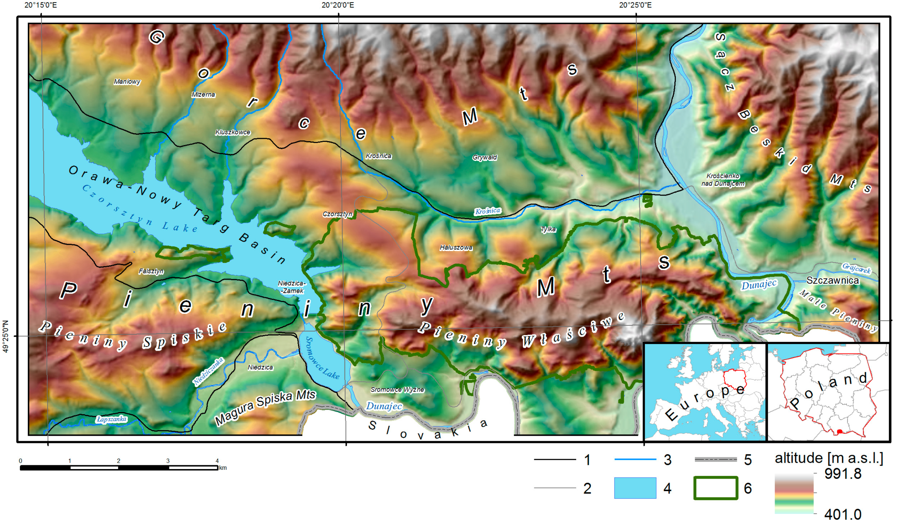
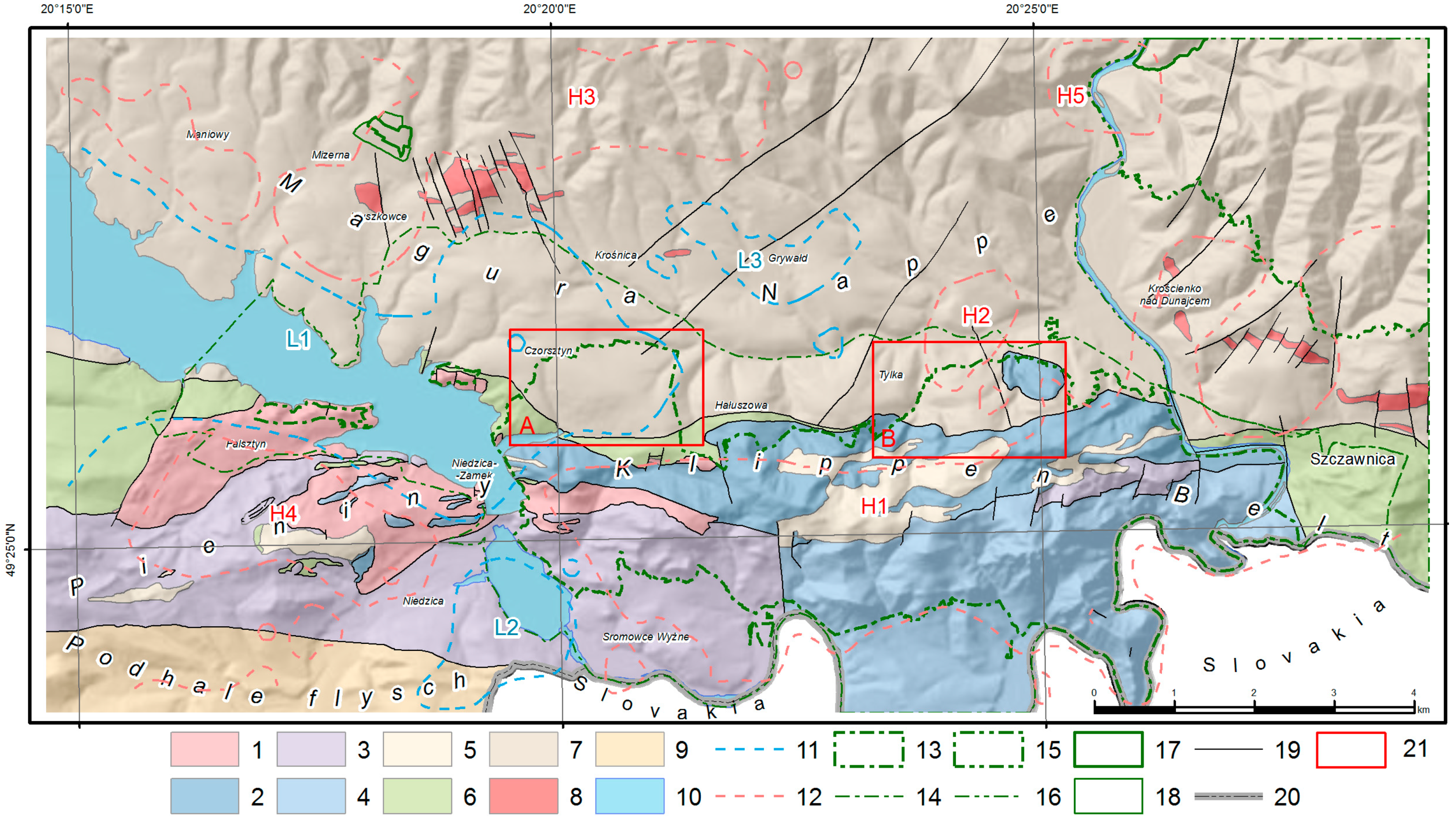
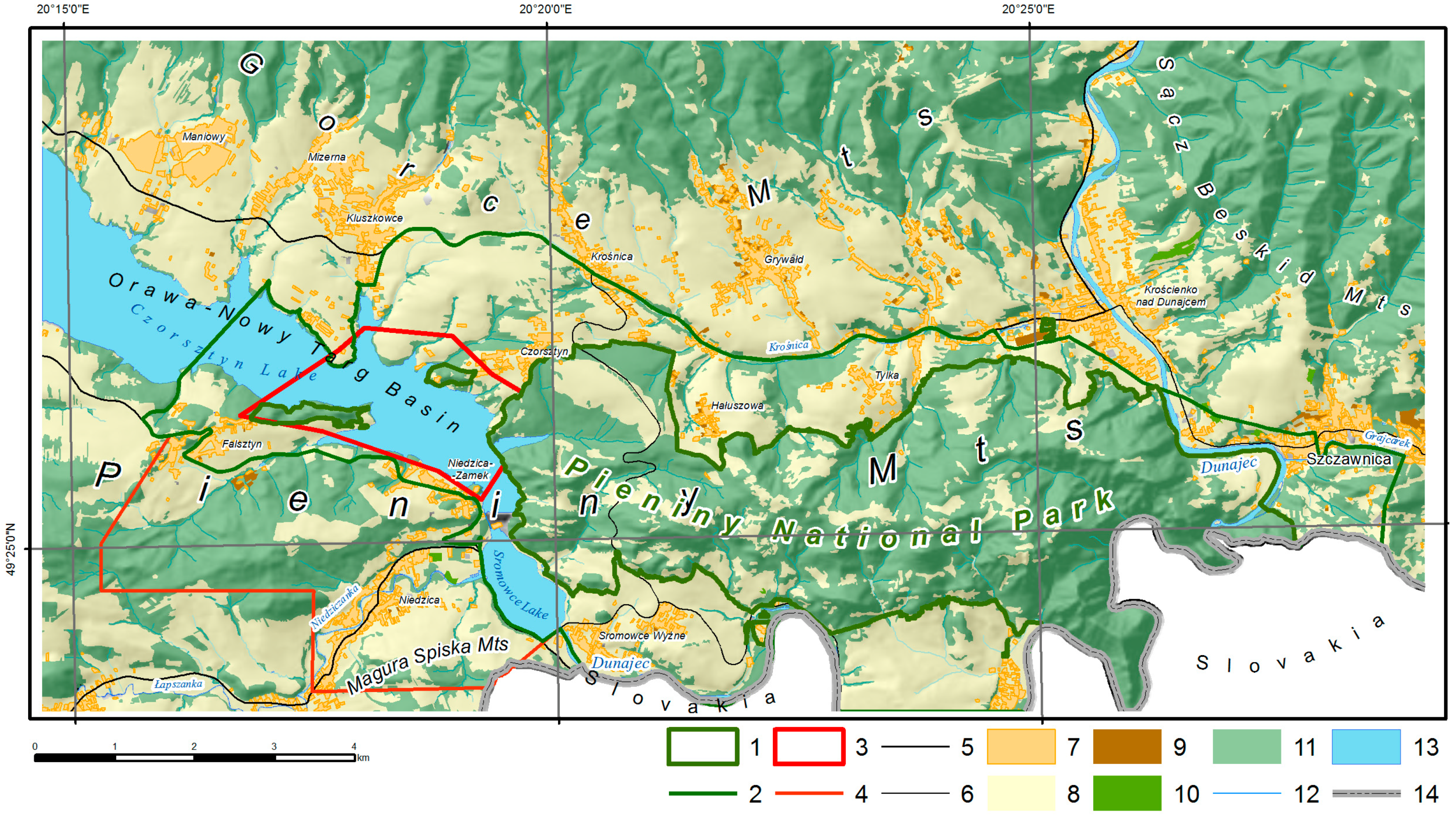
2.1. Geological and Geomorphological Setting

The research area is located in the southern part of Poland in the Małopolskie Voivodeship, partially along the border with Slovakia (Figure 1). The entire research area covered 134.2 km2.
In terms of physical geography, the largest part of the analyzed area (41.8%) is occupied by the Pieniny mountain range (Figure 1) [96]. It is located in the central and southern part of the research area. The Pieniny Mts range is divided into three parts by two antecedent gapes of the Dunajec River: the Pieniny Gap located between Czorsztyn and Szczawnica, partly occupied by the Czorsztyn and Sromowce artificial lakes [97], and the gap between Szczawnica and Krościenko nad Dunajcem. From the west, these are the Pieniny Spiskie, the Pieniny Właściwe (the Central Pieniny Mts), and Małe Pieniny (the Small Pieniny Mts) (mostly outside the analyzed area). Geologically, the Pieniny Mts area is located on the boundary between the Inner Carpathians (to the south) and Outer Carpathians (to the north). It is composed of strongly folded and tectonically disturbed Pieniny Klippen Belt (PKB) formations, formed in the Klippen Basin (Middle Jurassic–Upper Cretaceous) and in the southern part of the Magura Basin (Early Jurassic–Paleogene), covered by the Jarmuta (Upper Cretaceous) and Paleogene formations (Figure 2) [98]. The relief of the Pieniny Mts is the result of complex geological phenomena, with tectonic reduction of the width of the Klippen Basin playing a dominant role. During the Late Cretaceous to the Neogene, the PKB Basin was shortened from its original width of 100–150 km to a few kilometers, and sometimes even a few hundred meters. The outcrops of the Klippen Basin were fractured, crushed, and squeezed, resulting in the formation of positive flower structures [99,100]. Today, the landscape of the Pieniny Mts is characterized by high relief dynamics and the presence of numerous klippen (rocky landforms). Strongly fragmented rock outcrops with varying erosion resistance have shaped the morphology, with steep rocky peaks adjacent to deeply incised river valleys and streams. The cliffs and klippen located in the central and southern part of the Pieniny Właściwe are outcrops of PKB units, while isolated rocky outcrops located in other parts of the PKB are currently interpreted as olistoliths [99].
The smallest part of the analyzed area (approximately 2.2%) is occupied by the Magura Spiska massif (the Spiš Magura Mts), located in its southwestern part. Geologically, it belongs to the Inner Carpathians and is composed of the Podhale Flysch formation, which is part of the Paleogene cover series.
To the north of Krościenko nad Dunajcem, the Dunajec River cuts through the Gorce Mts massif (to the west and center) and the Beskid Sądecki Mts massif (to the east), creating another antecedent gap known as the Small (Beskid) Dunajec River Gap. In the analyzed region, the Gorce Mts mesoregion covers nearly 34% of the area, and the Beskid Sądecki Mts covers approximately 16.4%. Both massifs belong to the Outer Carpathians and are composed of flysch deposits of the Magura Nappe, ranging in age from Early Cretaceous to Neogene. To the west, a narrow strip of the Orawa-Nowy Targ Basin cuts between the Pieniny Mts and Gorce Mts mesoregions. In the studied area, its extent is very close to the shoreline of Czorsztyn Lake. It is a Neogene intramontane tectonic basin filled with Neogene and Quaternary sediments.

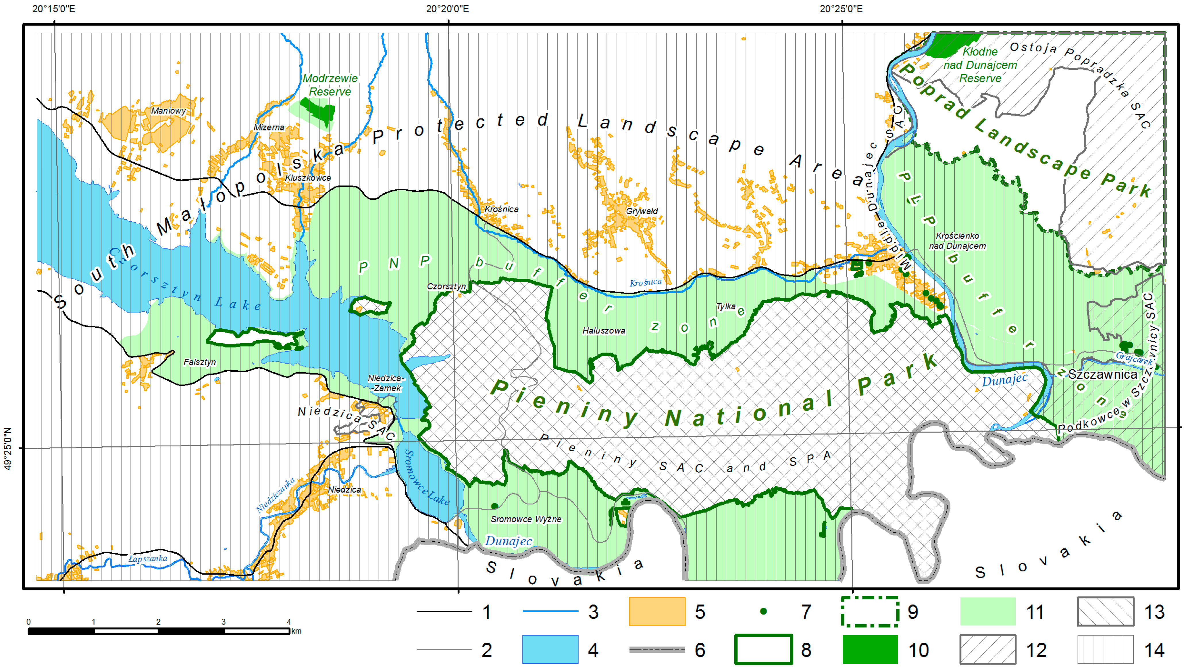
2.2. Nature Conservation

The study area is entirely covered by various forms of nature conservation. Its central part is encompassed by the Pieniny National Park (PNP; Figure 3). It was established in 1932 as the second national park in Poland. It is also the second the smallest national park in Poland. It consists of the main area, which includes the most tourist-attractive part of the Pieniny Mts, as well as ten smaller, isolated enclaves. In total, PNP covers an area of 23.6 km2. The PNP area is also protected as part of the Special Area of Conservation (SAC) network. In addition to PNP, there are four other SAC areas within the analyzed region. The main part of PNP, along with the “Czorsztyn” Castle Hill, is also designated as a Special Protection Area (SPA).
The northeastern part of the analyzed area is encompassed by the Poprad Landscape Park (PLP) along with its buffer zone. There are also two nature reserves in this area—the “Kłodne nad Dunajcem” reserve, established to protect a natural fragment of Carpathian beech forest within the Small Dunajec River Gap, and the “Modrzewie” reserve, which protects Polish larch sites. Almost the entire analyzed area, except for PNP and PLP, is covered by landscape protection as part of the South Małopolska Protected Landscape Area (SMPLA).

2.3. Statistical Zones

The assessment of landscape morphodiversity was based on an artificial analytical grid with hexagonal cells, known as statistical zones. The characteristics of artificial analytical grids were studied by many authors (e.g., [102,103,104]). Parysek [102] demonstrated that grids with hexagonal cells have the highest spatial compactness, allowing for a better illustration of spatial phenomena. The optimal size of the grid cells was estimated using geostatistical autocorrelation analysis. Only landscape features that are represented by continuous regionalized variables could be utilized in this analysis. Absolute elevation and topographic attributes (slope, aspect, plan and profile curvature, and TPI) were used. Suchożerbski [105] reported that statistical zones are homogeneous when their size is 3–5 times smaller than the autocorrelation radius of the variable. Preliminary tests showed that when there are multiple variables, each with a different autocorrelation radius, a compromise must be made when determining block size and consider an intermediate value of the autocorrelation radius. The autocorrelation radii of the analyzed features ranged from several tens of meters (for topographic curvatures) to approximately 3700 m for hypsometry. Due to the high resolution of the DEM, the contour and profile curvatures, which exhibited extremely low autocorrelation radii due to significant anthropogenic terrain modifications, were excluded from this analysis. Finally, a distance of 200 m between the centroids of adjacent statistical zones was adopted as the optimal distance (corresponding to the small diagonal of the hexagons). As a result, the study area was divided into 3876 statistical zones, in which the diversity was assessed based on individual criteria (known as partial criteria), and, subsequently, morphodiversity assessments were performed.

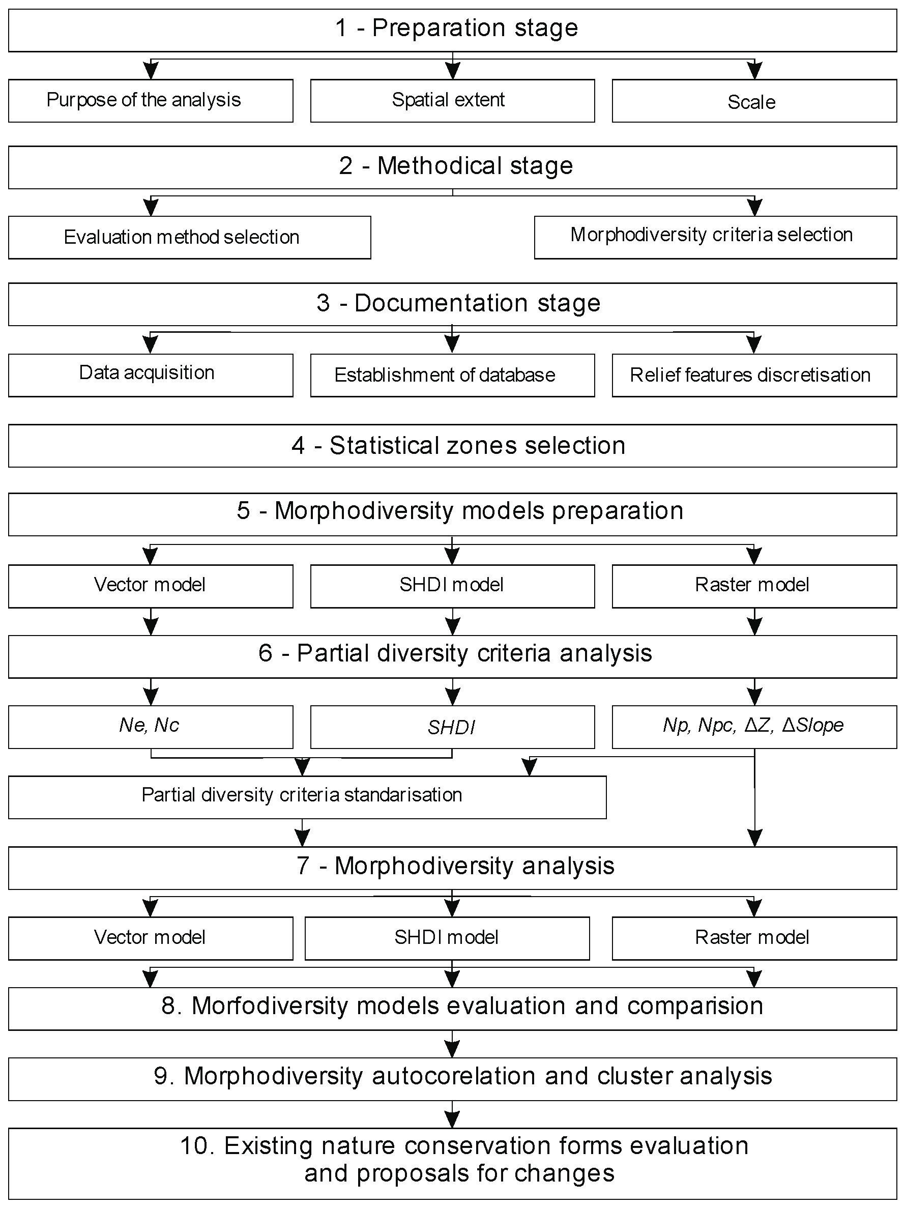
2.4. Outline of the Assessment Methodology

The assessment of morphodiversity in the Pieniny Mts and adjacent areas consisted of ten stages (Figure 4). Firstly, the analysis objectives were defined, the spatial extent was determined, and the detailed scale of the study was chosen (Figure 4, stage 1). These aspects were briefly described in the previous sections of the article. Interval assessment was selected as the evaluation method (Figure 4, stage 2) within the statistical zones (Figure 4, stage 4). The choice was based on its ease of application and the absence of initial assumptions regarding the influence of specific features and criteria on morphodiversity.
In addition to the issues mentioned in the introduction related to the subjectivity of criteria selection and the method of assessing geodiversity, difficulties associated with choosing indicators that represent the intensity of a particular landscape feature should also be considered (e.g., [17,20,70,73,74,106,107,108,109]). Different indices are used for raster data than for vector data. There are indices dedicated to point, linear, and polygonal geometries. Regardless, indices often express slightly different aspects of geodiversity. The most intuitive indices for raster data are the number of pixels of a specific category (Np) and the number of pixel categories (Npc), while for vector data, they are the number of vector objects (Ne) and the number of object categories (Nc). While Npc and Nc express the same qualitative diversity of objects, Np and Ne represent something entirely different. The former measures the area occupied by a given category, while the latter expresses the degree of division of elements into homogeneous patches. A more complex nature is exhibited by the popular Shannon–Weaver index (SHDI) (1) [110]. Although its value depends on the number of categories, unlike simple indices of qualitative diversity (Npc and Nc), it stands out by its sensitivity to the proportions of landscape division into individual categories within specific statistical zones.
S H D I = i = 1 k ( P i · ln P i ) [ ]
i—feature (patch) category; k—number of landscape feature categories; Pi—proportion of a specific category in the landscape (probability of occurrence of a specific category patch in the landscape).

2.5. Relief Features Discretisation

The description of the relief in the Pieniny Mts region was reduced to six typical continuous landscape features (elevation, aspect, slope, planar and vertical curvature, variability of basic landforms—SPIC) and one binary feature (presence of klippen) (Table 1). A significant step in the process was the discretization of continuous landscape features. This was conducted using distribution analysis (Figure 4, stage 3) and the natural breaks method [111]. Some additional comments are needed regarding the discretization of aspect, planar and profile curvature, and basic landforms. The class boundaries for the aspect feature were dependent on the azimuth of the main ridges of the Carpathian arc, which, in this area, is approximately 110° [112]. In flat areas and areas with slight slope, both slope curvatures are landscape features with limited perception, so transformed classes were used in their analysis. The modification involved applying map algebra and calculating spatial intersections with the category of flat areas and areas with slight slope (0–3°). Therefore, the resulting maps, despite being labeled as curvature attributes, are not strictly speaking curvatures themselves but hybrids of them. The feature of basic landforms resulted from the classification of the secondary topographic attribute TPI using the classification proposed by Weiss [113].

2.6. Evaluation Criteria

The defined set of terrain features was described using attributes, referred to as analysis criteria by Sołowiej [114] (Figure 4, stage 2; Table 2). Depending on the type of necessary data, these criteria can be divided into raster criteria (35 criteria) and vector criteria (18 criteria). The first group includes elevation difference (ΔZ), Np, Npc, and slope range (ΔSlope), while the second group includes Ne, Nc, and SHDI.

2.7. Data Acquisition and Preparation

In the documentation stage (Figure 4, stage 3), a database of landscape features and their topographic attributes was constructed. The values were generated using ArcGIS for Desktop software (version 10.8.3) from a 2022 DEM with a resolution of 5 m in the PUWG “1992” coordinate system. To determine the spatial variability of basic morphological forms, the Topographic Position Index (TPI) algorithm was used [113,115]. A circular neighborhood with a radius of 80 m was employed. However, the presence of rocky forms was obtained by digitizing from archival large-scale topographic maps. Hypsometry, aspect, slope, plan and profile curvature, and TPI index values were originally presented in a raster model (Table 2). Only the presence of rocky forms (klippen) was created in a vector model. Due to the high data resolution, minor anthropogenic alterations introduced informational noise into the topographic attribute values. This situation occurred during the modeling of planar and vertical curvatures. In such cases, the Majority Filter method with an eight-pixel neighborhood and a substitution threshold equal to half the number of pixels was applied for generalization [116].

2.8. Morphodiversity Models Preparation

The morphodiversity of the Pieniny Mts area and its adjacent areas was assessed using three alternative evaluation methods: (a) the vector model (2), primarily utilizing data in the vector model and the Ne and Nc indices; (b) the SHDI model (3), mainly utilizing data in the vector model and the SHDI index values; and (c) the raster model (4), utilizing data in the raster model and the Np and Npc indices (Figure 4, stage 5; Table 3). All three models follow an analytical approach, meaning they do not consider relationships between features and rely on defining the final assessment as the sum of partial criteria scores. Certain features of an alternative comprehensive approach, which considers relationships between features, can be found only in the raster model (Figure 5). This is an innovative proposal for evaluating partial criteria based on Np, where partial evaluations depend on the values of other Np indices for the same landscape feature. The method is described in more detail in the Section 2.9. There is some inconsistency in the definition of the models, as raster criteria ΔZ and ΔSlope were used in all three models. This ensured comparability of the results from the three evaluations.

2.9. Partial Diversity Criteria Analysis

Calculations of partial criteria diversity were performed (Figure 4, stage 6; Table 2). The ZonalMetrics toolkit [117] was used to compute entropy index values (1). Due to the use of different indices (Ne, Nc, ΔZ, ΔSlope, SHDI, Np, and Npc), in order to avoid favoring one over the others, the vector diversity models underwent data standardization. Linear data standardization using the min–max method (5) was applied. As a result, sets of partial criteria were obtained with values ranging from 0 to 1.
x i = ( x i x m i n ) x m a x x m i n
xi′—feature value after standardization; xi—feature value before standardization; xmin, xmax—minimum and maximum value of the feature set before standardization
An attempt was made to implement a comprehensive approach based on the raster model (4) (Figure 4), which involved considering the interactions between criteria within the same feature. However, this was not a completely comprehensive approach as it did not take into account interactions between different criteria of different features. In this approach, there was no need to standardize the criteria of the raster model. The calculation procedure was as follows: assuming k as the number of discrete categories describing the diversity of raster continuous landscape features, each such feature was described by a set of indices (e.g., Np1Aspect, Np2Aspect, …, NpkAspect) (Table 2). The starting point of the considerations was the observation that the lowest partial diversity of a criterion based on Np occurs when the observed Np value of a particular category is zero within the statistical zone (Figure 5A), or when the selected category of a given feature covers the entire base field (Figure 5B). On the other hand, the highest diversity occurs when the proportions of the area occupied by pixels of each category are equal within the statistical zone (Figure 5C). This means that the diversity of criteria based on Np should be influenced by the coverage proportions of the statistical zone by individual pixel categories of the same landscape feature. The partial diversity of any Npi criterion (i = 1, …, k) should increase until the coverage by pixels of that category reaches 1/k × a, where a represents the total number of pixels in the statistical zone (see Figure 5C), and then it should start to decrease to zero. For example, for a five-level diversity assessment and a number of categories of any landscape feature k = 6, the diversity of each Np index can be graphically presented using the relationship shown in Figure 6.
In the next stage of the research, morphodiversity calculations were performed using three defined models (Table 3; Figure 4, stage 7). Bonitation into five grades of morphodiversity—very low (1), low (2), middle (3), high (4), and very high (5)—was conducted using the equal interval method. The evaluations of morphodiversity were subjected to initial visual assessment, and then compared with each other using the Spearman rank correlation coefficient and the coincidence index of assessments (morphodiversity grades) (Figure 4, stage 8).

2.10. Clustering of Morphodiversity Assessments

The elimination of informational noise that appeared on the morphodiversity assessment cartograms hindered their interpretation. To eliminate it, clustering was performed. This required conducting a Global Spatial Autocorrelation Analysis of morphodiversity, which allowed for the assessment of the strength and distance at which the clustering phenomenon is most pronounced. Incremental autocorrelation analysis was used for this purpose (Figure 4, stage 9). It reflects the intensity of spatial clustering of statistical zones. The analysis uses statistically significant maximum z-score values—the standardized global Moran’s I statistic [118], which measures spatial autocorrelation and is calculated for different distances between the statistical zones. The distance at which it reaches its maximum (maximum autocorrelation) indicates the distance at which spatial processes favoring object grouping are most pronounced.
To locate clusters of objects with high and low values of the analyzed parameter, autocorrelation analysis of morphodiversity was conducted using the Hot Spot Analysis method. It utilizes the Getis-Ord Gi* statistic [118]. The adopted method allowed for classifying fields into two types of clusters—high or low morphodiversity—with high levels of significance (99%, 95%, and 90%). The validity of protected area boundaries was verified based on the level of probability with which hexagons belonged to high morphodiversity clusters (Figure 4, stage 10). Clusters of statistical zones characterized by high values of the analyzed parameter and located outside of the PNP and PLP areas were considered for potential expansion of protected zones. Objects that belonged to low morphodiversity clusters with high probability (≥90%) and fields with uncertain assessment (NS) were deemed not eligible for area-based protection. The principle was applied where each field was analyzed in the context of neighboring objects located within a distance of less than 1000 m (five statistical zones).

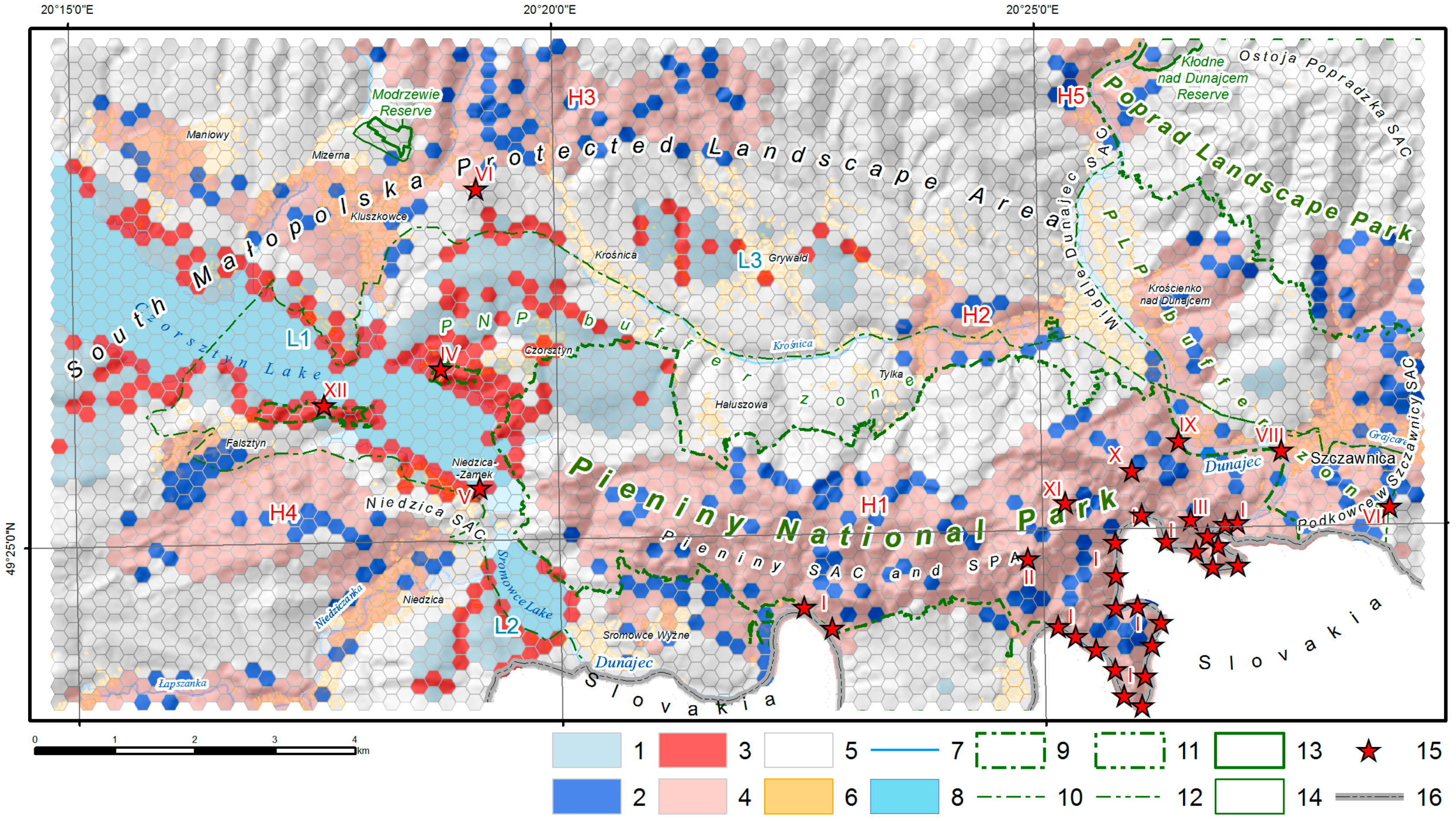
2.11. Searching for Hot and Low Spots

Within clusters of high and low levels of the analyzed parameter, local anomalies often occur. Their occurrence was utilized for further verification of the suitability of legal protection for specific areas. The Local Indicator of Spatial Association (LISA) analysis [119] was applied, which examines the local autocorrelation of morphodiversity to determine the similarity of each spatial object to its local neighbors. The tool utilizes local Moran’s I statistics, z-score values, and the probability of the occurrence of the clustering phenomenon by chance. The analysis allowed for the identification (at a significance level of 0.05) of statistical zones with a high level of morphodiversity surrounded by objects with high morphodiversity values (HH); fields with a low parameter level surrounded by objects with low morphodiversity values (LL); fields with hot spot characteristics, i.e., objects with high morphodiversity values surrounded by objects with low morphodiversity values (HL); and fields with cold spot characteristics, i.e., objects with low morphodiversity values surrounded by objects with high morphodiversity values (LH). Statistical zones with low values of the analyzed parameter located within clusters of high diversity were considered unfavorable for inclusion in planned area-based nature conservation forms. Hexagons with high levels of morphodiversity located within clusters of low diversity were deemed favorable for inclusion in area-based or point-based nature conservation projects.

3. Results

3.1. Morphodiversity Evaluation

The landscape of the Pieniny Mts region is characterized by a high level of morphodiversity. The distributions of ratings from the three alternative morphodiversity models are similar, and all of them exhibit negative skewness (Figure 7, Figure 8 and Figure 9). On average, over half of the statistical zones received ratings of high or very high morphodiversity. At this stage of the research, cautiously speaking, the raster model can be considered the most optimistic as it classified the highest number of fields into the high and very high morphodiversity categories.
The Spearman coefficients, when comparing the rank correlations of ratings, were statistically significant and similar to each other. They ranged from 0.73 to 0.77 (Table 4). The analysis also revealed a high level of coincidence in the ratings calculated through all three models. The lowest coincidence rate (66.9%) was observed when comparing the modeling effects between the raster and SHDI models, while the highest (69.8%) was found when comparing the ratings of the vector and raster models.
Spatial variability of morphodiversity ratings exhibits a significant level of information noise (Figure 7, Figure 8 and Figure 9), but even at the preliminary analysis stage of the cartograms, certain regularities can be identified. The most important nature conservation area in this region, the PNP, is characterized by a relatively higher level of morphodiversity and less variation in ratings compared to neighboring areas. It also contains the highest number of fields with a very high level of morphodiversity. These phenomena are best represented in the cartograms generated for vector models (Figure 7 and Figure 8). The cartogram produced for the raster model presents a slightly different picture (Figure 9). Although the entire PNP area also exhibits a high level of morphodiversity, isolated statistical zones with a very high level of relief variation appear in similar proportions in the areas of the Beskid Sądecki Mts and the Gorce Mts. The observed information noise suggests the need for clustering of statistical zones.

3.2. Autocorrelation of Morphodiversity

The analysis confirmed that morphodiversity ratings exhibit varying spatial autocorrelation (Figure 10). The SHDI model shows the highest intensity of object clustering, and the processes leading to this clustering extend up to approximately 3 km, which is three times further than in the case of the raster model. These parameters are intermediate for the vector model. Statistical zones that are closer or farther apart than this distance exhibit a greater random component in the overall variation of morphodiversity. For further investigations, the most pessimistic model was selected, which exhibits the weakest tendency to cluster fields with high or low ratings, namely, the raster model. The verification of existing nature forms using the Hot Spot Analysis, LISA methodology, and models with stronger autocorrelation (and longer distances at which autocorrelation reaches its maximum) would be impossible due to overly optimistic classification of objects, resulting in bimodal cartograms with extensive clusters of fields with high and low levels of morphodiversity.

3.3. Verification of Existing Protected Area Boundaries

Hot Spot Analysis of the raster model of morphodiversity revealed the presence of several larger and smaller clusters characterized by low or high levels of morphodiversity within the Pieniny Mts region and its vicinity (Figure 11). The central parts of these clusters consist of core areas, whose membership to the respective zones was confirmed at a significance level of 0.01 (99% probability). The outer parts of the clusters surround statistical zones classified at a lower level of significance (0.05 and 0.1). Between the clusters of fields with high and low levels of morphodiversity, there are zones with fields exhibiting variable terrain diversity that could not be classified into any cluster with a probability exceeding 90%. There are more clusters with a high level of morphodiversity than those with a low level.
The largest cluster of fields with high morphodiversity has a latitudinal elongation and encompasses a part of PNP located between Sromowce Wyżne and Szczawnica (Figure 11(H1)). Only the northern and western parts of PNP are not included in this cluster. With the exception of PNP enclaves, almost all of the most spectacular natural features of this region are located within this cluster. In the eastern part, this cluster extends beyond the boundaries of PNP and continues in the Krościenko nad Dunajcem area and in the southwestern part of the Beskid Sądecki Mts, where it includes a part of PLP and its surroundings. A small fragment of the cluster extends beyond the park’s boundaries, also in its southwestern part, near Sromowce Wyżne. The PNP buffer zone, except for three fragments located northeast of Sromowce Wyżne (H1), northeast of the village of Tylka (H2), and in the vicinity of Falsztyn (H4), has been classified as a cluster of statistical zones with low morphodiversity or which could not be classified with a probability greater than 90%. Clusters of fields with high morphodiversity also occur within the SMPLA protected landscape area, partially within PLP. They include areas located along the southern edge of the Gorce Mts (H3), within the Pieniny Spiskie between Falsztyn and Niedzica (H4), and within the southern part of the Small Dunajec River Gap north of Krościenko nad Dunajcem (H5). Their outer parts, which have been classified into clusters at a lower level of significance, are often wider. This indicates a lower relief dynamic in these areas compared to the main cluster covering PNP. The largest cluster of statistical zones with low morphodiversity occurs within the Orawa-Nowy Targ Basin (Figure 11(L1)). Smaller clusters of such fields also occur within the northern foreland of the Magura Spiska Mts (L2) and in the Grywałd area (L3).
LISA confirmed a high similarity in the results of morphodiversity modeling conducted using the three proposed models (Figure 12). Within almost all analyzed nature conservation forms, the variability structures of clusters with high (HH) and low (LL) levels of morphodiversity, as well as cold (LH) and hot (HL) spots, were very similar. Therefore, the differences between them can be attributed solely to the nature of the indicators used. The areas of PNP, SPA, and SAC largely overlap (Figure 3); hence, their cluster structures are similar to each other. Morphodiversity modeling using the SHDI model consistently resulted in a higher proportion of statistical zones classified into the high parameter cluster (HH) and lower numbers of cold spots (LH) compared to the alternative models. Larger and more restrictive nature conservation forms such as PNP and PLP have smaller proportions of NS fields compared to other areas. It can also be observed that within PNP and PLP, compared to their buffer zones, there is a higher proportion of fields belonging to clusters with a high level of morphodiversity (HH) and a lower proportion of fields belonging to clusters with a low level of morphodiversity (LL). This indicates a favorable design of their boundaries in terms of morphodiversity. Within PLP and its buffer zone, as well as within reserves, no fields with a high level of morphodiversity were found within clusters of fields with a low parameter level (HL).

4. Discussion

The analysis of cartograms, taking into account morphodiversity analysis, geological structure coherence, and land use type, confirms that the boundaries of PNP have generally been designed with high precision (Figure 13). Over 53% of the park’s area is occupied by statistical zones belonging to the cluster with a high level of morphodiversity (H1), and over 5% of fields (mainly within PNP enclaves) consist of objects with a high level of morphodiversity located within the cluster with a low level of this parameter (HL). Within PNP, like in any structure of this type, there are also statistical zones with a low level of morphodiversity (LH). They occur throughout the park’s area and collectively occupy about 17% of its surface. The spatial distribution of these fields is similar to random, making it difficult to use them in reasoning about the correctness of the park’s boundary design. Only the presence of a cluster of fields with a low parameter value located in the western part of PNP (L1), as well as fields with uncertain class membership located in the northern part of the park, which together cover about 1/4 of its area, may raise some concerns.
In areas of low or uncertain morphodiversity located between Czorsztyn and Hałuszowa, as well as between Tylka and Krościenko nad Dunajcem, the boundary of PNP turns north, forming two characteristic peninsulas (Figure 13). When entering them from the south, we cross the northern edge fault and move from the PKB area to the Magura unit of the Outer Carpathians (Figure 2(A,B)). It is composed of flysch formations, represented here by sandstones and shales. The change in geological structure is accompanied by a change in the terrain relief. There are no steep peaks characteristic of PKB, nor meandering valleys deeply incised into their substrate. The inclusion of these areas within the park boundaries was determined by the presence of extensive meadows and pastures (see Figure 14) [120] with protected plants and habitats of rare invertebrates, mainly insects [121]. Despite their low or uncertain morphodiversity, excluding these areas from the PNP boundaries would not be desirable.
Around the boundaries of the park, within its buffer zone, there are several areas that represent potential opportunities for expanding its boundaries. Within the outer parts of clusters with low morphodiversity, we often encounter hot spots (HL) (Figure 13). This is particularly evident around the edges of Czorsztyn and Sromowce Lakes. These are highly attractive tourist regions, characterized by strips of sometimes steep hills of relatively low relative height and frequent rocky formations. The most attractive areas, such as those located west of Czorsztyn or between Falsztyn and Niedzica, are currently enclaves of the PNP. Of course, the observed hot spots (HL) effect may partly be due to the radical change in morphodiversity occurring at the boundary of the cluster of statistical zones with low parameter level encompassing Czorsztyn Lake (L1) and the land. In reality, however, the high morphodiversity of these areas is influenced by natural conditions. A testament to this is the complex shoreline of Czorsztyn Lake, with numerous bays and promontories (Figure 1). Noteworthy is the different formation of the opposite shores of Czorsztyn Lake. The northeast shore is mainly composed of hard, erosion-resistant limestone (Figure 2) [101]. The surrounding slopes exhibit complex morphology, high steepness, significant variations in exposure, inclinations, and curvature. To the east of the castle hill in Czorsztyn (Figure 13(IV)), extensive landslides have formed in places where less erosion-resistant rocks occur. The southwestern shore of the lake looks different. Here, sandstones, mudstones, shales, and Upper Cretaceous marls belonging to the Czorsztyn unit, which are less erosion-resistant, play a leading role in the geological structure. Consequently, the lake shores and surrounding slopes are not as steep, and rocky formations occur only in the areas of Niedzica Castle (Figure 13(V)) and Zielone Skałki (XII). Among other areas located in the vicinity of the PNP, it is also worth mentioning the cluster of morphodiverse fields located northeast of the village of Tylka (Figure 13(H2)). This is an enclave of Pieniny Mts limestone within the Magura unit of the Outer Carpathians (Figure 2), and morphologically, it largely belongs to the Gorce Mts [96]. Due to the developed rural development in this area (see Figure 14), it should not be considered for protection within the PNP.
Only about 16% of the surveyed area of the PLP showed membership in the cluster of statistical zones with a high level of morphodiversity. This includes the southern part of Small Dunajec River Gap (Figure 13(H5)) and a fragment of the Beskid Sądecki Mts located north of Szczawnica (eastern part of H1). The PLP area, analyzed in its entirety, belongs to the Outer Carpathians and is built of the flysch formations of the Magura Nappe (Figure 2). In the southern part, these formations are crosscut by bands of Neogene intrusions known as the Pieniny Andesite Line. The discussed area is located in the peripheral part of the PLP, whose main focus of protection is the landscape of the Poprad River valley (outside the surveyed area). Therefore, the conducted analyses do not determine the necessity of including it within the PLP protection. Considering the radical change in the geological structure that occurs after crossing the Dunajec River, when transitioning from Pieniny Mts to Beskid Sądecki Mts, as well as the urban agglomeration of Szczawnica that separates these areas, it also seems unreasonable to include the morphodiverse eastern part of cluster H1 in the PNP.
The extensive and morphodiverse cluster of statistical zones located within the southern edge of the Gorce Mts is densely populated and predominantly used for agricultural purposes in the areas surrounding the villages of Maniowy, Mizerna, and Kluszkowce (Figure 1). This makes it impractical to subject it to strict forms of nature protection. It appears that including it within the landscape protection of the SMPLA is the optimal solution.
The functioning floristic reserve “Modrzewie”, which covers a portion of the surveyed area, has been classified as an NS type during the analysis of morphodiversity. Its establishment is associated with high biotic values. The same applies to the forest reserve “Kłodne nad Dunajcem” located within the southern section of the morphologically diverse Small Dunajec River Gap. The conducted analyses do not provide grounds for verifying the boundaries of these objects.
The area located west and southwest of the PNP has the greatest potential for the revaluation of existing nature conservation forms. There exists a large cluster of statistical zones with a high level of morphodiversity, as well as several extensive smaller objects classified as hot spots. It is proposed to extend the boundaries of the PNP westward to include a portion of the Czorsztyn Lake and the adjacent morphodiverse areas along its shores (Figure 14). The boundary would run along the line from Falsztyn to Kluszkowce. As part of the delimitation of the new boundaries, two enclaves would be included within the consolidated part of the PNP—Zamkowa Mt, with the castle in Czorsztyn (see Figure 11(IV)), and Zielone Skałki (see Figure 11(XII)). Additionally, the castle hill with the “Dunajec” castle in Niedzica would also be encompassed within the park’s boundaries (see Figure 11(V)). The reasons supporting the inclusion of this area into the PNP are its high morphodiversity, geological coherence, numerous rocky formations, high biodiversity as reported in works by Dąbrowski [121] and Kajcer [122], and its high tourism-attractiveness. Due to the proximity to the Czorsztyn Lake and the recent development of tourist infrastructure, this area is particularly vulnerable to anthropogenic pressure. The high biodiversity of the areas surrounding the Czorsztyn and Sromowce lakes would also require the simultaneous expansion of the boundaries of existing SAC and SPA sites. Furthermore, it is proposed to extend the buffer zone of the PNP to include highly morphodiverse but partially densely inhabited areas located between Falsztyn and Niedzica (Figure 14).
As mentioned in the introduction, the preservation of abiotic landscape diversity is one of the fundamental goals of geoconservation [24,123]. Therefore, one of the natural ways to utilize geodiversity assessments is to use them for the evaluation of existing protected areas, the formulation of conservation strategies, and the delimitation of new areas [19,25,61,73,91,124]. Studies addressing this topic strive to connect discrete assessments of geodiversity in statistical zones with the boundaries of existing protected areas or use these assessments to design the boundaries of new protected areas (e.g., [17,20,61,63,64,109,125,126,127]). Delimiting new forms of nature conservation is sometimes associated with assessments of additional criteria, such as biodiversity analyses, land use, and others, e.g., [17,20,127]. Such an approach works well in small-scale studies, where statistical zones typically have large sizes. However, in large- and medium-scale studies, where assessment units are usually much smaller, the assessments are challenging due to the presence of informational noise. The proposed method allows for replacing mosaic-like distributions of geodiversity assessments with clusters of fields with high or low diversity, which are created with a high probability. The resulting cartograms are clear and easy to interpret.

5. Conclusions

The modeling of geodiversity using three defined models—vector-based (primarily based on Ne and Nc indicators, as well as SHDI based on entropy), as well as raster-based (primarily based on Np and Npc indicators)—yielded very similar results. Random factors and the properties of the used indicators collectively accounted for no more than 27% of the variability in the evaluated assessments. The evaluations of the raster-based and SHDI models differed the most from each other, while the vector-based (primarily based on Ne and Nc indicators) and raster-based models produced the most similar results. The evaluation results themselves do not warrant recommending any of the proposed models as significantly better than the others. Only the lower required effort may favor recommending the use of the SHDI model for analysis.
Analyses of landscape feature diversity based on raster data and Np indicators require a special rating procedure that takes into account the proportions of the surface area occupied by pixels of each category within the entire statistical zone. The application of this procedure allows, to some extent, the replacement of the employed simplified analytical approach with a more comprehensive method that better captures the complex interactions occurring between environmental features. Unfortunately, the applied method should be understood as incomplete since it only considers interactions between certain criteria of the same landscape feature and does not account for interactions between criteria of different features.
Due to the observed informational noise, evaluations of existing nature conservation areas and proposals for changes based on unprocessed models of morphodiversity would be challenging to implement. A solution to this problem is to depend not only on morphodiversity itself but also on its autocorrelation, which enables clustering. Clustering of morphodiversity allows for the assessment of the fit between the boundaries of protected areas and the assumed high probability. The method also enables the acquisition of information about morphodiverse areas located outside protected areas and within clusters of low or uncertain morphodiversity fields. Such areas can be qualified for detailed studies aimed at their protection. Incremental autocorrelation analysis showed that the defined models of morphodiversity reflect to varying degrees the influence of spatial phenomena on the grouping of cells in the analytical grid. This applies to both the spatial range in which clustering was most pronounced and the strength of this relationship. Autocorrelation of morphodiversity was most strongly reflected in the SHDI model and least strongly in the raster model. This may indicate that the SHDI model better captures the morphodiversity of mountainous areas than other methods. Confirmation of this hypothesis will require further research.
Calculations of morphodiversity using the raster model resulted in a relatively higher number of higher morphodiversity ratings compared to the alternative models considered. However, LISA analysis revealed that it was the SHDI model that caused a greater number of fields to be classified into clusters of high morphodiversity levels. Further research is needed to explain this phenomenon.
During LISA analysis, in areas where water reservoirs meet land or flat areas adjoin morphological edges, there is often a classification of statistical zones into the group of hot spot fields (HL). Such classification results may reflect real morphological contrasts, but they can also be the result of methodological imperfections. Classifications of such fields should be treated with a greater degree of skepticism.
The greatest strength of the presented method for assessing and delimiting nature conservation areas in mountain regions is its applicability to any set of criteria and any adopted geodiversity model. The evaluation of nature conservation boundaries in the Pieniny Mts region was conducted assuming that their course was mainly determined by the terrain morphology. However, this assumption may not hold true for all protected areas. Expanding the presented method to include selected biotic criteria (or others) will significantly enhance its significance.
One inconvenience of the presented method is its strong dependence on defining the scale of analysis. It is determined by the smallest distance at which spatial processes favoring the clustering of statistical zones operate most strongly or clearly. Determining this distance requires the conducting of Spatial Incremental Autocorrelation Analysis. In maps of score distributions, where autocorrelation is pronounced and extends over large distances, an unfavorable phenomenon of binary classification of statistical zones occurs. The resulting Hot Spot Analysis maps contain only two large clusters of fields with low and high geodiversity, lacking fields of the NS type, and subtle details of cluster boundaries are blurred. Interpreting such maps is very difficult and sometimes impossible. Paradoxically, for clustering statistical zones for the purpose of evaluation or delimitation of protected areas, models with lower levels of score autocorrelation and shorter scales of analysis are better suited. Generated classifications then consist of many smaller clusters of fields with high and low values of the analyzed parameter, separated by wide zones of NS fields. Such maps contain many interesting details that aid in the conducted interpretations.
The Pieniny Mts region is characterized by a high level of morphodiversity and a significant concentration of diverse surface nature conservation areas. The high morphodiversity of the areas surrounding the Czorsztyn Lake and within the Pieniny Spiskie Mts, along with the richness of insect habitats, particularly butterflies and waterfowl, as well as the rapid development of tourism in this region, provide grounds for considering the inclusion of these areas within the Pieniny National Park.
The protection of biodiversity on our planet is one of the fundamental goals of sustainable development. The analysis of morphodiversity, and particularly its autocorrelation, can be recommended for mountainous areas as an efficient tool for evaluating and delimiting area-based nature conservation forms. The presented method aligns with the development of the geodiversity paradigm as a tool for geoprotection and sustainable development.

Author Contributions

Conceptualization, T.B. and W.M.; methodology, T.B. and W.M.; software, T.B.; validation, T.B. and W.M.; formal analysis, T.B.; investigation, T.B. and W.M.; resources, T.B.; data curation, T.B.; writing—original draft preparation, T.B.; writing—review and editing, T.B. and W.M.; visualization, T.B.; supervision, T.B. and W.M.; project administration, T.B.; funding acquisition, T.B. and W.M. All authors have read and agreed to the published version of the manuscript.

Funding

This study was supported by the grants from AGH University in Krakow 16.16.140.315.

Institutional Review Board Statement

Not applicable.

Informed Consent Statement

Not applicable.

Data Availability Statement

Publicly available datasets were analyzed in this study. This data can be found here: https://www.geoportal.gov.pl/, (accessed on 1 January 2023).

Conflicts of Interest

The authors declare no conflict of interest. The funders had no role in the design of the study; in the collection, analyses, or interpretation of data; in the writing of the manuscript; or in the decision to publish the results.

References

  1. Semeniuk, V. The Linkage between Biodiversity and Geodiversity. In Pattern & Processes: Towards a Regional Approach to National Estate Assessment of Geodiversity; Eberhard, R., Ed.; Australian Heritage Commission & Environment Forest Taskforce, Environment: Canberra, Australia, 1997; Volume 2, pp. 51–58. [Google Scholar]
  2. Gaston, K.J. Global Patterns in Biodiversity. Nature 2000, 405, 220–227. [Google Scholar] [CrossRef]
  3. Jedicke, E. Biodiversität, Geodiversität, Ökodiversität. Kriterien Zur Analyse Der Landschaftsstruktur—Ein Konzeptioneller Diskussionsbeitrag. Naturschutz Und Landschaftsplanung 2001, 33, 59–68. [Google Scholar]
  4. Antonelli, A.; Kissling, W.D.; Flantua, S.G.A.; Bermúdez, M.A.; Mulch, A.; Muellner-Riehl, A.N.; Kreft, H.; Linder, H.P.; Badgley, C.; Fjeldså, J.; et al. Geological and Climatic Influences on Mountain Biodiversity. Nat. Geosci. 2018, 11, 718–725. [Google Scholar] [CrossRef] [Green Version]
  5. Alahuhta, J.; Toivanen, M.; Hjort, J. Geodiversity—Biodiversity Relationship Needs More Empirical Evidence. Nat. Ecol. Evol. 2019, 4, 2–3. [Google Scholar] [CrossRef] [PubMed]
  6. Stanley, M. Geodiversity. Earth Herit. 2000, 14, 15–18. [Google Scholar]
  7. Stanley, M. Geodiversity: Our Foundation. Geol. Today 2003, 19, 104–107. [Google Scholar] [CrossRef]
  8. Gray, M. Geodiversity: The Origin and Evolution of a Paradigm. Geol. Soc. Lond. Spec. Publ. 2008, 300, 31–36. [Google Scholar] [CrossRef]
  9. Gray, M. Geodiversity: Valuing and Conserving Abiotic Nature, 2nd ed.; Wiley-Blackwell: Chichester, UK, 2013. [Google Scholar]
  10. Brilha, J.; Gray, M.; Pereira, D.I.; Pereira, P. Geodiversity: An Integrative Review as a Contribution to the Sustainable Management of the Whole of Nature. Environ. Sci. Policy 2018, 86, 19–28. [Google Scholar] [CrossRef] [Green Version]
  11. Hjort, J.; Gordon, J.E.; Gray, M.; Hunter, M.L. Why Geodiversity Matters in Valuing Nature’s Stage. Conserv. Biol. 2015, 29, 630–639. [Google Scholar] [CrossRef]
  12. Bravo-Cuevas, V.M.; González-Rodríguez, K.A.; Cabral-Perdomo, M.A.; Cuevas-Cardona, C.; Pulido-Silva, M.T. Geodiversidad y Sus Implicaciones En La Conservación de La Biodiversidad: Algunos Estudios de Caso En El Centro de México. CIENCIA Ergo-Sum 2021, 28, 1–15. [Google Scholar] [CrossRef]
  13. Gray, M. Geodiversity and the Ecosystem Approach. Parks Steward. Forum 2022, 38, 39–45. [Google Scholar] [CrossRef]
  14. Tukiainen, H.; Toivanen, M.; Maliniemi, T. Geodiversity and Biodiversity. Geol. Soc. Lond. Spec. Publ. 2023, 530, 31–47. [Google Scholar] [CrossRef]
  15. Cleal, C.J.; Thomas, B.A.; Bevins, R.E.; Wimbledon, W.A.P. GEOSITES—An International Geoconservation Initiative. Geol. Today 1999, 15, 64–68. [Google Scholar] [CrossRef]
  16. Osborne, R.A.L. Presidential Address for 1999–2000. Geodiversity: “Green” Geology in Action. Proc. Linn. Soc. New South Wales 2000, 122, 149–173. [Google Scholar]
  17. Kot, R. Georóżnorodność—Problem Jej Oceny i Zastosowania w Ochronie i Kształtowaniu Środowiska Na Przykładzie Fordońskiego Odcinka Doliny Dolnej Wisły i Jej Otoczenia; Towarzystwo Naukowe w Toruniu, Uniwersytet Mikołaja Kopernika: Toruń, Poland, 2006. [Google Scholar]
  18. Comer, P.J.; Pressey, R.L.; Hunter, M.L.; Schloss, C.A.; Buttrick, S.C.; Heller, N.E.; Tirpak, J.M.; Faith, D.P.; Cross, M.S.; Shaffer, M.L. Incorporating Geodiversity into Conservation Decisions. Conserv. Biol. 2015, 29, 692–701. [Google Scholar] [CrossRef]
  19. Crofts, R. Linking Geoconservation with Biodiversity Conservation in Protected Areas. Int. J. Geoheritage Parks 2019, 7, 211–217. [Google Scholar] [CrossRef]
  20. Bartuś, T. Struktura i Różnorodność Abiotycznych Komponentów Krajobrazu w Ocenie i Delimitacji Obszarów Chronionych Na Przykładzie Ojcowskiego Parku Narodowego i Jego Otoczenia; Wydawnictwa AGH: Kraków, Poland, 2020. [Google Scholar]
  21. Crofts, R.; Gordon, J.E.; Brilha, J.; Gray, M.; Gunn, J.; Larwood, J.; Santucci, V.; Tormey, D.; Worboys, G.L. Guidelines for Geoconservation in Protected and Conserved Areas; Groves, C., Ed.; IUCN, International Union for Conservation of Nature: Gland, Switzerland, 2020. [Google Scholar] [CrossRef]
  22. Fox, N.; Graham, L.J.; Eigenbrod, F.; Bullock, J.M.; Parks, K.E. Incorporating Geodiversity in Ecosystem Service Decisions. Ecosyst. People 2020, 16, 151–159. [Google Scholar] [CrossRef]
  23. Gordon, J.E.; Bailey, J.J.; Larwood, J.G. Conserving Nature’s Stage Provides a Foundation for Safeguarding Both Geodiversity and Biodiversity in Protected and Conserved Areas. Parks Steward. Forum 2022, 38, 46–55. [Google Scholar] [CrossRef]
  24. Sharples, C. A Methodology for the Identification of Significant Landforms and Geological Sites for Geoconservation Purposes; Forestry Commission Tasmania: Hobart, Tasmania, Australia, 1993. [Google Scholar]
  25. Sharples, C. Practical Implementation of Geoconservation. In Concepts and Principles of Geoconservation; Park and Wildlife Service, Department of Environment and Land Management: Tasmania, Australia, 2002. [Google Scholar]
  26. O’Halloran, D.; Green, C.; Harley, M.; Stanley, M.; Knill, J. (Eds.) Geological and Landscape Conservation. In Proceedings of the Malvern International Conference 1993; Geological Society: London, UK, 1994; pp. 1–530. [Google Scholar]
  27. Brocx, M.; Semeniuk, V. Geoheritage and Geoconservation—History, Definition, Scope and Scale. J. R. Soc. West Aust. 2007, 90, 53–87. [Google Scholar]
  28. Wimbledon, W.A.P. Geoheritage in Europe and Its Conservation. Episodes 2013, 36, 68. [Google Scholar] [CrossRef] [Green Version]
  29. Reynard, E.; Brilha, J. Geoheritage: Assessment, Protection, and Management; Elsevier: Amsterdam, The Netherlands, 2018. [Google Scholar]
  30. Gordon, J.E. Geoconservation Principles and Protected Area Management. Int. J. Geoheritage Parks 2019, 7, 199–210. [Google Scholar] [CrossRef]
  31. Pescatore, E.; Bentivenga, M.; Giano, S.I. Geoheritage and Geoconservation: Some Remarks and Considerations. Sustainability 2023, 15, 5823. [Google Scholar] [CrossRef]
  32. Kistowski, M. Regionalny Model Zrównoważonego Rozwoju i Ochrony żrodowiska Polski a Strategie Rozwoju Województw; Uniwersytet Gdański, Bogucki Wydawnictwo Naukowe: Gdańsk, Poznań, Poland, 2003. [Google Scholar]
  33. IDRME. International Declaration of the Rights of the Memory of the Earth, 13th June 1991; IDRME: Digne, France, 1991; Available online: http://www.progeo.ngo/downloads/DIGNE_DECLARATION.pdf (accessed on 15 June 2023).
  34. Council of Europe. Pan-European Biological and Landscape Diversity Strategy. Extract of the Declaration Adopted by the Ministers of the Environment in Sofia on 23–25 October 1995. In Nature and Environment; Council of Europe Press: Strasbourg, France, 1996; pp. 1–69. Available online: https://www.cbd.int/doc/nbsap/rbsap/peblds-rbsap.pdf (accessed on 15 June 2023).
  35. Council of Europe. Recommendation on the Integrated Conservation of Cultural Landscape Areas as Part of Landscape Policies. In Recommendation; Council of Europe Press: Strasbourg, France, 1995; pp. 1–8. Available online: https://wcd.coe.int/ViewDoc.jsp?id=537517 (accessed on 15 June 2023).
  36. Chmielewski, P. Koncepcje Konserwatorskie w Historii Ochrony Przyrody w Polsce Do 1939 Roku. Zesz. Nauk. Inżynieria Lądowa I Wodna W Kształtowaniu Sr. 2011, 4, 21–25. [Google Scholar]
  37. Dziedzic, J. Pojmowanie i Organizacja Ochrony Przyrody w Polsce w XIX i Na Początku XX Wieku. Humanistyka I Przyrodozn. 2018, 3, 161–176. [Google Scholar]
  38. Szymalski, W. (Ed.) 100 Lat Ochrony Środowiska w Polsce; Instytutu Naukowo-Wydawniczego ”Spatium”: Radom, Poland, 2020. [Google Scholar]
  39. Gągol, J.; Wróblewski, T. Inspekcja Geologiczna Jako Realizacja Monitoringu Litosfery. Przegląd Geol. 1994, 42, 443–445. [Google Scholar]
  40. Kozłowski, S. Program Ochrony Litosfery Na Lata Dziewięćdziesiąte. Przegląd Geol. 1992, 40, 1–7. [Google Scholar]
  41. Kozłowski, S. Ochrona Geosfery. Przegląd Geol. 2000, 48, 815–816. [Google Scholar]
  42. Kozłowski, S. The Proposition of Geosphere Monitoring. Reg. Monit. Nat. Environ. 2003, 4, 23–28. [Google Scholar]
  43. Kozłowski, S. Postępy Prac Nad Georóżnorodnością w Polsce. Kosmos 2001, 50, 151–165. [Google Scholar]
  44. Kozłowski, S. Ekorozwój. Wyzwanie XXI Wieku; Wydawnictwo Naukowe PWN: Warszawa, Poland, 2002. [Google Scholar]
  45. Kozłowski, S. Program Ochrony Georóżnorodności w Polsce. Przegląd Geol. 1997, 45, 489–496. [Google Scholar]
  46. Kozłowski, S. Geodiversity. The Concept and Scope of Geodiversity. Przegląd Geol. 2004, 52, 833–837. [Google Scholar]
  47. Kozłowski, S.; Migaszewski, Z.M.; Gałuszka, A. Znaczenie Georóżnorodności w Holistycznej Wizji Przyrody. Przegląd Geol. 2004, 52, 291–294. [Google Scholar]
  48. Kozłowski, S.; Migaszewski, Z.M.; Gałuszka, A. Gediversity Conservation—Conserving Our Geological Heritage. Pol. Geol. Inst. Spec. Pap. 2004, 13, 13–20. [Google Scholar]
  49. Resolution Adopted by the General Assembly on 25 September 2015; United Nations: New York, NY, USA, 2015; Available online: https://www.un.org/en/development/desa/population/migration/generalassembly/docs/globalcompact/A_RES_70_1_E.pdf (accessed on 12 July 2023).
  50. Realizacja Celów Zrównoważonego Rozwoju w Polsce—Raport 2018; Rada Ministrów RP: Warszawa, Poland, 2018.
  51. Zwoliński, Z.; Najwer, A.; Giardino, M. Methods for Assessing Geodiversity. In Geoheritage: Assessment, Protection, and Management; Reynard, E., Brilha, J., Eds.; Elsevier: Amsterdam, The Netherlands, 2018; pp. 27–52. [Google Scholar] [CrossRef]
  52. Kiernan, K. Conserving Geodiversity & Geoheritage: The Conservation of Glacial Landforms; Forest Practices Board: Hobart, Australia, 1996. [Google Scholar]
  53. Dixon, G. Geoconservation: An International Review and Strategy for Tasmania; Parks and Wildlife Service, Occasional Paper: Tasmania, Australia, 1996; Volume 35. [Google Scholar]
  54. Eberhard, R.; Australian Heritage Commission; Environment Australia. Pattern & Process: Towards a Regional Approach for National Estate Assessment of Geodiversity: Report of a Workshop Held at the Australian Heritage Commission on 26 July 1996/Australian Heritage Commission; Eberhard, R., Australian Heritage Commission, Environment Australia, Eds.; Technical Series; Environment Australia: Canberra, Australia, 1997. [Google Scholar]
  55. Necheş, I.-M. Geodiversity beyond Material Evidence: A Geosite Type Based Interpretation of Geological Heritage. Proc. Geol. Assoc. 2016, 127, 78–89. [Google Scholar] [CrossRef]
  56. Räsänen, A.; Kuitunen, M.; Hjort, J.; Vaso, A.; Kuitunen, T.; Lensu, A. The Role of Landscape, Topography, and Geodiversity in Explaining Vascular Plant Species Richness in a Fragmented Landscape. Boreal Environ. Res. 2016, 21, 53–70. [Google Scholar]
  57. Tukiainen, H.; Bailey, J.J.; Field, R.; Kangas, K.; Hjort, J. Combining Geodiversity with Climate and Topography to Account for Threatened Species Richness. Conserv. Biol. 2017, 31, 364–375. [Google Scholar] [CrossRef]
  58. Kot, R.; Leśniak, K. Impact of Different Roughness Coefficients Applied to Relief Diversity Evaluation: Chełmno Lakeland (Polish Lowland). Geogr. Ann. Ser. A Phys. Geogr. 2017, 99, 102–114. [Google Scholar] [CrossRef]
  59. Gonçalves, J.; Mansur, K.; Santos, D.; Henriques, R.; Pereira, P. A Discussion on the Quantification and Classification of Geodiversity Indices Based on GIS Methodological Tests. Geoheritage 2020, 12, 38. [Google Scholar] [CrossRef]
  60. Chrobak, A.; Novotný, J.; Struś, P. Geodiversity Assessment as a First Step in Designating Areas of Geotourism Potential. Case Study: Western Carpathians. Front. Earth Sci. 2021, 9, 752669. [Google Scholar] [CrossRef]
  61. Nieto, L.M.; Fernández, T.; Leiva-Lozano, J.E. Assessment of Geodiversity at the Confluence of Different Geological Domains and Delimitation of Natural Protected Areas (Examples from Southern Spain). Geoheritage 2023, 15, 92. [Google Scholar] [CrossRef]
  62. Malczewski, J. On the Use of Weighted Linear Combination Method in GIS: Common and Best Practice Approaches. Trans. GIS 2000, 4, 5–22. [Google Scholar] [CrossRef]
  63. Jankowski, P.; Najwer, A.; Zwoliński, Z.; Niesterowicz, J. Geodiversity Assessment with Crowdsourced Data and Spatial Multicriteria Analysis. ISPRS Int. J. Geoinf. 2020, 9, 716. [Google Scholar] [CrossRef]
  64. Ferrando, A.; Faccini, F.; Paliaga, G.; Coratza, P. A Quantitative GIS and AHP Based Analysis for Geodiversity Assessment and Mapping. Sustainability 2021, 13, 10376. [Google Scholar] [CrossRef]
  65. Zwolinski, Z.; Najwer, A.; Jankowski, P. Globalnie i Lokalnie Ważona Kombinacja Liniowa Jako Podejście Metodyczne Do Oceny Georóżnorodności Geoparków. Landf. Anal. 2021, 40, 57–69. [Google Scholar]
  66. Najwer, A.; Jankowski, P.; Niesterowicz, J.; Zwoliński, Z. Geodiversity Assessment with Global and Local Spatial Multicriteria Analysis. Int. J. Appl. Earth Obs. Geoinf. 2022, 107, 102665. [Google Scholar] [CrossRef]
  67. Mastej, W.; Bartuś, T. Supervised Classification of Morphodiversity Using Artificial Neural Networks on the Example of the Pieniny Mts (Poland). 2023; in press. [Google Scholar]
  68. Florinsky, I. Digital Terrain Analysis in Soil Science and Geology, 2nd ed.; Elsevier: The Boulevard, Austraila; Langford Lane, BC, Canada; Kidlington, UK; Oxford, UK, 2012. [Google Scholar]
  69. Svensson, S.; Sandström, P.; Wardle, D.A. Landscape perception: linking physical monitoring data to perceived landscape properties. Landsc. Res. 2020, 45, 179–192. [Google Scholar] [CrossRef] [Green Version]
  70. Burnett, M.R.; August, P.V.; Brown, J.H.; Killingbeck, K.T. The Influence of Geomorphological Heterogeneity on Biodiversity I. A Patch-Scale Perspective. Conserv. Biol. 1998, 12, 363–370. [Google Scholar] [CrossRef]
  71. Batlle, M.; Ramón, J.; van der Hoek, Y. Plant Community Associations with Morpho-Topographic, Geological and Land Use Attributes in a Semi-Deciduous Tropical Forest of the Dominican Republic. Neotrop. Biodivers. 2021, 7, 465–475. [Google Scholar] [CrossRef]
  72. da Silva, J.X.; de Carvalho-Filho, L.M. Geodiversity: Some Simple Geoprocessing Indicators to Support Environmental Biodiversity Studies. Available online: https://www.directionsmag.com/article/3578 (accessed on 16 June 2023).
  73. Serrano, E.; Ruiz-Flaño, P. Geodiversidad: Concepto, Evaluación y Aplicación Territorial El Caso de Tiermes Caracena (Soria). Boletín De La Asoc. De Geógrafos Españoles 2007, 45, 79–98. [Google Scholar]
  74. Serrano, E.; Ruiz-Flano, P. Geodiversity. A Theoretical and Applied Concept. Geogr. Helv. Jg 2007, 62, 140–147. [Google Scholar] [CrossRef]
  75. Panizza, M. The Geomorphodiversity of the Dolomites (Italy): A Key of Geoheritage Assessment. Geoheritage 2009, 1, 33–42. [Google Scholar] [CrossRef] [Green Version]
  76. Hjort, J.; Luoto, M. Geodiversity of High-Latitude Landscapes in Northern Finland. Geomorphology 2010, 115, 109–116. [Google Scholar] [CrossRef]
  77. Kot, R.; Szmidt, K. The Valuation of Geodiversity of the Relief in the Part of Świecie Basin in the Scales of 1:10 000 and 1:25 000. Problemy Ekologii Krajobrazu 2010, 27, 189–196. Available online: https://agro.icm.edu.pl/agro/element/bwmeta1.element.agro-af875ffc-e187-48c4-9ad6-8da5e34f9217/c/vol27_22_kot.pdf (accessed on 12 July 2023).
  78. Őrsi, A. Quantifying the Geodiversity of a Study Area in the Great Hungarian Plain. J. Env. Geogr. 2011, 4, 19–22. [Google Scholar] [CrossRef]
  79. Thomas, M.F. Sources of Geomorphological Diversity in the Tropics. Rev. Bras. De Geomorfol. 2011, 12, 47–60. [Google Scholar] [CrossRef] [Green Version]
  80. Kot, R. Zastosowanie Indeksu Georóżnorodności Dla Określenia Zróżnicowania Rzeźby Terenu Na Przykładzie Zlewni Reprezentatywnej Strugi Toruńskiej, Pojezierze Chełmińskie. Probl. Ekol. Kraj. 2012, 33, 87–96. [Google Scholar]
  81. Jasiewicz, J.; Stepinski, T.F. Geomorphons—A Pattern Recognition Approach to Classification and Mapping of Landforms. Geomorphology 2013, 182, 147–156. [Google Scholar] [CrossRef]
  82. Pereira, D.I.; Pereira, P.; Brilha, J.; Santos, L. Geodiversity Assessment of Paraná State (Brazil): An Innovative Approach. Environ. Manag. 2013, 52, 541–552. [Google Scholar] [CrossRef] [Green Version]
  83. Kori, E.; Onyango Odhiambo, B.D.; Chikoore, H. A Geomorphodiversity Map of the Soutpansberg Range, South Africa. Landf. Anal. 2019, 38, 13–24. [Google Scholar] [CrossRef]
  84. Bussard, J.; Giaccone, E. Assessing the Ecological Value of Dynamic Mountain Geomorphosites. Geogr. Helv. 2021, 76, 385–399. [Google Scholar] [CrossRef]
  85. Benito-Calvo, A.; Pérez-González, A.; Magri, O.; Meza, P. Assessing Regional Geodiversity: The Iberian Peninsula. Earth Surf. Process Landf. 2009, 34, 1433–1445. [Google Scholar] [CrossRef]
  86. Năstase, M.; Cuculici, R.; Murătoreanu, G.; Grigorescu, I.; Dragotă, C.-S. A GIS-Based Assesment of Geodiversity in the Maramures Mountains Natural Park. A Preliminary Approach. In European SCGIS Conference “Best Practices: Application of GIS Technologies for Conservation of Natural and Cultural Heritage Sites”; Space Research and Technology Institute—Bulgarian Academy of Sciences: Sofia, Bulgaria, 2012; pp. 17–22. [Google Scholar]
  87. Zwoliński, Z.; Stachowiak, J. Geodiversity Map of the Tatra National Park for Geotourism. Quaest. Geogr. 2012, 31, 99–107. [Google Scholar] [CrossRef] [Green Version]
  88. Najwer, A.; Borysiak, J.; Gudowicz, J.; Mazurek, M.; Zwoliński, Z. Geodiversity and Biodiversity of the Postglacial Landscape (Dębnica River Catchment, Poland). Quaest. Geogr. 2016, 35, 5–28. [Google Scholar] [CrossRef] [Green Version]
  89. Zwoliński, Z. The Routine of Landform Geodiversity Map Design for the Polish Carpathian Mts. Landf. Anal. 2009, 11, 77–85. [Google Scholar]
  90. Zwoliński, Z. Aspekty Turystyczne Georóżnorodnosci Rzeźby Karpat. Kraj. A Tur. Pr. Kom. Kraj. Kult. PTG 2010, 14, 316–327. [Google Scholar]
  91. Najwer, A.; Zwoliński, Z. Semantyka i Metodyka Oceny Georóżnorodności—Przegląd i Propozycja Badawcza. Landf. Anal. 2014, 26, 115–127. [Google Scholar] [CrossRef]
  92. Argyriou, A.V.; Sarris, A.; Teeuw, R.M. Using Geoinformatics and Geomorphometrics to Quantify the Geodiversity of Crete, Greece. Int. J. Appl. Earth Obs. Geoinf. 2016, 51, 47–59. [Google Scholar] [CrossRef] [Green Version]
  93. Crisp, J.R.; Ellison, J.C.; Fischer, A. Current Trends and Future Directions in Quantitative Geodiversity Assessment. Prog. Phys. Geogr. Earth Environ. 2021, 45, 514–540. [Google Scholar] [CrossRef]
  94. Stolton, S.; Shadie, P.; Dudley, N. Guidelines for Applying Protected Area Management Categories. In IUCN WCPA Best Practice Guidance on Recognising Protected Areas and Assigning Management Categories and Governance Typess, Best Practice Protected Area Guidelines Series No. 21; Dudley, N., Ed.; International Union for Conservation of Nature: Gland, Switzerland, 2008. [Google Scholar]
  95. Radwanek-Bąk, B.; Laskowicz, I. Ocena Georóżnorodności Jako Metoda Określania Potencjału Geoturystycznego. Ann. Univ. Mariae Curie-Skłodowska Lub. Pol. 2012, 67, 77–95. [Google Scholar] [CrossRef]
  96. Solon, J.; Borzyszkowski, J.; Bidłasik, M.; Richling, A.; Badora, K.; Balon, J.; Brzezińska-Wójcik, T.; Chabudziński, Ł.; Dobrowolski, R.; Grzegorczyk, I.; et al. Physico-Geographical Mesoregions of Poland: Verification and Adjustment of Boundaries on the Basis of Contemporary Spatial Data. In Geographia Polonica; IGiPZ PAN: Warszawa, Poland, 2018. [Google Scholar] [CrossRef]
  97. Golonka, J.; Krobicki, M. The Dunajec River Rafting—One of the Most Interesting Geotouristic Excursion in the Future Trans-Border PIENINY Geopark. Geoturystyka 2007, 3, 29–44. [Google Scholar]
  98. Birkenmajer, K. Geologia Pienin. In Monografie Pienińskie; Pieniński Park Narodowy: Krościenko nad Dunajcem, Poland, 2017; Volume 3, pp. 5–66. [Google Scholar]
  99. Golonka, J.; Waśkowska, A.; Cichostępski, K.; Dec, J.; Pietsch, K.; Łój, M.; Bania, G.; Mościcki, W.J.; Porzucek, S. Mélange, Flysch and Cliffs in the Pieniny Klippen Belt (Poland): An Overview. Minerals 2022, 12, 1149. [Google Scholar] [CrossRef]
  100. Golonka, J.; Pietsch, K.; Marzec, P.; Kasperska, M.; Dec, J.; Cichostępski, K.; Lasocki, S. Deep Structure of the Pieniny Klippen Belt in Poland. Swiss J. Geosci. 2019, 112, 475–506. [Google Scholar] [CrossRef]
  101. Borecka, A.; Danel, W.; Krobicki, M.; Wierzbowski, A. Pieniński Park Narodowy Mapa Geologiczno-Turystyczna w Skali 1:25,000; Państwowy Instytut Geologiczny—Państwowy Instytut Badawczy: Warszawa, Poland, 2013. [Google Scholar]
  102. Parysek, J.J. Modele Klasyfikacji w Geografii; Seria Geografia; Wydawnictwo Naukowe Uniwersytetu Adama Mickiewicza: Poznań, Poland, 1982; Volume 31. [Google Scholar]
  103. Bartuś, T. Basic Unit Size in the Analysis of the Distribution of Spatial Landscape Elements on the Basis of the Lithostratigraphic Geodiversity of the Ojców National Park (Poland). Geol. Geophys. Environ. 2017, 43, 95. [Google Scholar] [CrossRef] [Green Version]
  104. Lopes, C.; Teixeira, Z.; Pereira, D.I.; Pereira, P. Identifying Optimal Cell Size for Geodiversity Quantitative Assessment with Richness, Diversity and Evenness Indices. Resources 2023, 12, 65. [Google Scholar] [CrossRef]
  105. Suchożebrski, J. The Size of the Basic Unit in Geographical Analysis. Misc. Geogr. 2004, 11, 151–160. [Google Scholar] [CrossRef] [Green Version]
  106. Kot, R.; Leśniak, K. Ocena Georóżnorodności Za Pomocą Miar Krajobrazowych—Podstawowe Trudności Metodyczne. Przegląd Geogr. 2006, 78, 25–45. [Google Scholar]
  107. Serrano, E.; Ruiz-Flaño, P. Geomorphosites and Geodiversity. In Geomorphosites; Reynard, E., Coratza, P., Regolini-Bissig, G., Eds.; Verlag Dr. Friedrich Pfeil: München, Germany, 2009; pp. 49–61. [Google Scholar]
  108. Malinowska, E.; Szumacher, I. Application of Landscape Metrics in the Evaluation of Geodiversity. Misc. Geogr. Reg. Stud. Dev. 2013, 17, 28–33. [Google Scholar] [CrossRef] [Green Version]
  109. Melelli, L. Geodiversity: A New Quantitative Index for Natural Protected Areas Enhancement. Geoj. Tour. Geosites 2014, 13, 27–37. [Google Scholar]
  110. Shannon, C.E.; Weaver, W. The Mathematical Theory of Communication; University of Illinois Press: Urbana, IL, USA, 1949. [Google Scholar]
  111. Jenks, G.F. The Data Model Concept in Statistical Mapping. In International Yearbook of Cartography, 7; C. Vertelsmans Verlag: Gutersloh, Germany, 1967; pp. 186–190. [Google Scholar]
  112. Oszczypko, N.; Ślączka, A.; Żytko, K. Regionalizacja Tektoniczna Polski—Karpaty Zewnętrzne i Zapadlisko Przedkarpackie. Przegląd Geol. 2008, 56, 927–935. [Google Scholar]
  113. Weiss, A.D. Topographic Position and Landforms Analysis. 2001. Available online: http://www.jennessent.com/downloads/tpi-poster-tnc_18x22.pdf (accessed on 16 July 2023).
  114. Sołowiej, D. Podstawy Metodyki Oceny Środowiska Przyrodniczego Człowieka; Wydawnictwo Naukowe Uniwersytetu im. Adama Mickiewicza: Poznań, Poland, 1992. [Google Scholar]
  115. Jenness, J. Topographic Position Index (Tpi_jen.Avx) Extension for ArcView 3.x, v. 1.3a. Jenness Enterprises: Schevene Blvd. 2006. Available online: http://www.jennessent.com/arcview/tpi.htm (accessed on 16 July 2023).
  116. Bartuś, T. Raster Images Generalization in the Context of Research on the Structure of Landscape and Geodiversity. Geol. Geophys. Environ. 2014, 40, 271. [Google Scholar] [CrossRef] [Green Version]
  117. Adamczyk, J.; Tiede, D. ZonalMetrics—A Python Toolbox for Zonal Landscape Structure Analysis. Comput. Geosci. 2017, 99, 91–99. [Google Scholar] [CrossRef]
  118. Getis, A.; Ord, J.K. The Analysis of Spatial Association by Use of Distance Statistics. Geogr. Anal. 1992, 24, 189–206. [Google Scholar] [CrossRef]
  119. Anselin, L. Local Indicators of Spatial Association—LISA. Geogr. Anal. 1995, 27, 93–115. [Google Scholar] [CrossRef]
  120. Studia Naturae; Kaźmierczakowa, R. (Eds.) Characteristics and Map of Plant Communities of the Pieniny National Park; Polska Akademia Nauk, Instytut Ochrony Przyrody: Kraków, Poland, 2004; Volume 49. [Google Scholar]
  121. Dąbrowski, J.S. Uwagi o Reintrodukcji Niepylaka Apollo Parnassius Apollo w Pieninach. Chrońmy Przyr. Ojczystą 1996, 52, 117–119. [Google Scholar]
  122. Kajzer, J.; Paciora, K.; Bobrek, R.; Kośmicki, A. Przelotne i Zimujące Ptaki Wodno-Błotne Zbiornika Czorsztyńskiego i Sromowieckiego w Latach 2006–2007. Pienin. Przyr. I Człowiek 2010, 11, 81–89. [Google Scholar]
  123. Sharples, C. Concepts and Principles of Geoconservation; Tasmanian Parks & Wildlife Service: Hobart, Australia, 2002. [Google Scholar]
  124. Kuleta, M. Geodiversity Research Methods in Geotourism. Geosciences 2018, 8, 197. [Google Scholar] [CrossRef] [Green Version]
  125. Fernández, A.; Fernández, T.; Pereira, D.I.; Nieto, L.M. Assessment of Geodiversity in the Southern Part of the Central Iberian Zone (Jaén Province): Usefulness for Delimiting and Managing Natural Protected Areas. Geoheritage 2020, 12, 20. [Google Scholar] [CrossRef]
  126. Petrisor, A.-I. GIS Assessment of Landform Diversity Covered by Natural Protected Areas in Romania. Stud. Univ. Vasile Goldiş Ser. Ştiinţele Vieţii 2009, 19, 359–363. [Google Scholar]
  127. Nieto, L.-M.; Del Castillo, T.F.; Leiva-Lozano, J.-E. Geodiversity and Biodiversity to Delimit Natural Protected Areas. Examples From the Jaén Province (Southern Spain). Preprint 2023. Available online: https://www.researchgate.net/publication/367119465_Geodiversity_and_Biodiversity_to_Delimit_Natural_Protected_Areas_Examples_From_the_Jaen_Province_Southern_Spain/fulltext/63c1f960e922c50e99912efd/Geodiversity-and-Biodiversity-to-Delimit-Natural-Protected-Areas-Examples-From-the-Jaen-Province-Southern-Spain.pdf (accessed on 16 July 2023).
Figure 1. Physicogeographical mesoregions of the study area [96]: 1—main road; 2—collector road; 3—stream; 4—waterbody; 5—state border; 6—national park.
Sustainability 15 11357 g001
Figure 2. Main structural units of the Pieniny Klippen Belt (polish sector) and adjacent regions [101]: PKB units:1—Czorsztyn succession; 2—Niedzica succession; 3—Czertezik succession; 4—Pieniny succession; 5—paleogene cover; Outer Carparian units: 6—Grajcarek succession; 7—Magura unit; 8—Pieniny Andesite Line; Inner Carparian units: 9—Podhale flysch; 10—waterbody; 11—low morphodiversity clusters on the basis of the raster morphodiversity model; 12—high morphodiversity clusters (H1–H5); 13—national park; 14—national park buffer zone; 15—landscape park; 16—landscape park buffer zone; 17—nature reserve; 18—nature reserve buffer zone; 19—main faults; 20—state border; 21—low diversity regions (A and B) inside the PNP area.
Sustainability 15 11357 g002
Figure 3. Map of the nature conservation elements of the Pieniny Mts and adjacent area: 1—main road; 2—collector road; 3—stream; 4—waterbody; 5—build-up area; 6—state border; 7—natural monument; 8—national park; 9—landscape park; 10—nature reserve; 11—national park, landscape park, and reserve buffer zone; 12—Special Area of Conservation (SAC); 13—Special Protection Area (SPA); 14—landscape protected area.
Sustainability 15 11357 g003
Figure 4. Flowchart of the main steps of the analysis.
Sustainability 15 11357 g004
Figure 5. Homogeneity and maximum diversity cases of the raster criteria evaluation based on Np index and k = 6 feature categories, a—total number of pixels in the statistical zone; additional explanation in the text.
Sustainability 15 11357 g005
Figure 6. Raster criteria evaluation based on Np index for k = 6 feature categories and five grades of diversity; E(Np)—diversity evaluation; additional explanation in the text.
Sustainability 15 11357 g006
Figure 7. Morphodiversity of the Pieniny Mts and adjacent areas made by the vector model: 1—state border; 2—national park; 3—main road; 4—collector road. Morphodiversity: 5—very low; 6—low; 7—middle; 8—high; 9—very high.
Sustainability 15 11357 g007
Figure 8. Morphodiversity of the Pieniny Mts and adjacent areas made by the SHDI model: 1—state border; 2—national park; 3—main road; 4—collector road. Morphodiversity: 5—very low; 6—low; 7—middle; 8—high; 9—very high.
Sustainability 15 11357 g008
Figure 9. Morphodiversity of the Pieniny Mts and adjacent areas made by the raster model: 1—state border; 2—national park; 3—main road; 4—collector road. Morphodiversity: 5—very low; 6—low; 7—middle; 8—high; 9—very high.
Sustainability 15 11357 g009
Figure 10. Spatial autocorrelation of the statistical zones on the basis of the following: 1—vector, 2—SHDI, and 3—raster morphodiversity model; z-score—standardized I Moran statistics; small black points—distances for which the autocorrelation was calculated; large black points—distances for which the autocorrelation reaches maximum.
Sustainability 15 11357 g010
Figure 11. Low (L1–L3) and high (H1–H5) morphodiversity clusters on the basis of the raster morphodiversity model. Low morphodiversity zones: 1—over 99% confidence; 2—95–99% confidence; 3—90–95% confidence; 4—statistical zones of uncertain bonitation. Height morphodiversity zones: 5—90–95% confidence; 6—95–99% confidence; 7—over 99% confidence; 8—build-up area; 9—stream; 10—waterbody; 11—national park; 12—national park buffer zone; 13—landscape park; 14—landscape park buffer zone; 15—nature reserve; 16—nature reserve buffer zone; 17—the most attractive touristic sites: I—The Dunajec River Gap; II—Trzy Korony Mt.; III—Sokolica Mt.; IV—Czorsztyn Castle Hill; V—Niedzica Castle Hill; VI—Wdżar Mt.; VII—Palenica Mt.; VIII—Kotuńka Klippe; IX—Zawiasy Klippe; X—Czerteź Mt.; XI—Zamkowa Mt.; XII—Zielone Skałki Klippe; 18—state border.
Sustainability 15 11357 g011
Figure 12. Morphodiversity of the main nature conservation areas surrounded of the Pieniny Mts calculated on the basis of the vector (V), SHDI (S), and raster (R) models: PNP—Pieniny National Park; PNP (buffer)—buffer of the Pieniny National Park; SAC—Special Area of Conservation (together); SPA—Special Protection Area; PLP—Poprad Landscape Park; PLP (buffer)—buffer of the Poprad Landscape Park; Reserves—nature reserves (together); Reserves (buffer)—buffer of the nature reserve (together); SMPLA—South Małopolska Protected Landscape Area; HH—statistically significant cluster of high values of morphodiversity; HL—feature with a high value of morphodiversity surrounded by features with low values; LH—feature with a low value of morphodiversity surrounded by features with high values; LL—statistically significant cluster of low values of morphodiversity; NS—statistical zones of uncertain bonitation.
Sustainability 15 11357 g012
Figure 13. Hot and cold spots inside the low (L1–L3) and high (H1–H5) morphodiversity clusters in the Pieniny Mts area on the basis of the raster morphodiversity model: 1—statistically significant cluster of low values of morphodiversity (LL); 2—feature with a low value of morphodiversity surrounded by features with high values (LH); 3—feature with a high value of morphodiversity surrounded by features with low values (HL); 4—statistically significant cluster of high values of morphodiversity (HH); 5—statistical zones of uncertain bonitation (NS); 6—build-up area; 7—stream; 8—waterbody; 9—national park; 10—national park buffer zone; 11—landscape park; 12—landscape park buffer zone; 13—nature reserve; 14—nature reserve buffer zone; 15—the most attractive touristic sites (numbering as in Figure 11); 16—state border.
Sustainability 15 11357 g013
Figure 14. Proposal to extend of the nature conservation in the Pieniny Mts area: 1—national park (current state); 2—national park buffer zone (current state); 3—national park (proposal); 4—national park buffer zone (proposal); 5—main road; 6—collector road; 7—build-up area; 8—grassy vegetation and agricultural crop; 9—permanent cultivation; 10—shrub vegetation; 11—forest area; 12—stream; 13—waterbody; 14—state border.
Sustainability 15 11357 g014
Table 1. Landscape features classification.
Relief
Feature
VariabilityCategoryInterpretation
Slope [°](0; 3>1
(3; 15>2
(15; 20>3
(20; 35>4
(35; 90>5
Aspect [°](0; 65>, (335; 360>1NNE
(65; 155>2SSE
(155; 245>3SWW
(245; 335>4NNW
Flat5Flat
Plan
curvature [-]
(−217,4; −5.0>, (5.0; 212.4>1Areas with extremely steep slopes and varied plan curvature values
(−5.0; −0.5>2Areas with a tendency for surface runoff convergence
(−0.5; 0.5>3Straight areas in plan
(0.5; 5.0>4Areas with a tendency for surface runoff divergence
Flat5Flat areas (including waterbodies)
Profile
curvature [-]
(−255.1; −5.0>, (5.0; 293.7>1Areas with extremely steep slopes and varied profile curvature values
(−5.0; −0.5>2Convex areas in profile
(−0.5; 0.5>3Straight areas in profile
(0.5; 5.0>4Concave areas in profile
Flat5Flat areas (including waterbodies)
SPIC [-]TPI < −1.0 SD1Valley
−1.0 SD ≤ TPI < −0.5 SD2Lower slope
−0.5 SD ≤ TPI ≤ 0.5 SD;
Slope ≤ 5°
3Flat slope
−0.5 SD < TPI < 0.5 SD;
Slope > 5°
4Middle slope
0.5 SD < TPI ≤ 1.0 SD5Upper slope
TPI > 1.0 SD6Ridge
Klippen-0Presence of klippen
-1No klippen
SD—standard deviation.
Table 2. Criteria of landscape morphodiversity assessing.
Relief FeatureEvaluation CriteriaData ModelSymbol
HypsometryDenivelation (Zmax–Zmin)rasterΔZ
AspectNumber of aspect elementsvectorNeAspect
Number of aspect categoriesvectorNcAspect
Aspect entropyvectorSHDIAspect
The number of pixels of 1st aspect categoryrasterNp1Aspect
The number of pixels of 2nd aspect categoryrasterNp2Aspect
The number of pixels of 3rd aspect categoryrasterNp3Aspect
The number of pixels of 4th aspect categoryrasterNp4Aspect
The number of pixels of 5th aspect categoryrasterNp5Aspect
The number of pixel aspect categoriesrasterNpcAspect
SlopeSlope range (Slopemax–Slopemin)rasterΔSlope
Number of slope elementsvectorNeSlope
Number of slope categoriesvectorNcSlope
Slope entropyvectorSHDISlope
The number of pixels of 1st slope categoryrasterNp1Slope
The number of pixels of 2nd slope categoryrasterNp2Slope
The number of pixels of 3rd slope categoryrasterNp3Slope
The number of pixels of 4th slope categoryrasterNp4Slope
The number of pixels of 5th slope categoryrasterNp5Slope
The number of pixel slope categoriesrasterNpcSlope
Plan curvatureNumber of plan curvature elementsvectorNePlanCurv
Number of plan curvature categoriesvectorNcPlanCurv
Plan curvature entropyvectorSHDIPlanCurv
Number of pixels of 1st categoryrasterNp1PlanCurv
Number of pixels of 2nd categoryrasterNp2PlanCurv
Number of pixels of 3rd categoryrasterNp3PlanCurv
Number of pixels of 4th categoryrasterNp4PlanCurv
Number of pixels of 5th categoryrasterNp5PlanCurv
Number of pixel categoriesrasterNpcPlanCurv
Profile curvatureNumber of vertical curvature elementsvectorNeProfileCurv
Number of vertical curvature categoriesvectorNcProfileCurv
Profile curvature entropyvectorSHDIProfileCurv
Number of pixels of 1st categoryrasterNp1ProfileCurv
Number of pixels of 2nd categoryrasterNp2ProfileCurv
Number of pixels of 3rd categoryrasterNp3ProfileCurv
Number of pixels of 4th categoryrasterNp4ProfileCurv
Number of pixels of 5th categoryrasterNp5ProfileCurv
Number of pixel categoriesrasterNpcProfileCurv
Slope Position Index Classification (SPIC)Number of landform elements vectorNeSPIC
Number of landform categoriesvectorNcSPIC
Landforms entropyvectorSHDISPIC
Number of pixels of 1st categoryrasterNp1SPIC
Number of pixels of 2nd categoryrasterNp2SPIC
Number of pixels of 3rd categoryrasterNp3SPIC
Number of pixels of 4th categoryrasterNp4SPIC
Number of pixels of 5th categoryrasterNp5SPIC
Number of pixels of 6th categoryrasterNp6SPIC
Number of pixel categoriesrasterNpcSPIC
KlippenNumber of klippenvectorNeKlippen
Presence of klippenvectorNcKlippen
Klippen entropyvectorSHDIKlippen
Number of pixelsrasterNp1Klippen
Presence of pixels with klippenrasterNpcKlippen
Explanation in the text.
Table 3. Morphodiversity using different data models and criteria.
Morphodiversity ModelEquation of the Model
VectorMDvec = St(ΔZ) + St(NeAspect) + St(NcAspect) + St(ΔSlope) + St(NeSlope) + St(NcSlope) + St(NePlanCurv) + St(NcPlanCurv) + St(NeProfileCurv) + St(NcProfileCurv) + St(NeSPIC) + St(NcSPIC) + St(NeKlippes) + St(NcKlippes)(2)
EntrophyMDSHDI = St(ΔZ) + St(SHDIAspect) + St(ΔSlope) + St(SHDISlope) + St(SHDIPlanCurv) + St(SHDIProfileCurv) + St(SHDISPIC) + St(SHDIKlippes)(3)
RasterMDRas = E(ΔZ) + E(Np1Aspect) + E(Np2Aspect) + E(Np3Aspect) + E(Np4Aspect) + E(Np5Aspect) + E(NpcAspect) +
E(ΔSlope) + E(Np1Slope) + E(Np2Slope) + E(Np3Slope) + E(Np4Slope) + E(Np5Slope) + E(NpcSlope) + E(Np1PlanCurv) + E(Np2PlanCurv) + E(Np3PlanCurv) + E(Np4PlanCurv) + E(Np5PlanCurv) + E(NpcPlanCurv) + E(Np1ProfileCurv) + E(Np2ProfileCurv) + E(Np3ProfileCurv) + E(Np4ProfileCurv) + E(Np5ProfileCurv) + E(NpcProfileCurv) + E(Np1SPIC) + E(Np2SPIC) + E(Np3SPIC) + E(Np4SPIC) + E(Np5SPIC) + E(Np6SPIC) + E(NpcSPIC) + E(NpKlippes) + E(NpcKlippes)
(4)
E—evaluation; St(i)—standardized value of i-partial criterion; additional explanation in the text.
Table 4. Correlations and coincidences of morphodiversity ratings using different models.
Spearman’s Rank Correlation Coefficient [-]
ModelVectorSHDIRaster
Evaluations
coincidence [%]
Vector-0.730.75
SHDI69.6-0.77
Raster69.866.9-
Above the main diagonal of the table, Spearman’s rank correlation coefficients are presented, and below it, the percentages of rating coincidences are shown.
Disclaimer/Publisher’s Note: The statements, opinions and data contained in all publications are solely those of the individual author(s) and contributor(s) and not of MDPI and/or the editor(s). MDPI and/or the editor(s) disclaim responsibility for any injury to people or property resulting from any ideas, methods, instructions or products referred to in the content.

