Realistic Home Energy Management System Considering the Life Cycle of Photovoltaic and Energy Storage Systems

Abstract

Home Energy Management Systems (HEMSs) have become necessary due to energy security and climate change concerns. Scheduling the operating time of household appliances is one of the most effective strategies used by HEMSs to reduce electricity costs, with several studies proposing optimization strategies for scheduling home appliances to reduce the grid energy usage cost. This work considers energy usage costs from Renewable Energy Sources (RESs) and Energy Storage Systems (ESSs) in the appliance-scheduling strategy and energy flow management. The objectives are reducing the real electricity cost while maintaining a longer battery lifespan, reducing battery charging/discharging losses, and using PV power efficiently. To achieve this, we developed a pricing model of battery energy usage, in addition to modeling the PV energy usage cost based on the Levelized Cost of Energy (LCOE) for PV systems. PV-battery energy usage cost models were introduced into the optimization problem solved using the Augmented Grey Wolf Optimization (AGWO) and Particle Swarm Optimization (PSO) algorithms in MATLAB. We developed an efficient energy flow management algorithm. We collected real data from a home in Vigo, Spain, and simulated four scenarios. The results show that the proposed system using AGWO and PSO reduced the real cost by 25.87% and 25.98%, respectively. Compared with an existing energy-usage-pricing model, the AGWO reduced the energy losses by 40.429% and extended the battery lifespan by 68.282%. Similarly, the PSO reduced the energy losses by 45.540% and extended the battery lifespan by 84.56%. Moreover, the proposed system reached the breakeven point of the system in a shorter time.

1. Introduction

The increasing energy consumption in the world is directly connected to population growth and technological development. Energy consumption in the residential sector is still rising drastically; it has risen by 31% in Europe compared with the 1980s [1]. The population and energy use growth led to a rise in CO₂ emissions; a 1% increase in population is associated with a 1.28% increase in CO₂ emissions [2]. Additionally, the concerns regarding supply disruptions, long-term availability of energy supply to meet the growth in demand, widely fluctuating energy prices, and climate change have heightened anxieties about energy security [3,4]. Research and projects have been beginning to work on the ground by moving toward renewable energy sources to address the aforementioned issues by establishing a reliable power system that meets the increasing energy demand and considering environmental and economic concerns. Europe has witnessed progress in establishing renewable power plants in line with the current world direction, as the participation of renewable energy in final consumption in 2022 increased by 56% compared with that in 2004 [5].

There are still problems related to electrical grid stability due to the fluctuations in generation by renewable power plants owing to changes in weather conditions and the variations in energy demand during the day [6]. To address this issue, policymakers have created electricity-pricing programs called Demand Response (DR), where electricity prices vary at different times during the day. DR programs aim to involve the consumer in contributing to energy security by managing their energy consumption according to prices [7]. The Home Energy Management System (HEMS) is a DR tool that enables household energy consumers to manage their energy consumption by exchanging information with the electrical grid through smart meters [8], where the significance of the change in electricity prices is to express the state of the electrical grid in terms of energy generated and energy demand.

Scheduling the operating time of household appliances is one of the most effective strategies of HEMSs, helping householders to reduce electricity bills and contributing to the electrical grid stability, where researchers have directed their focus. Installing a Photovoltaic (PV) system in a house also plays an important role, as it is possible to shift the operation time of appliances to periods of high PV generation. Energy Storage Systems (ESSs) can be used for charging during low-price periods and excess PV-power periods, discharging in periods of high price, and PV power shortages, and to reduce electricity bills; this contributes to enhancing the power system’s flexibility and reduces electricity bills [9,10]. Although PV and ESSs contribute to reducing costs, CO₂ emissions, making the system flexible, some studies utilized grid power to meet the energy demand in HEMS [11,12,13,14]. Using PV and ESS incurs a financial cost to install, in addition to the fact that these systems have a lifespan. Therefore, this requires using them effectively, considering their lifecycle and the installation cost. However, most studies focused on reducing the grid energy usage cost in the optimization strategies [15,16,17,18,19,20,21,22,23,24]. As for energy management flow, the priority of using a power source to meet the energy demand and charging/discharging the battery was based on the grid price [15,16,17,18,20,25]. This can be improved by involving the energy usage cost of the PV battery system in the optimization strategy and energy flow management model, considering the PV battery installation cost and lifecycle to minimize the actual electricity cost and maintain the lifecycle of the PV battery system.

Bouakkaz et al. (2021) proposed a battery energy-usage price model based on the State of Charge (SOC); the price increases when the SOC is low and decreases when the SOC is high [26]. Many papers assumed energy-selling prices to the grid and introduced them in the optimization strategy [17,18,20]. Assuming random energy-selling prices leads to increasing ESS energy losses and wasteful use of PV power, and the real energy-selling price is usually low.

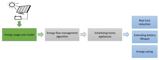
Previous studies focused on optimizing the operation time of home appliances based on minimizing the cost of energy used from the grid. This work focuses on managing home energy consumption using PV and ESS by scheduling the operation time of home appliances considering the installation cost and lifecycle of the PV-ESS. The objective of this work is to achieve realistic cost reduction of using energy, energy savings through efficient energy utilization, and maintaining the integrated system lifespan. The main contributions of this work are the development of battery and PV energy usage cost models; the implementation of a model of selling energy to the grid, and the introduction of the previous steps to an optimization problem. Additionally, creating an efficient energy-flow-management algorithm and a model of a one-minute time slot is considered for the optimization problem, which makes the results more accurate. These contributions consider the installation cost and the lifecycle of the integrated system, which will help with efficient energy utilization and reduce energy losses and wasted energy. Moreover, a real case study was used to obtain realistic results to encourage household energy consumers to manage their energy consumption.

2. Methodology

To accomplish the objectives of this work, the methodology undertaken is as follows:

• Mathematical model formulation of PV, ESSs, and home energy demand.
• Mathematical model formulation of the PV and battery energy-usage cost and selling energy to the grid, considering the PV battery installation cost and lifecycle.
• Algorithm development to obtain an optimal energy flow.
• Objective function development.
• Selection and description of the case study (load profile, solar radiation, PV battery systems size, and grid buying/selling price).
• Optimization algorithms implementation for scheduling home appliances (one-minute operation time interval).
• Selection and analysis of sustainability factors, including modeling and running: expected battery lifespan, carbon emission intensity, and the breakeven point of the system.
• Evaluation of the proposed system’s: simulation by previous scenarios definition and final results obtainment.

3. Development

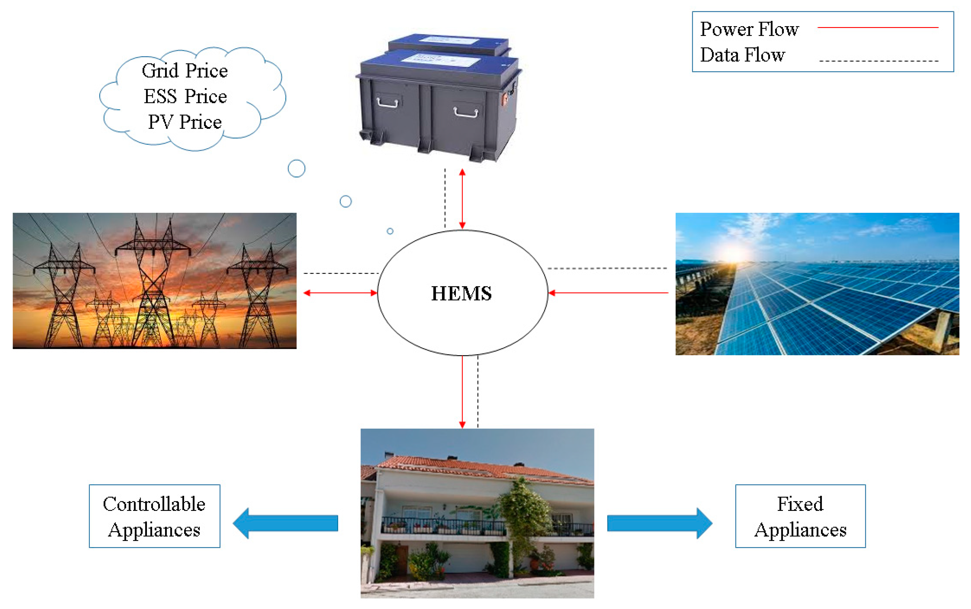
Figure 1 shows the architecture of HEMS, which includes PV, ESS, home appliances, and the main grid. In addition, the data (PV power, PV energy-usage price, battery’s capacity, battery energy-usage price, grid price, and load) flows through the system to manage energy consumption and power flow.

3.1. System Model

3.1.1. PV Generation Model

The PV output power is calculated using Equation (1) [27].

$$P_{PV}\left(t\right)=A\ast \gamma \ast Ir\left(t\right)\ast {\mu }_{conv}$$

(1)

where $P_{PV}\left(t\right)$ is the PV output power (kW) at each time slot t, $A$ is the area of the solar panel (m²) and the efficiency of the PV system is $\gamma$ (%), $Ir$ the solar irradiation (kW/m²), the efficiency of the (DC/AC) inverter ${\mu }_{conv}$, which is assumed to be 97%.

3.1.2. Battery Storage Model

The instantaneous energy in the battery is presented in Equation (2), considering the converter losses during the charging and discharging process [15].

$$E_B\left(t+1\right)=E_B\left(t\right)+P_B^{ch}(t)\ast \eta \ast ∆t-\frac{P_B^{dis}\left(t\right)}{\eta }\ast ∆t$$

(2)

where $E_B\left(t\right)$ represents the amount of current energy in the battery at each time slot t (kWh) and $E_B\left(t+1\right)$ is the amount of energy of the battery in the next time slot t (kWh). $P_B^{ch}\left(t\right)$ denotes the total stored power in the battery (kW) at each time slot t, whereas $P_B^{dis}\left(t\right)$ is the total supplied power from the battery (kW). $\eta$ is the converter efficiency of charging and discharging which is assumed to be 0.95; $∆t$ is the simulation time which is equal to 1 divided by 60.

Equations (3)–(5) are used to calculate the battery energy losses due to converter losses.

$${ch}_{losses}(t)=P_B^{ch}(t)\ast \frac{1-\eta }{\eta }$$

(3)

$${dis}_{losses}\left(t\right)=P_B^{dis}\left(t\right)\ast (1-\eta )$$

(4)

$$B_{losses}\left(t\right)={ch}_{losses}\left(t\right)+{dis}_{losses}\left(t\right)$$

(5)

where ${ch}_{losses}\left(t\right)$ represents the battery charging losses (kW) at each time slot t, ${dis}_{losses}\left(t\right)$ represents the battery discharging losses (kW) at each time slot t, and $B_{losses}\left(t\right)$ refers to the overall battery losses (kW) at each time slot t. Furthermore, ESSs has certain constraints to avoid deep charging and discharging of the battery and some limits for charging/discharging at each time slot t. For this purpose, the constraints in Equations (6)–(8) were set.

$${SOC}_{min}\le SOC\left(t\right)\le {SOC}_{max}$$

(6)

$$0\le P_B^{ch}\left(t\right)\ast ∆t\le {CH}_{rate}$$

(7)

$$0\le P_B^{dis}\left(t\right)\ast ∆t\le {Dis}_{rate}$$

(8)

where $SOC$ represents the ratio of total energy storage to the total energy capacity of the battery (%) at each time slot t, ${CH}_{rate}$ is the maximum charge rate of the battery (kWh) during the time slot t, and ${Dis}_{rate}$ is the maximum discharge rate of the battery (kWh) during the time slot t, which is determined by the battery’s characteristics.

3.1.3. Energy Demand Model

In this work, the household appliances are classified into two categories: fixed and controllable appliances. The set of fixed appliances are presented as X = (b₁, b₂, b₃, …, b_m) over a scheduling duration of t = (1, 2, 3, …, 1440). Equation (9) is used to calculate the total energy consumption of the fixed appliances, and Equation (10) expresses the operating status of the fixed appliances.

$$E_{fixed}(t)=\sum _{X=1}^m{P}_X\ast OP\left(b_X\left(t\right)\right)\ast ∆t$$

(9)

$$OP(b_X\left(t\right))=\left(\begin{array}{c}1,ifthefixedappliance ison\\ 0,ifthefixedappliance isoff\end{array}\right)$$

(10)

where $E_{fixed}\left(t\right)$ represents the total energy consumption of the fixed appliances (kWh) at each time slot t. $P_X$ is the rated power of the fixed appliances (kW), and $OP\left(b_X\left(t\right)\right)$ is a variable that indicates the status of the fixed appliance if it is operating or not at each time slot t.

Controllable appliances are those whose usage can be shifted to off-peak hours. The set of controllable appliances are presented as Y = (c₁, c₂, c₃, …, c_n) over a scheduling duration of t = (1, 2, 3, …, 1440). Equation (11) is used to calculate the total energy consumption of the controllable appliances; Equation (12) expresses the operating status of the controllable appliances.

$$E_{controllable}(t)=\sum _{y=1}^n{P}_Y\ast OP\left(C_y\left(t\right)\right)\ast ∆t$$

(11)

$$OP(c_y\left(t\right))=\left(\begin{array}{c}1,ifthecontrollableappliance ison\\ 0,ifthecontrollableappliance isoff\end{array}\right)$$

(12)

where $E_{controllable}\left(t\right)$ is the total energy consumption of the controllable appliances (kWh) at each time slot t. $P_Y$ is the rated power of the controllable appliances (kW), and $OP\left(C_y\right(t\left)\right)$ is a variable that indicates whether the controllable appliances are operating or not at each time slot t.

The total energy demand $E_{home}^{hourly}\left(t\right)$(kWh) at each time step t is calculated using Equation (13), whereas Equation (14) is used to calculate the total daily demand $E_{home}^{total}$ (kWh).

$$E_{home}^{hourly}\left(t\right)=E_{fixed}(t)+E_{controllable}(t)$$

(13)

$$E_{home}^{total}=\sum _{t=1}^{1440}{E}_{fixed}(t)+\sum _{t=1}^{1440}{E}_{controllable}(t)$$

(14)

3.2. Energy Usage Pricing Model

3.2.1. Battery Energy Usage Price

Batteries play a key role in power system’s stability, balancing supply and demand, and reducing electricity bills. However, batteries have an installation cost. Thus, the battery energy-usage price is modeled and introduced into the optimization problem to use the battery efficiently and enhance its lifespan.

Levelized Cost of Storage

The Levelized Cost of Storage (LCOS) expresses the cost of storing energy in the battery throughout its lifespan. To calculate LCOS, the investment cost of the battery $C_{batt}$ (EUR), the number of cycles $N_{cycle}$, battery Depth of Discharge ($\mathrm{D}\mathrm{O}\mathrm{D}$) (%), and nominal energy of the battery system $E_{batt}$ (kWh) were considered. LCOS is calculated using Equation (15), where the unit of $LCOS$ is EUR /kWh.

$$LCOS=\frac{C_{batt}}{E_{batt}\ast N_{cycle\ast DOD}}$$

(15)

Battery Energy Usage Price

The battery energy-usage price is determined based on the LCOS, and the amount of energy purchased from PV/grid and stored in it. The cost of purchased energy from the PV/grid and stored it in the battery are calculated using Equations (16) and (17), respectively. The total price of purchased and stored energy in the battery ${Ch}_{price}$ (EUR/kWh) in each time slot t is calculated using Equation (18).

$${Pch}_{pv}\left(t\right)=\left(P_{pvtb}\left(t\right)\ast \left({LCOE}_{pv}+LCOS\right)\right)\ast ∆t$$

(16)

$${Pch}_{grid}\left(t\right)=\left(P_{gtb}\left(t\right)\ast \left(G_{Bu{y}_{Price}}\left(t\right)+LCOS\right)\right)\ast ∆t$$

(17)

$${Ch}_{price}\left(t\right)=\frac{{PCh}_{pv}\left(t\right)+{PCh}_{grid}\left(t\right)}{P_{pvtb\left(t\right)}+P_{pgtb\left(t\right)}}\ast ∆t$$

(18)

where ${Pch}_{pv}\left(t\right)$ is the cost of the energy purchased from PV and stored in the battery (EUR) at each time slot t.${LCOE}_{pv}$ denotes the PV energy usage price (EUR/kWh). ${Pch}_{grid}\left(t\right)$ is the cost of energy purchased from the grid and stored in the battery (EUR ) at each time slot t. $P_{pvtb}\left(t\right)$, $P_{gtb}\left(t\right)$ are the amount of PV and grid-stored power in the battery (kW) at each time slot t, respectively. $G_{Bu{y}_{Price}}\left(t\right)$ is the grid price (EUR/kWh) at each time slot t.

The battery energy-usage price varies during the day. The overall price of the battery energy usage is calculated using Equation (19), which is based on the previous price of the battery, the previous amount of energy in the battery, in addition to the new price of purchased energy, and the new amount of purchased energy. Equation (20) expresses the cost of battery energy usage in the home $C_{batt}\left(t\right)$ (EUR) at each time slot t. Where the battery energy losses cost $B_{LC}\left(t\right)$ due to the energy losses (EUR) during the process of charging the battery from the grid/PV, and discharging the battery to the home/grid, taking into account the energy prices and amount of charged/discharged energy at each time slot t is calculated using Equation (21).

$$B_{price}\left(t+1\right)=\frac{{(B}_{price}\left(t\right)\ast P_b\left(t\right)){+(Ch}_{price}\left(t\right)\ast (P_{pvtb}\left(t\right)+P_{gtb}\left(t\right)\left)\right)}{P_b\left(t\right)+P_{pvtb}\left(t\right)+P_{gtb}\left(t\right)}$$

(19)

$$C_{batt}\left(t\right)=B_{price}\left(t\right)\ast P_{bth}\left(t\right)\ast ∆t$$

(20)

$$B_{LC}\left(t\right)=\left\{\begin{array}{c}\left[P_{gtb}\left(t\right)\ast \frac{1-\eta }{\eta }\ast G_{Bu{y}_{Price}}\left(t\right)\right]+\left[P_{PVtb}\left(t\right)\ast \frac{1-\eta }{\eta }\ast {LCOE}_{pv}\right]\\ +\left[P_{bth}\left(t\right)\ast \left(1-\eta \right)\ast B_{price}\left(t\right)\right]+\left[P_{btg}\left(t\right)\ast \left(1-\eta \right)\ast B_{price}\left(t\right)\right]\end{array}\right\}\ast ∆t$$

(21)

where $B_{price}\left(t+1\right)$ expresses the price of battery energies (EUR/kWh) for the next time slot (t + 1) after adding the new charged energy price ${Ch}_{price}\left(t\right)$, where $B_{price}\left(t\right)$ is the price of the battery energy usage (EUR /kWh) in the time slot t, and $P_b\left(t\right)$ express the battery net power at the time slot t (kW). $P_{bth}\left(t\right)$, $P_{btg}\left(t\right)$ express the amount of power sent from the battery to the home and grid (kW) at each time slot t, respectively.

3.2.2. PV Energy Usage Price

PV supplies energy to the load and battery and sells to the grid. To ensure that PV is used efficiently throughout its life cycle, the Levelized Cost of Energy (LCOE) of PV is expressed as the price of PV energy usage price; this price takes the installation cost and overall Operation and Maintenance (O&M) expenses into account. The cost of PV energy consumed in the home $C_{PV}\left(t\right)$ (EUR) at each time slot t is calculated using Equation (22), where $P_{Pvth}\left(t\right)$ is the amount of PV power usage in the home (kW) at each time slot t.

$$C_{PV}\left(t\right)={LCOE}_{pv}\ast P_{Pvth}\left(t\right)\ast ∆t$$

(22)

3.2.3. Selling Energy to the Grid

In the process of selling energy to the grid, the profit is expressed based on the PV, battery, and grid energy usage prices to obtain efficient energy management that considers the installation cost and lifespan of systems. Equation (23) calculated the profit of selling energy from PV to the grid, taking into account the grid prices at each time slot t and LCOE. The higher the grid-selling price compared to the LCOE, the greater the profit. The same applies for selling energy from the battery to the grid; Equation (24) calculated the profit. The higher the grid-selling price compared to the battery price, the greater the profit. These equations express the real profit of selling energy; thus, they are introduced into the optimization problem. The overall profit of selling energy to the grid ${Profit}_{sell}\left(t\right)$(EUR) at each time slot t is calculated using Equation (25).

$${Profit}_{pvtg}\left(t\right)={\left(\right(P}_{pvtg}\left(t\right)\ast ({Grid}_{sell}\left(t\right)-{LCOE}_{pv}))\ast ∆t$$

(23)

$${Profit}_{btg}\left(t\right)=(P_{btg}\left(t\right)\ast ({{Grid}_{sell}\left(t\right)-(B}_{price}\left(t\right)\left)\right)\ast ∆t$$

(24)

$${Profit}_{sell}\left(t\right)={Profit}_{pvtg}\left(t\right)+{Profit}_{btg}\left(t\right)$$

(25)

where ${Profit}_{pvtg}\left(t\right),{Profit}_{btg}\left(t\right)$ represents the economic benefit of selling energy from PV and battery to the grid (EUR) at each time slot t, respectively. $P_{pvtg}$ represents the amount of PV power sent to the grid (kW) at each time slot t, and ${Grid}_{sell}$ is the energy selling price to the grid (EUR /kWh) at each time slot t.

3.3. Energy Flow Management Algorithm Development

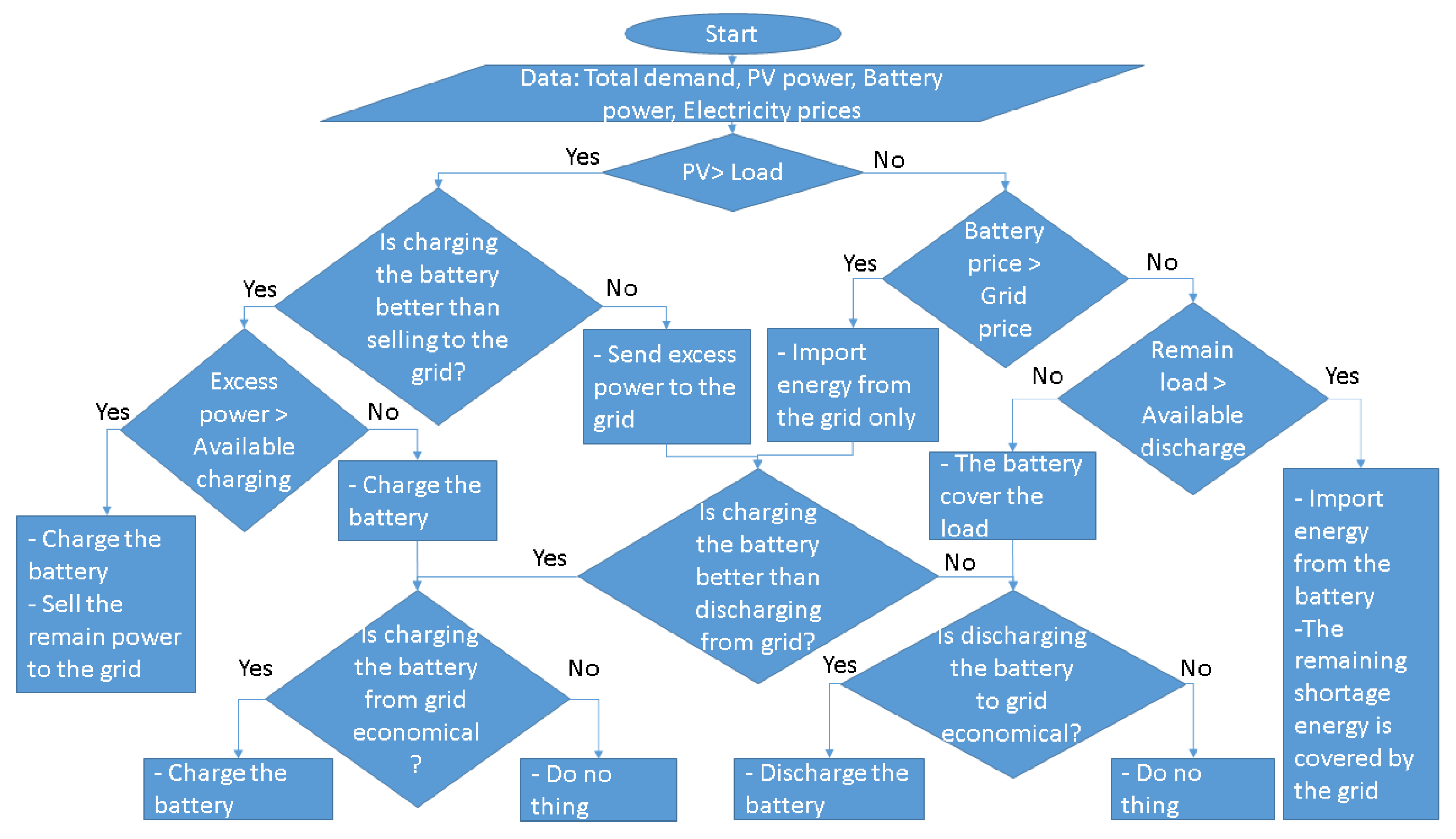
Figure 2 illustrates the Proposed Energy Flow Management Algorithm (PEFMA). It considers the life cycle of the battery and PV by using them efficiently. At first, PV provides power to the appliances. During the periods of excess PV generation, PEFMA compares the economic benefit of storing the excess energy in the battery to use it during the grid high price periods (grid high price − (LCOS + LCOE)) versus selling the excess energy to the grid (LCOE − grid selling price). If the economic benefit of storing the excess energy in the battery is higher than selling it to the grid, PEFMA will store the excess energy in the battery. Otherwise, PEFMA will sell the excess energy to the grid.

If the PV generation is insufficient to meet the load, PEFMA compares the battery energy-usage price against the grid price to determine the best alternative. If the battery price is lower than the grid price, PEFMA will give priority to the battery to cover the load, then to the grid. Otherwise, PEFMA will cover the load from the grid only.

Battery charging/discharging from/to the grid considers the battery life cycle as well as the economic gain. For each possible period of charging the battery from the grid, PEFMA checks if the cost of storing energy (LCOS + grid price) is lower than the grid high price; if it is, PEFMA will charge the battery from the grid. Otherwise, the battery will not be charged because it will not be beneficial for future use. For each possible period of discharging the battery to the grid, PEFMA checks if the economic benefit of selling battery energy to the grid (grid selling price–battery price) is higher than discharging it to cover the load in the grid high price period (grid high price–battery price); if it is, PEFMA will sell the battery energy to the grid. Otherwise, the battery will not be discharged.

3.4. Objective Function

The main aim of this work is to schedule the home appliances and manage the energy flow considering the installation cost and life cycle of PV and battery. The energy usage cost of using PV and battery is modeled and considered in the objective function. Moreover, the profit from selling energy to the grid is considered in the objective function. Equation (26) represents the objective function of the optimization strategy; it aims to minimize the real energy cost by scheduling the home appliances and using the battery, PV energy, and grid utilization optimally. $C_{Grid}\left(t\right)$ expresses the cost of power imported from the (EUR) at each time slot t.

$$Minimize\left(RealCost\right)=Min\sum _1^{1440}{C_{Grid}\left(t\right)+C}_{PV}\left(t\right)+C_{batt}\left(t\right)-{Profit}_{sell}\left(t\right)$$

(26)

The objective function is subjected to the constraints of user preferences based on the minimum/maximum starting time of each controllable appliance, as shown in

Table 1. Home electrical appliances description.

Appliance	Rated Power (kW)	Category	Priority	Start Time (St)	End Time (Et)	Min. Start Time	Max. Start Time
Xbox	0.072	Controllable	Low	22	00	19	23
TV (Living room)	0.069	Controllable	Low	14	18	15	18:00
Electric fryer	2.2	Controllable	High	14 & 15	14:15 & 15:15	11:30 & 14:30	14 & 16
Oven	2.5	Controllable	High	12 & 17	12:30 & 17:30	10:30 & 16:00	12 & 18
Dishwasher	0.9	Controllable	Low	18	20	18	22
Washing Machine	0.579	Controllable	Low	09	11	08	22
Iron	2.6	Controllable	Low	19	19:30	08	22
Vacuum cleaner	0.8	Controllable	Low	13	13:30	08	22
Ceramic cooktop	5.7	Controllable	-	13	13:25	-	-
TV (Bedroom)	0.12	Fixed	-	20	22	-	-
TV (Kitchen)	0.12	Fixed	-	12	14	-	-
Coffee machine	1.25	Fixed	-	08 & 19	8:15 & 19:15	-	-
Microwave	1	Fixed	-	08 & 20	8:15 & 20:15	-	-
Fridge	0.1	Fixed	-	00	23	-	-
Laptop Lenovo	0.035	Fixed	-	14	18	-	-
Laptop HP	0.045	Fixed	-	00	00	-	-
Mobile chargers	0.054	Fixed	-	01 & 15	03 & 17	-	-
Light bulbs	0.124	Fixed	-	00 & 08	01 & 00	-	-

. The priority of each controllable appliance to be shifted is classified into low and high. The low-priority appliances have the possibility to schedule the starting operation time within a period that is longer than the high-priority appliances’ period. The user sets the controllable appliances, their minimum/maximum starting time, and the priority of each appliance.

3.5. Case Study

The load data of a home in Vigo (Spain) are used as a case study, where the user determined the category and operating time constraints of the home appliances as shown in Table 1. The PV system of 1.035 kWp size is used, where the solar radiation data were collected from the PVGIS 5.2 database of Vigo [28]. Figure 3 shows the power demand, PV power generation throughout the day, and the grid prices [29,30]. The average data for two months in the summer (June and July) of solar radiation and grid prices are taken.

The battery system with a capacity of 2.4 kWh is employed, starting with a 0% initial state of charge. The LCOS is calculated using Equation (11), where the battery cycles are 6000 with 80% DOD [31]. It is found that LCOS is equal to 0.072 EUR/kWh. According to the International Renewable Energy Agency (IREA), the LCOE of PV is 0.092 EUR/kWh for the Spanish residential sector in 2020 [32].

3.6. Optimization Algorithms

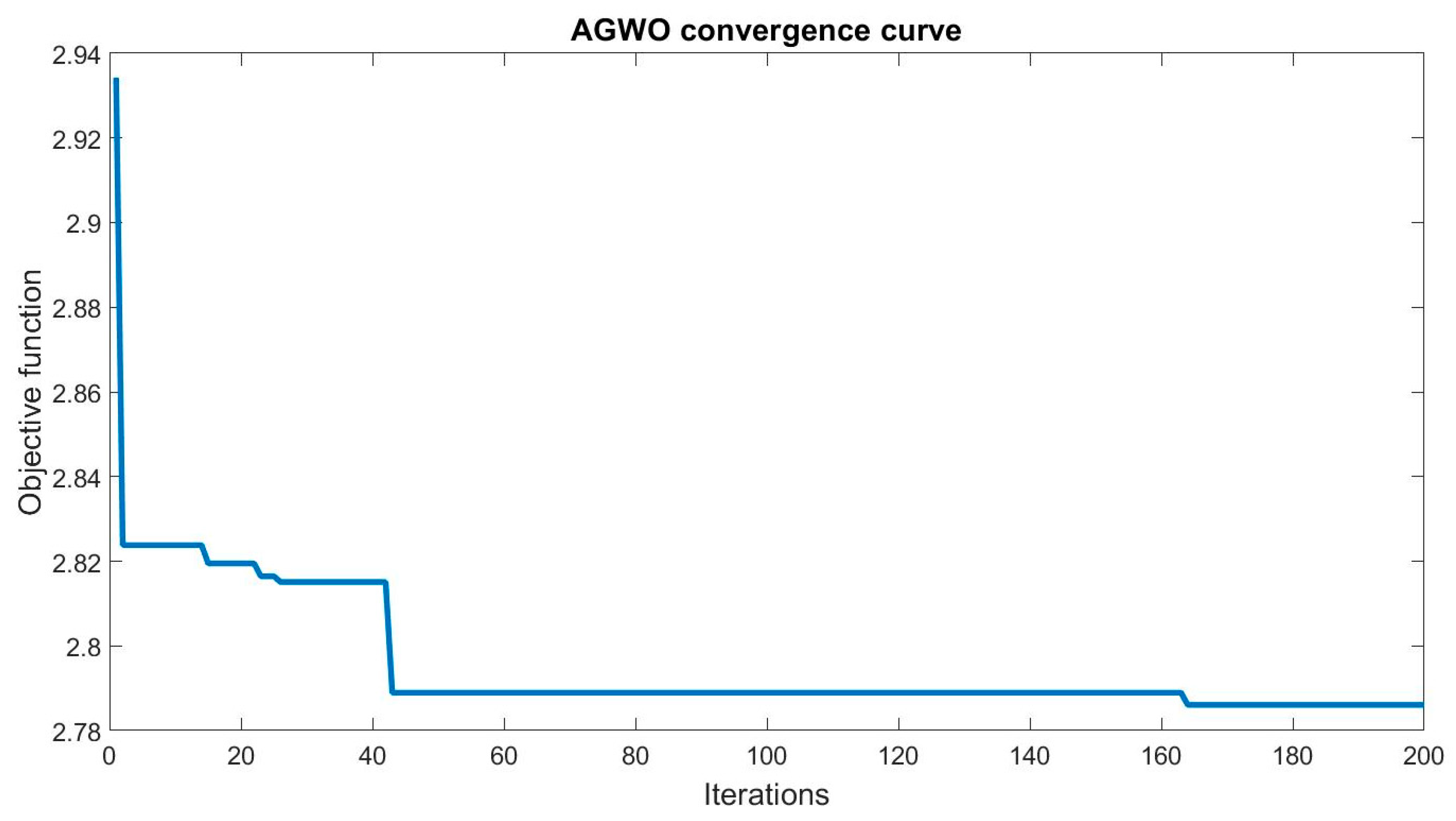
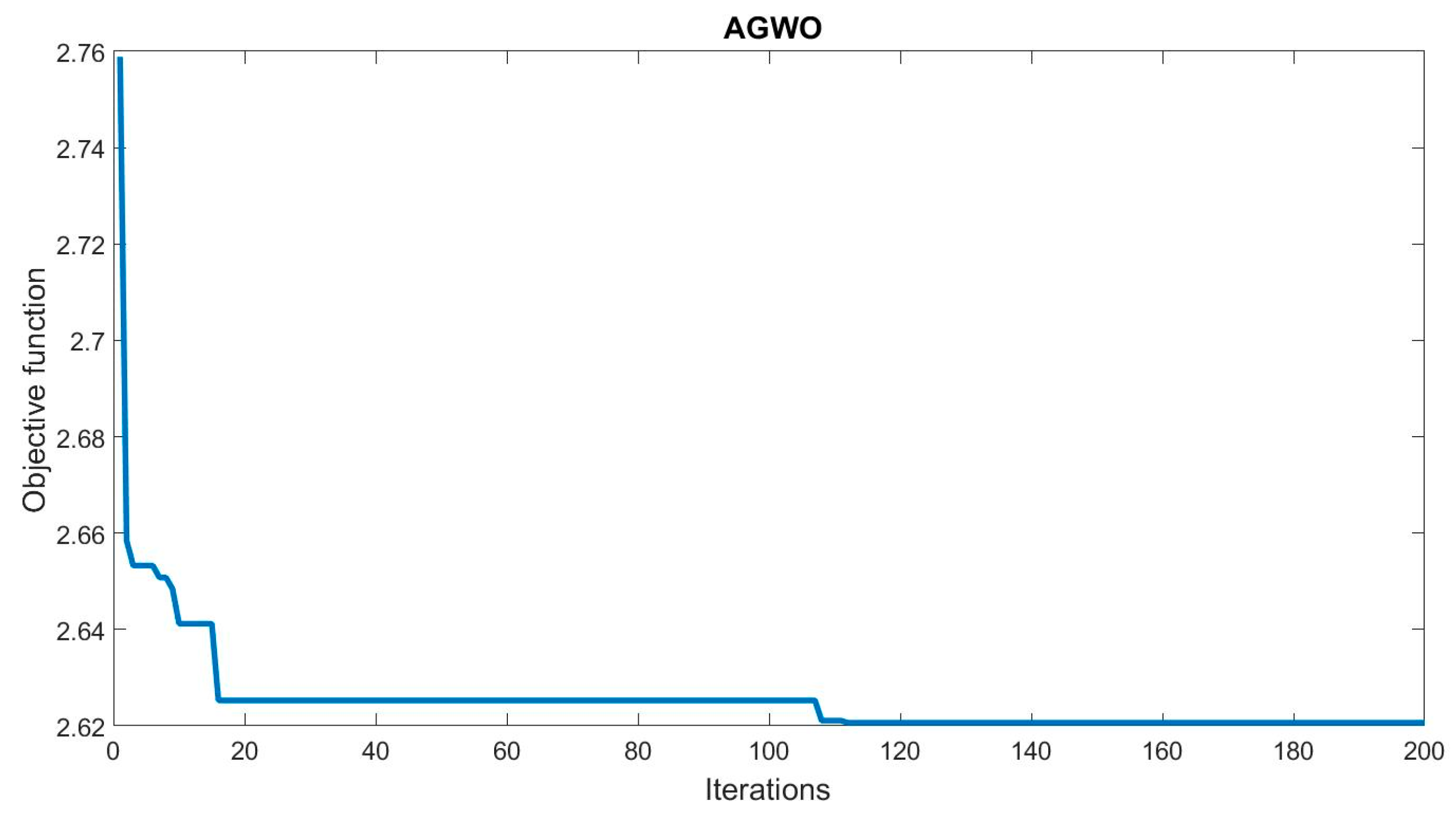
3.6.1. Augmented Gray Wolf Optimization Algorithm

The grey wolf optimizer (GWO) is a meta-heuristic algorithm inspired by the community formed by wolf packs, which are based on hunting behavior and their social leadership [33]. There are four levels of wolf packs, and the leader of the whole pack, the alpha wolf (α), supervises several tasks such as hunting, searching for a sleeping place, and determining the time to wake. The second level is beta wolves (β), which possess the traits of a leader in the case of the alpha wolf becoming old or passing away, as well as acting as an advisor to the alpha and giving commands to the lower levels of the wolves’ pack. The third level is delta wolves (δ) which ensure the safety and well-being of the pack, supervised by alpha wolves and beta wolves, and participate in hunting and decision-making tasks. Finally, the lowest level of the grey wolf pack is omega wolves (ω), which act as scapegoats, i.e., all the other wolves in the pack rule them. However, the GWO was developed into an Augmented GWO (AGWO) [34]. Unlike GWO exploration and exploitation α based, where this parameter changes linearly from 0–2, AGWO α based changes nonlinearly and randomly within the range 1–2. Furthermore, in AGWO, hunting and decision-making are solely based on the updating of α and β, unlike GWO, which is dependent on α, β and δ. These improvements allow AGWO to possess greater exploration capabilities in comparison with GWO.

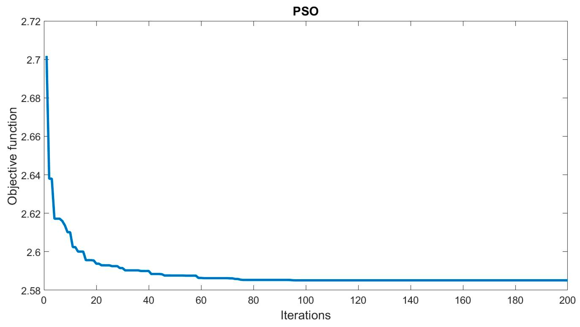
3.6.2. Particle Swarm Optimization Algorithm

PSO is a metaheuristic optimization algorithm inspired by the social behavior of bird flocking or fish schooling developed in 1995 by Eberhart and Kennedy [35]. PSO involves a population of particles moving through a search space to find the optimal solution to an optimization problem. Each particle represents a potential solution and adjusts its position and velocity based on its own experience and the collective knowledge of the swarm. By continuously updating their positions and velocities, particles explore and exploit the search space, converging towards the global optimum. Its effectiveness lies in the cooperation and information sharing among particles, allowing them to collectively search the solution space and converge towards the global optimum. Besides, PSO is known for its simplicity and effectiveness in solving various optimization problems.

3.7. Analysis of Sustainability Factors

3.7.1. Battery Lifespan

One of the aims of this study is to sustain the battery’s lifespan, which is influenced by a number of charge–discharge cycles [36]. Each battery has a number of cycles throughout its lifespan; a single cycle means that the battery is being charged to full capacity and then drained to empty either in a single sitting or at irregular intervals. Therefore, the number of charging/discharging cycles throughout the day $B_{daycycles}$ is calculated using Equation (27), and the expected lifespan of the battery $B_{life}$ (in years) which is based on the number of battery cycles specified by the manufacturer over its lifespan $N_{cycle}$, calculated using Equation (28) where $d_y$ represents the number of days in one year.

$$B_{daycycles}=\frac{\sum _1^{1440}{P}_B^{ch}\left(t\right)\ast ∆t+\sum _1^{1440}{P}_B^{dis}\left(t\right)\ast ∆t}{E_{batt}}$$

(27)

$$B_{life}=\frac{N_{cycle}}{B_{daycycles}\ast d_y}$$

(28)

3.7.2. Carbon Emission Intensity

The fossil fuel power plants have negative environmental and human health effects, and the residential sector can help reduce CO₂ emissions by adopting local RESs and scheduling home energy consumption. The amount of ${\mathrm{C}\mathrm{O}}_2$ emissions is calculated using Equation (29). $P_{gth}\left(t\right)$ is the amount of grid power sent to the home at each time step t (kW), while $I_{{CO}_2}$ expresses the carbon emission intensity of electricity generation. In the case of Spain, $I_{{CO}_2}$ is equal to 0.177 (kgCO₂/kWh) in 2020 [37].

$${\mathrm{C}\mathrm{O}}_2=I_{{CO}_2}\mathrm{*}\sum _{t=1}^{1440}(P_{gth}\left(t\right)+P_{gtb}\left(t\right))$$

(29)

3.7.3. Breakeven Point of the Integrated System

The breakeven point of the PV battery system refers to the point at which the installation cost equals the financial benefits it gained over its lifetime. In other words, it is the point at which the savings from electricity generation offset the system’s initial investment and ongoing expenses. The following model calculates the expected breakeven point of the proposed system. Equation (30) shows the daily saved cost $d_{saving}$ calculation during the battery lifespan and after the battery lifespan, only PV supports the load. Equation (31) is used to calculate the overall saved cost ${PVB}_{saving}$ during the battery lifespan integrating with PV (EUR). The PV daily cost saving ${PV}_{saving}$ after the battery stops working (EUR/day) is calculated using Equation (32). Equation (33) is used to calculate the expected breakeven point of the PV battery system $Y_{BP}$ (in years).

$$d_{saving}=\left(\begin{array}{c}{PVB}_{saving}, duringthebatterylifespan\\ {PV}_{saving}, afterthebatterystopsworking\end{array}\right)$$

(30)

$${PVB}_{saving}=\sum _1^{B_{life}}(B_{cost}-{Sch}_{cost})$$

(31)

$${PV}_{saving}=\sum _{t=1}^{1440}\left(P_{pvth}\left(t\right)\ast G_{{Buy}_{price}}\left(t\right)\right)+\left(P_{pvtg}\left(t\right)\ast {Grid}_{sell}\left(t\right)\right)\ast ∆t$$

(32)

$$Y_{BP}=\left(B_{life}+\frac{{Inv}_{sys}-{PVB}_{saving}}{{PV}_{saving}}\right)/365$$

(33)

where $B_{cost}$ denotes the electricity cost without using the PV battery system, ${Sch}_{cost}$ express the scheduling strategy electricity cost (EUR ). ${Inv}_{sys}$ express the investment cost of the installed PV battery system (EUR), and $B_{life}$ unit is days.

4. Results: Evaluation of the Performance of the Proposed System

AGWO and PSO algorithms are used to solve the optimization problem with 100 populations, and 200 iterations. For simulations, we used MathWorks MATLAB R2021a for academic use, installed on Intel(R) Core(TM) i7-3520M CPU @ 2.90GHz and 8 GB RAM with Windows 10 Pro. Each simulation run needed seven hours to finish the 200 iterations and obtain the best solutions. Four scenarios were simulated to evaluate the effectiveness of the proposed optimization strategy and the PEFMA.

4.1. The Base Scenario (The First Scenario)

In this scenario, the home energy demand is covered by the main grid. The total daily demand is 18.464 kWh, with 3.268 kgCO₂, and the total daily electricity cost is EUR 3.7584. The results of the base scenario are used to compare them to the proposed system and other scenarios.

4.2. The Proposed Energy Flow Management Algorithm (The Second Scenario)

The PEFMA manages the distribution of energy in an effective manner, considering the grid prices, LCOE and LCOS. As shown in Figure 4, during the periods 08:01–10:00 and 17:01–17:30, importing energy from the grid is preferable to importing energy from the battery. However, during the periods 10:01–11:00 and 18:01–19:00, using battery energy is preferable to importing energy from the grid. Figure 5 shows the energy balance of the system: the battery sold no energy to the grid, where the cost of battery’s energy usage is higher than the grid-selling price. The same behavior is observed for PV owing to the low selling price, often less than LCOE: it is preferable to supply the PV power to the home or store it in a battery rather than sell it to the grid. The results show that the real cost is EUR 3.163. The total charged and discharged battery energy is 9.047 kWh, the battery losses amount to 0.46771 kWh, and the battery losses cost is EUR 0.071, where the estimated battery lifespan is 4.36 years. The amount of CO₂ emissions is 2.79 kgCO₂.

4.3. The Proposed Optimization Strategy (the Third Scenario)

In this scenario, the objective function includes the cost of battery energy usage, the cost/profit of imported/sold energy from/to the grid, and the PV energy usage cost. The simulation results of AGWO show that the real cost is EUR 2.786. The total charged and discharged battery energy is 8.447 kWh, the battery losses amount to 0.436 kWh and the battery losses cost is EUR 0.06424, where the estimated battery lifespan is 4.67 years. In addition, the amount of CO₂ emissions is 2.773 kgCO₂. In the case of PSO, the real cost is EUR 2.782. The total charged and discharged battery energy is 7.6687 kWh, the battery losses amount to 0.397 kWh and the battery losses cost is EUR 0.059, where the estimated battery lifespan is 5.14 years. In addition, the amount of CO₂ emissions is 2.755 kgCO₂. Figure 6 and Figure 7 show the convergence of the AGWO and PSO algorithms. Figure 8 shows the energy balance of the system.

4.4. A Previous Study Scheduling Strategy (The Fourth Scenario)

To evaluate the proposed system, a previous study on appliances scheduling strategies is modeled and compared to it. Bouakkaz et al. (2021) modeled a battery energy usage price based on the SOC of the battery and included it in the optimization problem for scheduling the household appliances, where the battery energy price increases when the SOC is low and decreases when the SOC is high [26]. They attempted to use the battery more efficiently with fewer energy losses. We applied Bouakkaz et al. (2021) scheduling strategy to the same data in this scenario, using the same objective function based on their energy usage-pricing model [26]. After determining the optimal appliances’ operation time, we calculated the real electricity cost. The results of AGWO show that the real cost is EUR 3.029. The total charged and discharged battery energy is 14.2159 kWh, the battery losses amount to 0.7319 kWh, and the battery losses cost is EUR 0.092, with an estimated battery lifespan of 2.775 years. In addition, the CO₂ emissions are 2.553 kgCO₂. In the case of PSO, the real cost is EUR 3.025, the total charged and discharged battery energy is 14.165 kWh, the battery losses amount to 0.729 kWh, and the battery losses cost is EUR 0.0945, with an estimated battery lifespan of 2.785 years. In addition, the CO₂ emissions are 2.576 kgCO₂.

Figure 9 and Figure 10 show the convergence of the AGWO and PSO algorithms. It is observed that the minimum electricity cost is lower than the real electricity cost; this is because the Bouakkaz et al. [26] model did not consider the battery’s LCOS and PV’s LCOE. This led to inefficient utilization of energy. Figure 11 shows the energy balance of the system.

5. Discussion

Four scenarios were carried out to show the effectiveness of the proposed system in reducing cost by scheduling the appliances with efficient usage of the battery and PV, maintaining the system’s lifespan. This section discusses the obtained behavior in terms of the real electricity cost, battery lifespan, energy losses, energy usage cost pricing, and breakeven point. In addition, we compared our proposed system to a previous work of energy usage cost using AGWO and PSO.

5.1. Cost

Figure 12 describes the comparison simulation results of the real electricity cost and cost reduction compared to the base scenario using AGWO and PSO. In both cases of AGWO and PSO, the proposed system (third scenario) has achieved the best cost reduction: 28.87% using AGWO and 25.98% for PSO. The fourth scenario reduces the cost by 19.4% for AGWO, and 19.51% for PSO.

5.2. Battery Lifespan and Energy Losses

Figure 13 illustrates the comparison of battery lifespan and energy loss results of the third and fourth scenarios using AGWO and PSO. The results show that the proposed system accomplished the most extended battery lifespan of 4.67 years and 5.14 years using the AGWO, and PSO, respectively, while the AGWO and PSO results of the fourth scenario show that, the battery lifespan is 2.775 years, 2.785 years, respectively. Compared to Bouakkaz et al. [26] strategy in the fourth scenario [26], the proposed system extends the battery lifespan by 68.282% and 84.56% in the case of AGWO and PSO, respectively. Moreover, the proposed system achieves the fewest energy losses compared to the fourth scenario. In the case of AGWO, the energy losses of the third and fourth scenarios are 0.436 kWh and 0.7319 kWh, respectively. The proposed system reduces energy losses by 40.429%. Similarly, the energy losses using PSO in the third and fourth scenarios are 0.397 kWh and 0.729 kWh, respectively. The PSO reduces energy losses by 45.540%. This indicates the effectiveness of our proposed system in saving energy and maintaining the battery lifespan.

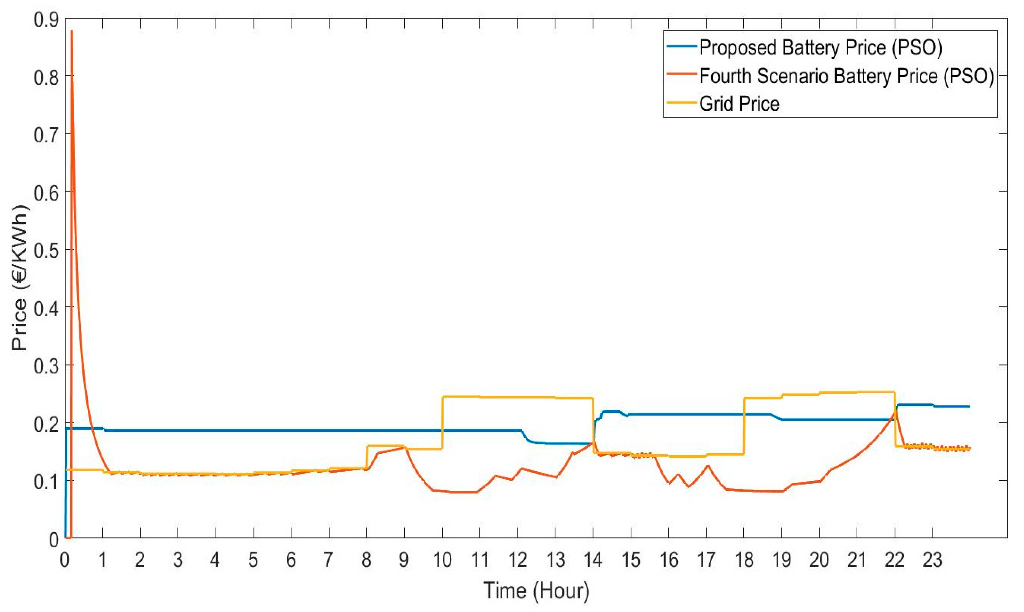
5.3. Energy Usage Prices

The battery energy price of Bouakkaz et al. (2021) in the fourth scenario is far from the real price [26]. On several occasions, the battery price was lower than the grid price, which led to long use of the battery energy and scheduling the appliances more in the battery’s low-price periods. In the case of the battery’s high-price periods with a low amount of energy, the battery does not contribute to covering the load demand even if the grid price is high in reality. For example, at 8 a.m. the grid price is EUR 0.121/kWh, and the proposed battery energy price is EUR 0.192/kWh, whereas the battery energy price of the fourth scenario is EUR 0.118/kWh at SOC 60.8%. This leads to inefficient use of the battery, where the actual price of the battery is based on LCOS and the cost of the energy stored in it, which is equal to EUR 0.192/kWh. In addition, the grid energy price is actually lower than the real battery price. Thus, the proposed system operates the battery in an efficient manner in terms of the battery energy losses and maintaining its lifespan and cost reduction compared to the fourth scenario. The findings demonstrate that the proposed system successfully addresses these issues and presents an optimization strategy that yields superior results, as detailed in the results and discussion sections. Figure 14 shows the energy usage price of the third and fourth scenarios.

5.4. Breakeven Point

The cost of installing a PV battery system depends on the system size and components type of the system. In this study, the investment cost of the PV battery system is assumed to be EUR 2000 according to the market prices [38]. Using the mathematical model in Section 3.7.3, we calculated the expected breakeven point of the PV battery system. As shown in Figure 15, the results demonstrate that the proposed system reached the breakeven point in a shorter time compared to the fourth scenario. In the case of AGWO, the breakeven points of the proposed system and fourth scenario are 4.26 years and 4.32 years, respectively. Similarly, the results of PSO illustrated that the proposed system reached the breakeven point in 4.09 years, while the fourth scenario needed 4.25 years.

The results of the AGWO and PSO show that the proposed system reached the breakeven point in a short time compared to the fourth scenario. Moreover, the results show that the proposed system reached the breakeven point before the battery stopped working; the AGWO extended the battery lifespan of 4.67 years with a 4.26-year breakeven point, and the PSO extended the battery lifespan of 5.14 years with a 4.09-year breakeven point. This indicates that the proposed system is economical and sustains the battery lifespan, where the battery remains functional even after the system reaches the breakeven point, in contrast with the fourth scenario, where the battery ceases to operate before the breakeven point is reached by around 1.5 years.

6. Conclusions and Future Work

This paper proposes an efficient optimization method of scheduling appliances in conjunction with an efficient energy flow management system that considers PV and battery life cycles, as well as installation costs. Battery and PV energy usage pricing models are proposed and considered in the optimization strategy and energy flow management system. For optimization, we used AGWO and PSO algorithms in MATLAB. Real data were used for a house in Vigo, Spain, to provide realistic results that encourage Spanish customers to manage their energy consumption after the new electricity tariff in Spain. To show the effectiveness of the proposed system, a comparison is applied with a previous model of pricing energy usage. The proposed system accomplishes a better reduction in cost and energy losses, a longer extension to the lifespan of the battery, and reaches the breakeven point in a short time. In addition, it encourages energy consumers to contribute to grid stability and energy security by highlighting the economic and environmental benefits of scheduling appliances in conjunction with using PV and batteries during their lifespan compared to their installation costs. In the future, the authors propose the possibility of studying the energy consumption reduction cost with the integration of electric vehicles. Furthermore, it is recommended to expand the scope of the study by incorporating multiple homes to study the mechanism of energy exchange between them, considering the preferences of each user. Additionally, it is suggested that thermostatically controlled loads be integrated into the energy demand model.