Combining Markowitz Portfolio Model and Simplex Algorithm to Achieve Sustainable Land Management Objectives: Case Study of Rivadavia Banda Norte, Salta (Argentina)

Abstract

Land use planning involves making an appropriate decision and selecting a use over other alternatives. A step-by-step methodology was developed to evaluate the optimal combination of regional land use technologies and the spatial allocation. For a realistic approach, a case study (specifically Rivadavia department, Salta, Argentina) is considered, which has deforestation problems and the advance of intensive and extractive agriculture. Five management techniques are considered for the area: precision agriculture (T1), advance livestock farming (T2), payment for ecosystem service (T3), traditional agriculture–livestock farming—Criollo (T4), and traditional forest management—Wichi (T5). A land evaluation on a GIS model is carried out to obtain the land suitability for each technique. Analyzing local experts’ opinions using the Markowitz portfolio methodology allows us to obtain an optimal combination of techniques. Finally, a Simplex method analysis linked with the GIS is performed to allocate the five techniques over the territory maximizing land suitability and in compliance with percent surface assignments. The result assigns each GIS polygon to a specific technique, reaching optimal land suitability in 92% of the territory. Natural capital and social attributes had a significant and complex impact on technology choice, but objective and optimized approaches in their allocation were possible and provides valuable information to guide public policies.

1. Introduction

The Argentinean Chaco has suffered an intense deforestation process. The enlargement of agricultural boundaries and the extraction of goods by big wood enterprises have accelerated this process. These problems threaten the sustainability of the region [1]. Deforestation affects Indigenous groups (such as the Wichis), who depend on the forest. Many projects by nongovernmental organizations and state agencies have sought for the Wichis to implement sustainable agriculture on their lands. However, these have not been very successful because of the worldview of the Wichis, which is more related to hunting and gathering.

Intensive and extensive agricultural activities have put so much pressure on natural resources that they have caused real environmental disasters and heavy polluting emissions. According to [2], agricultural land use accounts for 6% of the United States’ greenhouse gas (GHG) emissions. This percentage is expected to be higher in Latin America, where agriculture is one of the main economic activities, especially in Argentina. Land management activities have great potential for reducing GHG emissions and capturing additional carbon in the soil and biomass.

Land use change (LUC) has a negative impact on ecosystem services and human well-being. The conversion of a native forest to cultivated land could result in changes in soil properties, affecting the hydrological balance [3]. Additionally, it could be one of the most critical sources of carbon released into the atmosphere [4,5]. LUC is one of the main stressors of ecology and biodiversity conservation [6]. However, the effect is the opposite if the change goes from agricultural use to forestry or agroforestry.

Land use planning involves making an appropriate decision and selecting a use over other alternatives. Based on a deep understanding of the consequences, both positive and negative, that derive from this decision, land planning seeks to maximize the benefits and minimize the risks (social, ecological, and economic) and always following the current legal regulations [7,8].

The success of agricultural land planning consists of assigning fair use to each piece of land to obtain the maximum profit and the minimum ecological impact [9]. In this way, it is necessary for a land evaluation that assesses soil, topographic, and climatic characteristics for a defined use, directing agriculture and livestock to suitable lands and keeping unperturbed zones with ecological and hydric conservation interests [10].

Integrating agricultural production and ecosystem conservation is an exciting alternative in sustainable development, both from an ecological and economic perspective, over the long term [11]. This is imperative in a region like Salta with a considerable population of indigenous people whose livelihood depends on forest conservation [12]. This model of a sustainable economy is replacing traditional economic development.

After a land evaluation has been conducted, it may be found that a portion of land is suitable for several uses, and farmers or decision-makers are faced with a dilemma of which of them is the most appropriate use or if a combination of uses is possible [13]. It is widely known that investing in only one activity lets farmers progress rapidly. Nevertheless, it is also efficient to diversify their effort in many simultaneous projects to reduce the risk of losses [14]. Diversification is also considered a climate change adaptation measure that increases farmers’ resilience to extreme climatic events [15].

Ref. [16] analyzed an optimization model for agroecosystem planning and the relationship between socioeconomic viability and biodiversity. The base study considered environmental conditions, such as luminosity, water, and nutrients, and additional financial information on the vegetal, natural, or commercial yield. They found the right crop and plant combination for an agricultural area through the Markowitz model, optimizing their yield, risk, and sustainability objectives. In these cases, optimized agricultural planning is a fundamental activity that allows farmers to obtain an optimal distribution with greater profitability and a low ecological cost [17].

The Markowitz portfolio model [18], derived from the financial field, allows for analyzing return and risk combinations to generate a set of efficient investment portfolios. It has been used to model diversified land use, reducing the risk associated with crop production [19,20] and agroecosystem planning [16]. In addition, there can be significant potential gains from combining varieties or species characterized by an inverse yield response to environmental fluctuations, such as drought, pests, or disease [21,22].

An efficient tool for optimized spatial distribution problems is linear programming, and [23,24,25] indicated that geographical information systems (GIS) is lately a primary tool for a wide variety of earth science and land use applications. Ref. [26] mentioned the potential of integrating optimization methods (specifically, linear programming) with GIS in land use planning. The advantages of combining these technologies are the reduction in time and more accurate results than if only spatial and cartographic methods were used. Among the linear programming methods, the Simplex method is one of the most widely used in many fields and is easy to implement.

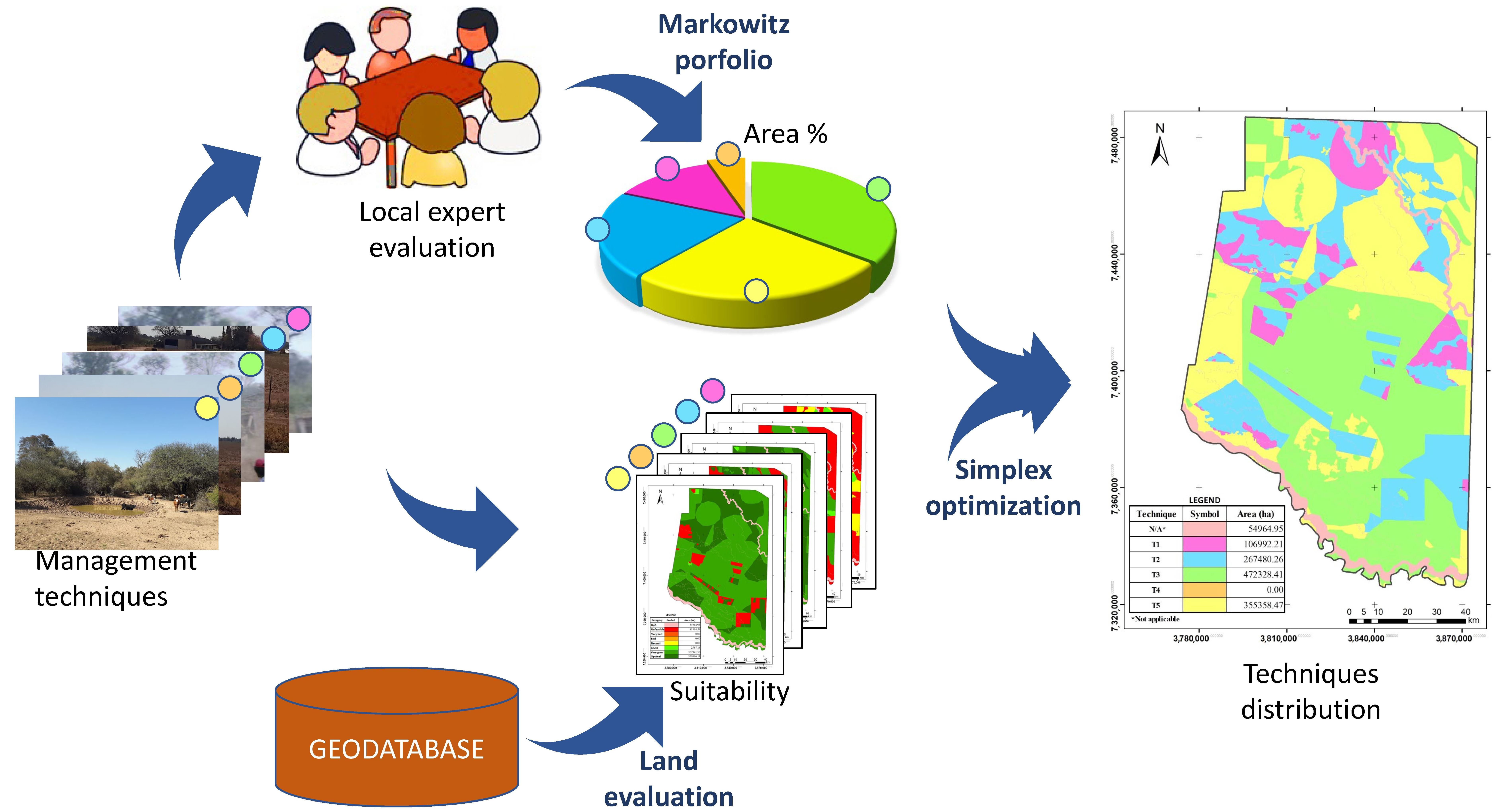
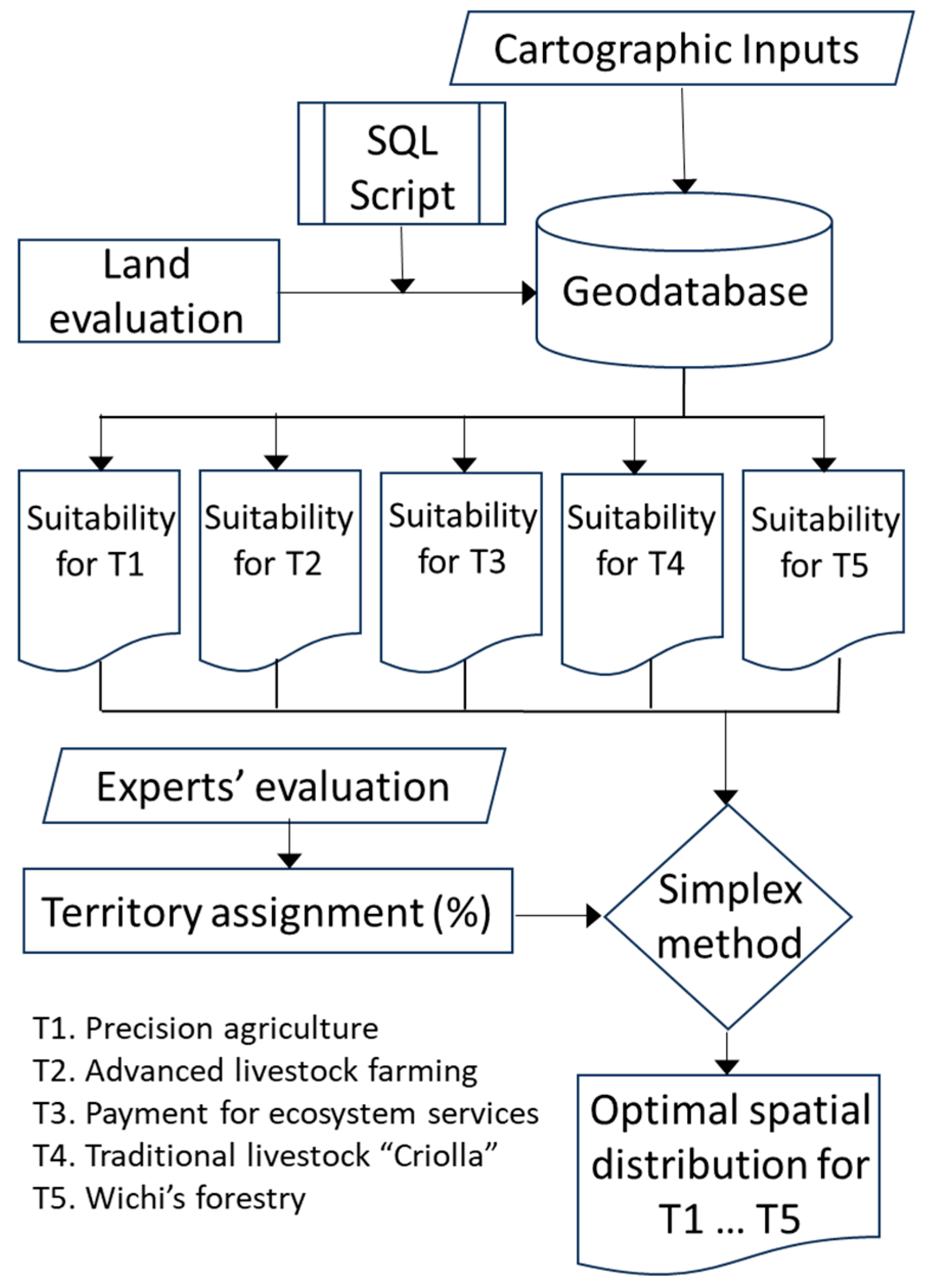
For a realistic approach to a case study (specifically Rivadavia department, Salta, Argentina), we based our work on ten spatially distributed variables describing soil, land coverage and use, and socioeconomic characteristics. Also, an expert panel was selected in the previous first stage of this study to qualify five different techniques for land management, and the agreement among its answers was analyzed [27]. These techniques were precision agriculture (T1), advance livestock farming (T2), payment for ecosystem service (T3), traditional agriculture–livestock farming—Criollo (T4), and traditional forest management—Wichi (T5). Ref. [27] evaluated the productive techniques’ influence on environmental, social, and economic criteria.

This work aimed to design a method based on multicriteria analysis to evaluate and determine the optimal combination and cartographic allocation of land use technologies.

2. Materials and Methods

2.1. Location of the Study Area

The study area is Rivadavia department, Salta Province in Argentina. It corresponds to 1,257,124.30 ha, of which 1,202,159.35 ha were available for applying the five evaluated techniques. The other 54,964.95 ha correspond to rivers and flooded lands, where any productive technique is legally restricted.

2.2. Techniques’ Adequacy Based on Experts

As indices of the adequacy of the techniques, we used the expert–technical qualifications of these techniques collected in previous work [27], which we expressed here as a percentage (

Table 1. Technique adequacy derived from experts’ assessment. Based on [27] (see expert description).

Expert	Techniques
	T1 Precision Agriculture	T2 Forest with Integrated Livestock	T3 Payment for Ecosystem Services	T4 Traditional Agriculture-Livestock Farming—Criollo	T5 Traditional Forest Management—Wichi
A	56.68%	70.00%	73.02%	-	50.91%
B	93.09%	81.47%	70.36%	-	25.69%
C			-	-	-
D	68.94%	72.73%	-	55.56%	33.64%
E	67.27%	50.00%	77.58%	40.30%	51.21%
F	73.61%	74.19%	74.78%	53.08%	41.35%
G	43.27%	64.94%	76.25%	42.82%	31.21%
H			82.40%	22.29%	19.94%
I	64.81%	68.48%	80.35%	49.56%	36.66%
J	33.72%	61.29%	84.55%	44.57%	44.85%
K		81.23%	-	74.49%	57.77%
L	31.12%	73.03%	-	65.26%	-
M	40.61%		62.42%	56.97%	51.82%
N	56.89%	83.28%	83.58%	50.44%	34.90%
O	76.06%		-	-	-
P	39.81%	58.04%	-	-	-
Q	48.39%		75.15%	53.08%	49.85%
S	-	-	57.18%	-	-

).

2.3. Cartographic Data

These cartographic data inputs correspond to published thematic maps and others generated in this study from published point data. All of them are in vector format (.shp). The maps are described below.

2.3.1. Land Vegetation Coverage

The map used indicates the land surface coverage (1:500,000 scale) and was generated within the National Eco-regions Program [28], specifically in the PNECO1643 project, which was actualized in 2013; they have performed digital cartography of the entire country, including land coverage, using the Land Cover Classification System from the FAO. They used Landsat and Terra satellite imagery, field data, and previous regional and local cartographic data as primary sources of information.

2.3.2. Land Capability Classification

The map of the soils of Salta and Jujuy (1:250,000 scale) was generated by the National Institute of Agricultural Technology (INTA, Instituto Nacional de Tecnología Agropecuaria, Argentina) [29,30]. It shows the soils and the land capability for agricultural and other uses. This second layer was used in this study.

2.3.3. Territorial Planning of Native Forests

This map (1:500,000 scale) compiles the territorial planning of native forests in Salta Province [31] following the sustainable criteria included within the law of forest (Law No. 26.331, [32]), which defines the different categories of conservation according to the environmental value of the native forest and its environmental services [33].

2.3.4. Land Tenancy

This cartographic data (1:500,000 scale) was generated for [34] from collected field data in [35]. They show the state or legal regime in which a natural or legal person owns the land, said to be the landowner.

2.3.5. Significant Actors

This map (1:250,000 scale) was digitalized from the study in [36]. It indicates the influence area where the INTA conducts activities related to developing the agribusiness sector’s capacities, promoting inter-institutional cooperation, and generating knowledge and technologies. This information is put at the service of different sectors of society, through their extension, information, and communication systems.

2.3.6. Internet Accessibility

This cartography is at a 1:250,000 scale and was downloaded from the Claro web page [37]. This map shows the cellular coverage of the study area, which means zones with internet accessibility and without the Internet.

2.3.7. Groundwater Electrical Conductivity

This map (1:250,000 scale) was generated by authors from published point data in the study in [36]. This cartography represents soluble salts in groundwater (for agricultural and livestock use) through electrical conductivity (dS/m).

2.3.8. Groundwater Arsenic Concentration

This map (1:250,000 scale) was elaborated by authors from published point data [36]. It represents the arsenic concentration in groundwater, a toxic element affecting water quality negatively.

2.3.9. Groundwater Sodium Adsorption Ratio (SAR)

This map (1:250,000 scale) was elaborated for authors from published point data [36]. The SAR (sodium adsorption ratio) estimate’s the irrigation water capacity for producing soil compaction due to the higher relative sodium incorporation [38,39].

2.3.10. Groundwater Sodium Concentration

This map (1:250,000 scale) was generated from published point data of the study in [36] and shows the groundwater content of sodium (mg/L).

2.4. Methodology

2.4.1. Portfolio Techniques Optimization

Markowitz portfolio optimization [18], according to [40], is a classic and relatively simple method, which makes it easy to implement. The portfolio model establishes that the investor will decide based on two parameters: (a) the portfolio’s return that they will want to maximize, and (b) the portfolio’s risk that they will want to minimize. The portfolio with the highest yield and lowest risk will be chosen. If this is impossible, they will choose a portfolio based on the investor’s risk aversion, choosing the portfolio with the maximum Sharpe ratio (i.e., return minus risk-free return divided by risk). In our case, the assets that can be included in a portfolio are the land use by techniques to be applied. Here, the return is the qualification that the experts assigned to each technique. The risk is defined by the degree of discrepancy (i.e., variance) among the experts’ qualifications for each technique. The variations in the historical yield of assets (used in economics) are here substituted by variations in the experts’ qualification of techniques. The portfolio will be constituted according to the investment assets’ weights, in our case, the percentage of the territory assigned to each technique.

The combination of a number (n) of financial assets implies an infinite number of available alternatives; the efficient frontier comprises infinite points, making it difficult for investors to identify. Markowitz solves this drawback with a quadratic programming model from which efficient portfolios are obtained. The model finds the proportion (x_i) to invest in each asset to minimize the risk measured through variance:

$$Min {{\sigma }_p}^2=\sum _{j=1}^n\sum _{i=1}^n{x}_j{x}_i{\sigma }_j{\sigma }_i{\rho }_{ji}=\sum _{j=1}^n{x_j}^2{{{\sigma }_j}^2}_i+\sum _{j=1}^n\sum _{i=1}^n{x}_j{x}_i{\sigma }_j{\sigma }_i{\rho }_{ji}$$

(1)

were x_j and x_i are the percentage of asset i and j in the portfolio, ρ_ij is the correlation coefficient between asset j and i, and σ_j and σ_i are the standard deviation of assets j and i. Therefore, σ_iσ_jρ_ji is, by definition, the covariance between assets j y i.

To apply the Markowitz model, we followed the steps below:

• The averages (r) of each technique are obtained from Table 1.
• The averages (r_T1-A, r_T1-B; r_T2-C, r_T2-D) of each technique considering each expert group with a discrepant opinion (T1-A, T1-B; T2-C and T2-D) are obtained considering only the experts included in these groups for a technique. These are variants of r derived from the detected groups for techniques T1 and T2 in the previous work [27].
• The variances and covariances among the technique qualifications are calculated from the data in Table 1.
• Minimizing Equation (1), we obtain weights (w), return (r), risk (RI), and Sharpe, under the conditions that the sum of weights does not exceed 100% and that an expected return (or risk or Sharpe) for each portfolio is met. Each result is transferred to a summary table.
• The return (R) is calculated through the formula:

  R = w r^T

  (2)

  where w is the investment weight in each technique, and r^T is the transposed matrix of the rating average of each technique.
• The risk (RI) is calculated using the formula:

  $$RI=\sqrt{{w·s·w}^T}$$

  (3)

  where s is the variance–covariance matrix, w is the investment weight in each technique, and w^T is the transposed weight.
• Sharpe is calculated through the formula:

  $$Sharpe=\frac{R-r_{p min}}{RI}$$

  (4)

  where R is the expected return of the considered portfolio; r_{p min} is the return considered free of risk, the lowest average performance of any of the 5 techniques; and RI is the risk.
• We constructed a summary table of the portfolios that met a return objective. We computed 8 portfolios with a constant step between the minimum and maximum target return. Also, 5 more portfolios were added between the minimum and maximum Sharpe portfolios to detail this risk interval further.
• The minimum risk portfolio without any return condition is computed and included in the summary table.
• The maximum Sharpe portfolio without any return condition is computed and included in the summary table.

Thus, we obtained the minimum risk portfolio at 15 return levels, ranging from the technique with the lowest expert rating to the technique with the highest qualification. Returns were calculated for all experts’ qualifications and discrepant opinion groups to consider the differences among these groups.

2.4.2. Area Allocation Optimization

A land evaluation and optimization using the Simplex method were carried out through GIS to assign one of the five techniques to the most suitable areas (Figure 1). The analysis was performed only over the 1,202,159.35 ha (nonlegally restricted areas).

2.4.3. Generation of Geodatabase

The cartography data from various sources (see Section 2.3) were standardized in boundaries and projections. Additionally, a topological analysis was applied to correct overlaps and gaps errors. These ten layers were merged into one geometrically consistent data set within a geodatabase. The structure was a table with ten rows containing the information of one layer. The native data structure for ArcGIS is the geodatabase, the primary data format used for editing and data management processes [41,42], as carried out in the following steps.

2.4.4. Land Evaluation

The variables for the geodatabase were used to obtain the suitability level for the five evaluated techniques executing a land evaluation following an adaptation of the theoretical framework of [43]. Each variable is evaluated sequentially according to a rating matrix, which indicates the degree to which a given variable value fits each technique’s requirement [44]. The rating matrix for each analyzed variable is presented in Appendix A. The rationale details for these matrices can be found in [45].

In the rating matrix, the suitability ranges from 0 to 1, being zero when an attribute of a variable is entirely unsuitable (i.e., nonviable) for using a technique and one when an attribute of a variable is optimum for using a technique. The farther from the optimum value or range, the lower the suitability value.

The suitability category for applying a defined technique in each polygon is the sum of the quantitative qualification of the ten variables, except when a limiting factor exists (i.e., zero value) that makes zero the suitability.

$$Q_i=\left\{\begin{array}{c}{\sum }_{j=1}^{10}{q}_{ji} if \forall q_{ji}>0\\ 0 if \exists q_{ji}=0\end{array}\right.$$

(5)

where Q_i is the suitability value for the application of i technique (T1, T2, T3, T4, and T5), and q_ji is the quantitative suitability of a j variable for applying technique i.

The land evaluation was performed independently for each technique and the overall polygons generated by merging the ten variables. The evaluation runs polygon by polygon through a Visual Basic Scripting Edition (VBScript, see Appendix B) executed in the field calculator ArcGis tool, computing the Qi and storing them in a new geodatabase field (column), one for each technique. These suitability values were segmented with ArcGis through the natural breaks classification method in five suitability categories to generate suitability maps for each technique.

2.4.5. Simplex Algorithm for Optimum Distribution of Land Use Techniques

The aim at this stage was to assign to every polygon the better technique attainable based on the previous land evaluation suitability results and on the percentage of the territory assigned to be achieved. For this assignment, the following conditions must be met:

• For a given polygon, the technique for determining the best Q_i rating obtained will be selected; another technique with a lower rating can be selected only if condition 3 is satisfied and if condition 2 is not violated.
• For a given polygon, selecting a technique with a rating of unfeasible (i.e., zero value) will not be possible.
• The area of all of the polygons assigned to a category must be equivalent to the percentage of the total area assigned with portfolio optimization.

For the automatic assignment of the techniques and accomplishing the conditions mentioned before, the Simplex method was utilized, because its computational cost is relatively low, and it is one of the most used for solving linear programming problems. The method has also been used in conjunction with the GIS for distribution optimization of different coverages or multiple possible uses for a given land [46].

Regarding the limitations of the used software and the computer’s processing capacity, data simplification has been performed to reduce the number of records to be analyzed. First, we transform the suitability obtained for each polygon and technique into an integer. Then, we create a combination code with the five suitability levels obtained (for example, “0,7,5,4,5” designate a polygon with suitability of 0 for T1, 7 for T2, 5 for T3, 4 for T4, and 5 for T5). This procedure allows us to integrate all areas with the same suitability for the five techniques as a single case to which to assign one use; although with GIS we can obtain the number of polygons and the total area (ha) that composes each of these cases.

The following equation must be minimized to solve the allocation problem:

$${\sum }_{T=1}^5{\sum }_{C=1}^n{Q}_{TC}{X}_{TC}$$

(6)

Subject to:

$${\sum }_{C=1}^n{X}_{TC}\le {\%A}_T$$

(7)

$${\sum }_{T=1}^5{X}_{TC}=A_C$$

(8)

where T are the techniques (T1, T2, T3, T4, or T5), C are the combinations (1, 2, 3, …, n) with the same suitability, Q_TC is the suitability for applying technique T of a given combination C, X_TC is the area assigned to a technique T of a specific combination C, %A_T is the percentage of the study area assigned to technique T, and A_C is the total area of each combination C.

For maximizing the product indicated in Equation (6), the Simplex method assigns the area of a given combination to the most suitable technique (the highest possible value of Q_ic), with the following conditions: (a) sum of the areas assigned to a given technique must be equal to the area that was defined for that technique with the previous portfolio method; (b) sum of the areas assigned to the techniques for a specific combination must be equal to the total area for that combination.

3. Results

3.1. Portfolio Territory Allocation

The average assessment and the risk of each technique are presented in

Table 2. Average return and risk for each technique.

	Techniques
	T1	T2	T3	T4	T5
Return	56.73%	69.89%	74.80%	50.70%	40.75%
Risk	18.16%	10.07%	8.30%	13.03%	11.46%

. It is observed that T3 (payment for ecosystem services) has the highest yield or valuation with 74.80%, and T5 (traditional forest management—Wichi) has the lowest with 40.75%. The highest individual risk (standard deviation) is presented by T1 (precision agriculture) with 18.16%, and the lowest individual risk, with 8.30%, is presented by T3 (payment for ecosystem services).

Table 3. Variance-covariance matrix among the techniques.

	T1	T2	T3	T4	T5
T1	0.0306303	0.0063571	−0.0014445	−0.0024831	−0.0070628
T2	0.0063571	0.0092918	−0.0009136	0.0070645	−0.0026711
T3	−0.0014445	−0.0009136	0.0063081	−0.0031883	−0.0022390
T4	−0.0024831	0.0070645	−0.0031883	0.0155703	0.0091646
T5	−0.0070628	−0.0026711	−0.0022390	0.0091646	0.0121327

shows the variance–covariance matrix among the techniques. Negative covariances appear between T1 and T3, T4, T5; T2 and T3, T5; T3 and T4, T5 (inverse relationship). That is to say that when the technique is better valued (grows), the other technique is worse (decreases). Therefore, there are optimization possibilities.

The Markowitz methodology yields 15 portfolios from minimum to maximum return, obtaining the minimum risk portfolio in each case. Also, the portfolios for the minimum risk and maximum Sharpe are included.

Table 4. Portfolios with their risk, return, Sharpe, and investment or implementation percent surface.

Portfolio	Risk	Return	Sharpe	Investment/Implementation Surface
				T1	T2	T3	T4	T5
1.	11.01%	40.75%	0.00	0.00%	0.00%	0.00%	0.00%	100.00%
2.	7.50%	45.62%	0.65	25.78%	0.00%	2.18%	0.00%	72.03%
3.	5.94%	50.48%	1.64	21.27%	4.94%	14.36%	0.00%	59.43%
4.	4.66%	55.35%	3.13	16.06%	12.23%	24.85%	0.00%	46.86%
5.	3.92%	60.21%	4.96	10.85%	19.52%	35.35%	0.00%	34.28%
6. Min. risk	3.85%	62.04%	5.52	8.90%	22.25%	39.29%	0.00%	29.56%
7.	3.86%	62.69%	5.68	8.20%	23.22%	40.69%	0.00%	27.88%
8.	3.89%	63.33%	5.81	7.51%	24.20%	42.09%	0.00%	26.20%
9.	3.93%	63.98%	5.91	6.81%	25.17%	43.49%	0.00%	24.52%
10.	3.99%	64.63%	5.99	6.12%	26.14%	44.90%	0.00%	22.84%
11.	4.06%	65.28%	6.05	5.42%	27.12%	46.30%	0.00%	21.16%
12.	4.14%	65.93%	6.08	4.72%	28.09%	47.70%	0.00%	19.48%
13. Max. Sharpe	4.24%	66.58%	6.09	4.03%	29.06%	49.10%	0.00%	17.81%
14.	4.94%	69.94%	5.91	0.44%	34.09%	56.34%	0.00%	9.14%
15.	7.94%	74.80%	4.29	0.00%	0.00%	100.00%	0.00%	0.00%

shows the calculated parameters for each portfolio, featuring the different combinations of the percent surface areas allocated to each use depending on the target return. The graphical representation of the return versus risk will provide the portfolio efficient risk curve.

Among the fifteen portfolios, we identified the optimum portfolio for minimum risk. Portfolio number 6 shows a 3.85% risk, 62.04% return (qualification), and 5.52 Sharpe. The area of investment obtained is 8.90% of the total area for T1, 22.25% for T2, 39.29% for T3, 0% for T4, and 29.56% for T5 (Table 4).

Portfolio number 13 corresponds to the portfolio with maximum Sharpe, which shows a 4.24% risk, 66.58% return, and 6.09 Sharpe. The investment of this portfolio assigns 4.03% to technique T1, 29.06% to T2, 49.10% to T3, 0% to T4, and 17.81% to T5. These allocation areas differ from the previous, mainly restricting the T1 and T5 techniques areas; both portfolios agree not to assign any surface area to T4.

Table 5. Return differences between opinion groups for T1 (precision agriculture) and T2 (forest with integrated livestock).

Portfolio	Investment Surface		Difference between Groups for T1			Difference between Groups for T2
	T1	T2	T1-A	T1-B	Dif.	T2-C	T2-D	Dif.
1.	0.00%	0.00%	40.75%	40.75%	0.00%	40.75%	40.75%	0.00%
2.	25.78%	0.00%	47.59%	43.65%	3.94%	45.62%	45.62%	0.00%
3.	21.27%	4.94%	52.11%	48.86%	3.25%	50.70%	49.82%	0.89%
4.	16.06%	12.23%	56.57%	54.12%	2.46%	55.89%	53.70%	2.19%
5.	10.85%	19.52%	61.04%	59.38%	1.66%	61.08%	57.59%	3.50%
6. Min. risk	8.90%	22.25%	62.72%	61.35%	1.36%	63.03%	59.04%	3.99%
7.	8.20%	23.22%	63.31%	62.06%	1.25%	63.73%	59.56%	4.16%
8.	7.51%	24.20%	63.91%	62.76%	1.15%	64.42%	60.08%	4.34%
9.	6.81%	25.17%	64.51%	63.46%	1.04%	65.11%	60.60%	4.51%
10.	6.12%	26.14%	65.10%	64.17%	0.93%	65.81%	61.12%	4.69%
11.	5.42%	27.12%	65.70%	64.87%	0.83%	66.50%	61.64%	4.86%
12.	4.72%	28.09%	66.30%	65.57%	0.72%	67.19%	62.16%	5.04%
13. Max. Sharpe	4.03%	29.06%	66.89%	66.28%	0.62%	67.89%	62.68%	5.21%
14.	0.44%	34.09%	69.97%	69.90%	0.07%	71.47%	65.35%	6.11%
15.	0.00%	0.00%	74.80%	74.80%	0.00%	74.80%	74.80%	0.00%

shows the differences in return derived from the groups (not all of the experts) founded previously [27] on the experts’ opinions concerning techniques T1 and T2. It is observed that there are no differences for the techniques with zero investment/surface areas in a technique; for example, in T1 (precision agriculture) for portfolios 1 and 15 and T2 (forest management with integrated livestock) for portfolios 1, 2, and 15. Additionally, the differences among groups are related to the investment surfaces. Therefore, differences and investment surfaces’ minimization are linked.

Concerning the optimal portfolios, the minimum risk portfolio (6) has a difference between T1-A and T1-B returns of 1.36%, while the difference between T2-C and T2-D returns is 3.99%. For the maximum Sharpe portfolio (13), we observed a difference between T1-A and T1-B returns of 0.62%, while the difference between T2-C and T2-D returns is 5.21%. Considering the differences, those of the minimum risk portfolio is smaller, so this will be the portfolio of choice.

The analysis has indicated we should not invest in technique 4 (traditional agriculture–livestock farming—Criollo), currently carried out by the Criollo population. Given this result, we review the characteristics of this technique, which, as [47] indicated, is an unsophisticated and environmentally aggressive technique based on raising large and small livestock. Therefore, the population carrying out T4 could carry out T2 (forest with integrated livestock) to continue their livestock production activity with higher income and sustainability.

3.2. Generation of Geodatabase

The layer processing (layer merging by identity tool and one-hectare smaller polygons generalization by eliminate tool) generated 1985 polygons in the geodatabase. An area of 54 964.95 ha was marked as a nonintervention area because they include flood areas and rivers and their related legal restriction areas; therefore, the remaining 1,202,159.35 ha are the available land for applying the five different use techniques (T1, T2, T3, T4, and T5).

3.3. Portfolio Territory Allocation

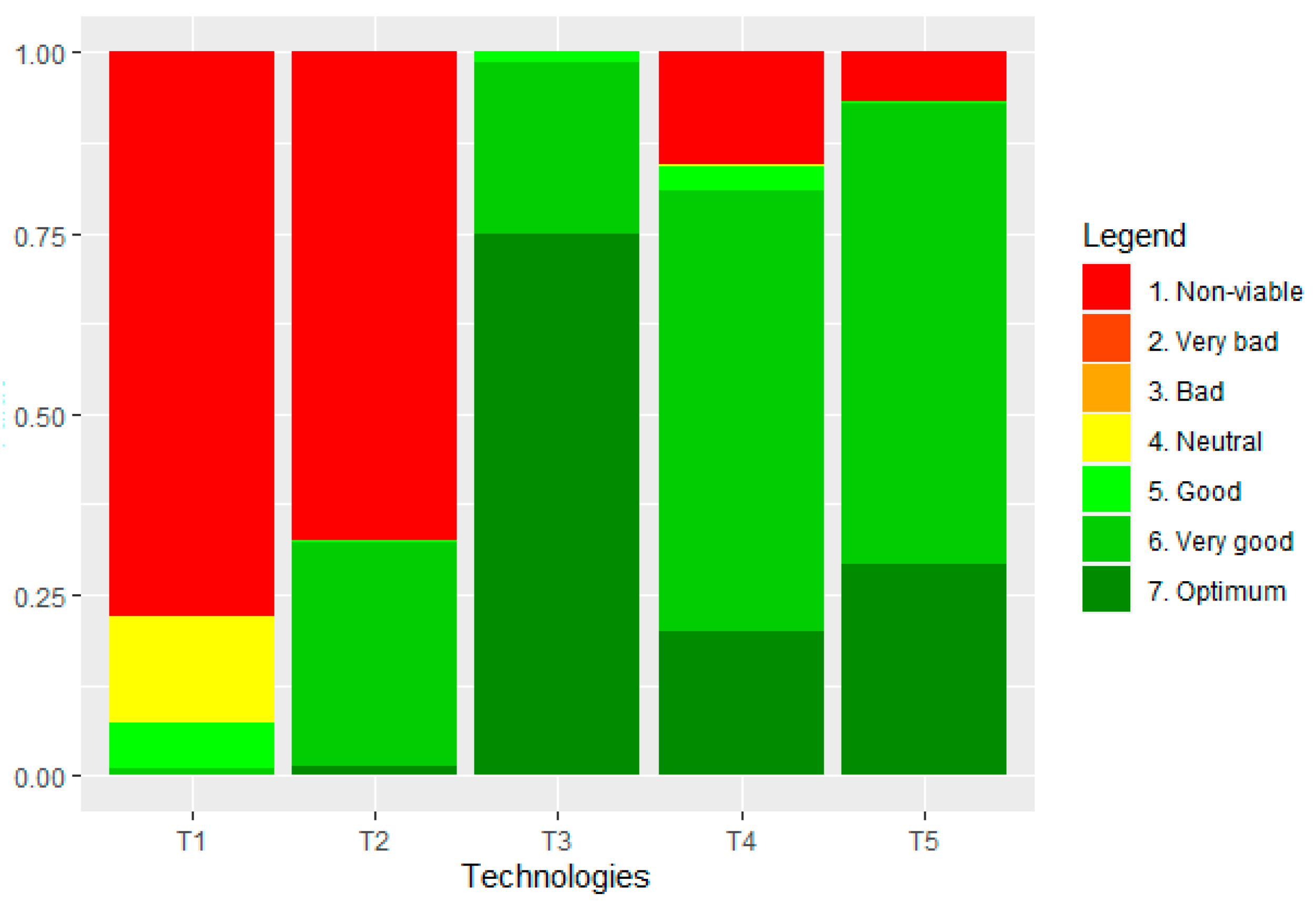
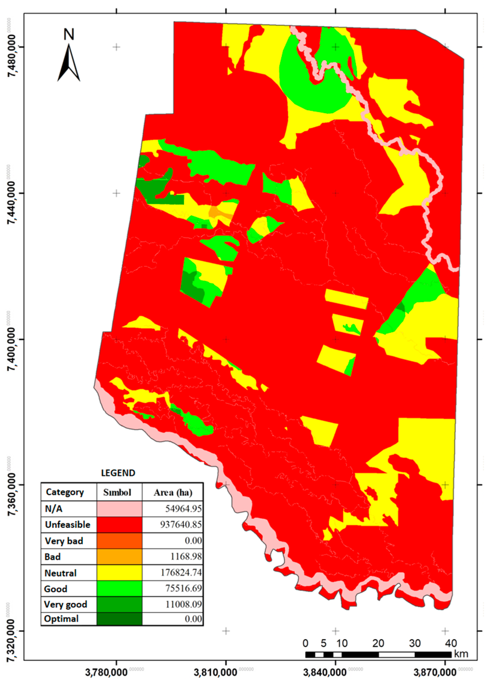
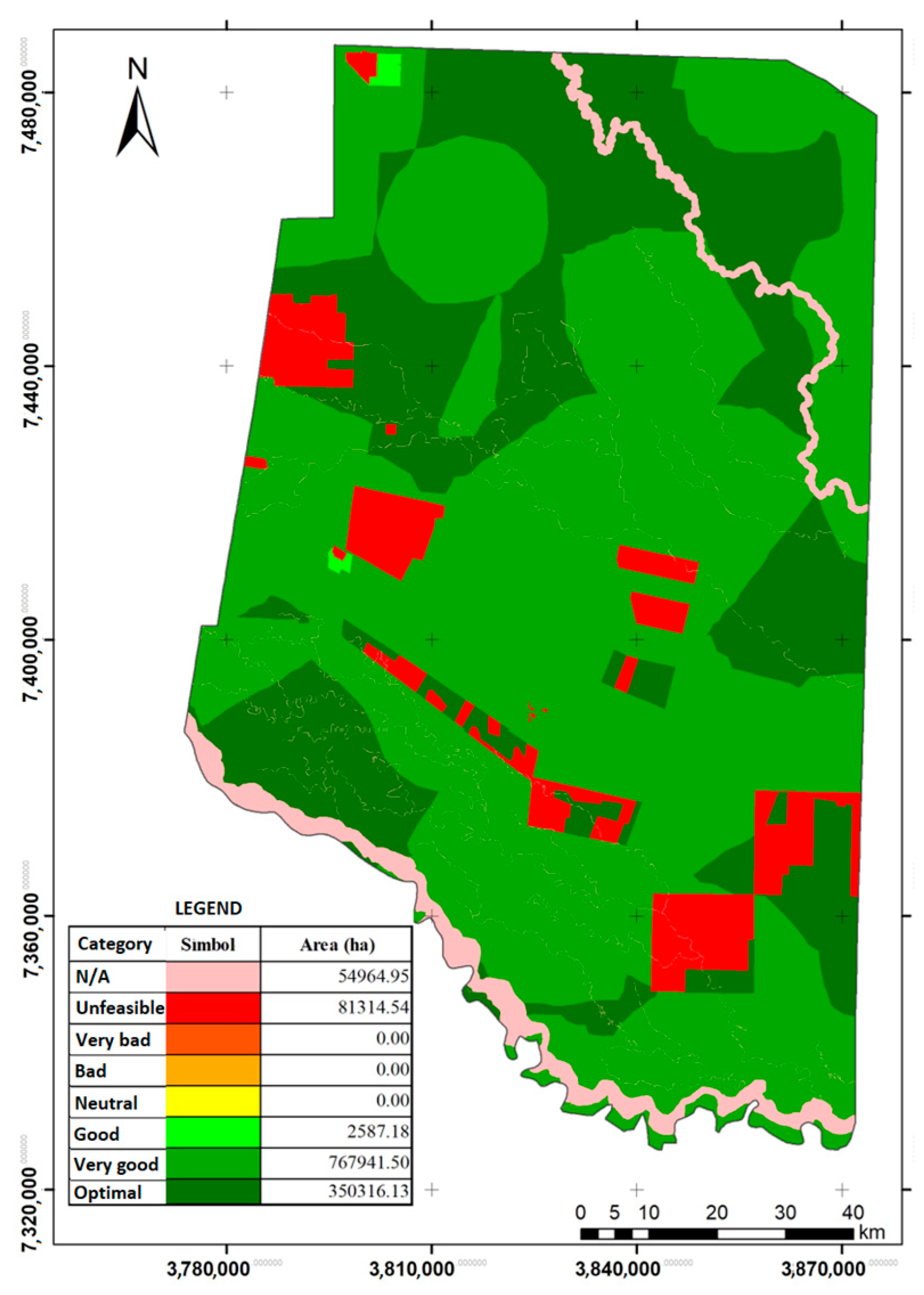
The results of the land evaluation are summarized in Figure 2 (maps included in Appendix C). The result for applying T1 gave a 78% of the area as nonviable, 14.71% as neutral, 6.24% as good and only 1% as very good. Thus, only a small extent of the study area is suitable for applying the T1 because this technology (precision agriculture) has high requirements for implementation.

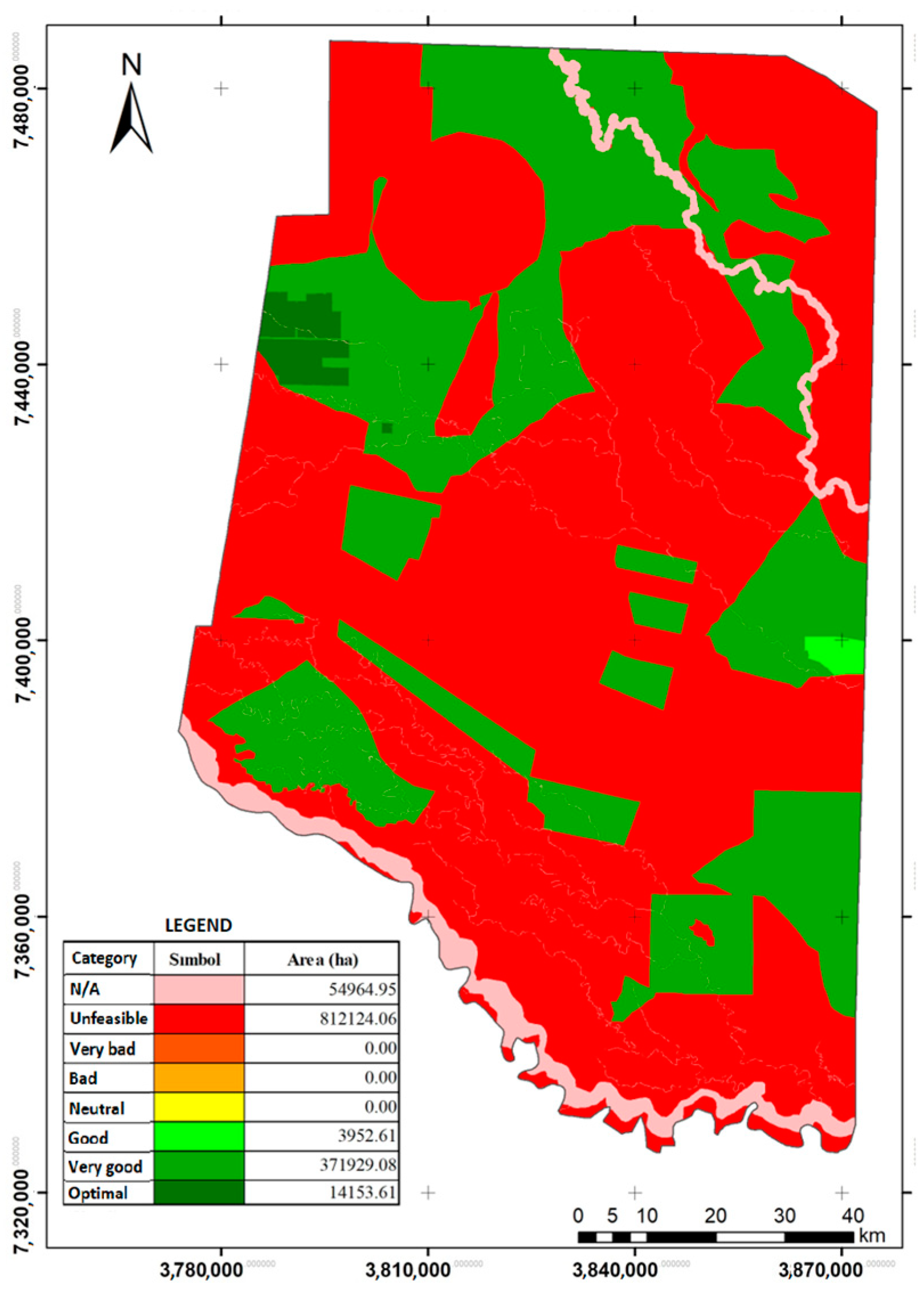
The outcome of the land evaluation for applying T2 includes 67.56% of the area as nonviable, 31% as very good, and only 1.18% as optimum. The suitable area for applying advanced livestock farming techniques is more extensive than for T1 (see Figure 2) but less than T3 to T5. T2 (forest with integrated livestock) requires an economic investment, technical planning, and studies but with not as high demands as those of T1.

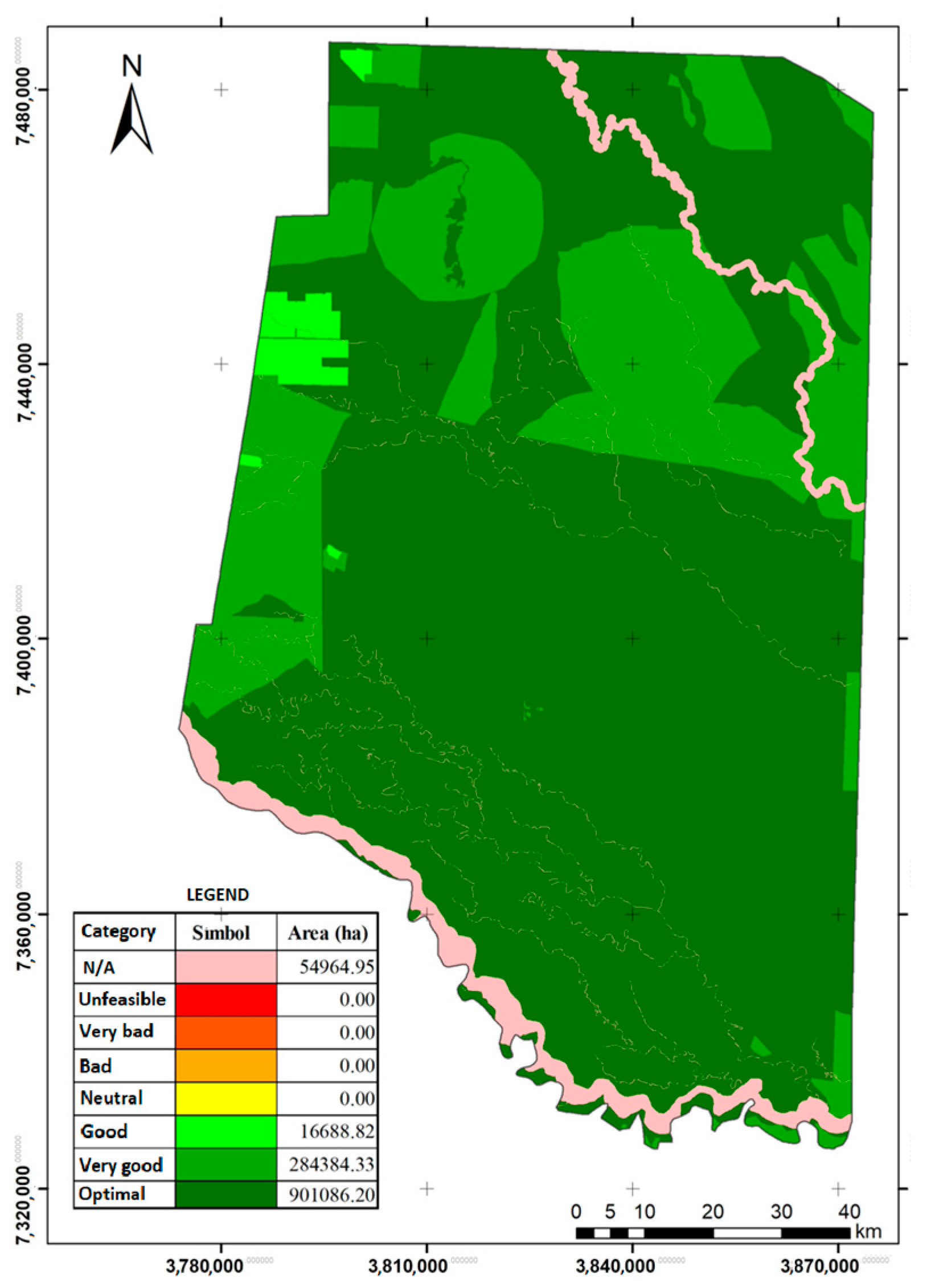
The outcome of the land evaluation for applying T3 includes 74.96% of the area as optimum, 23.66% as very good, and 1.39% as good. Most of the study area is suitable for applying this technique, because its main requirement is conserving the natural ecosystem to maintain its ecological services.

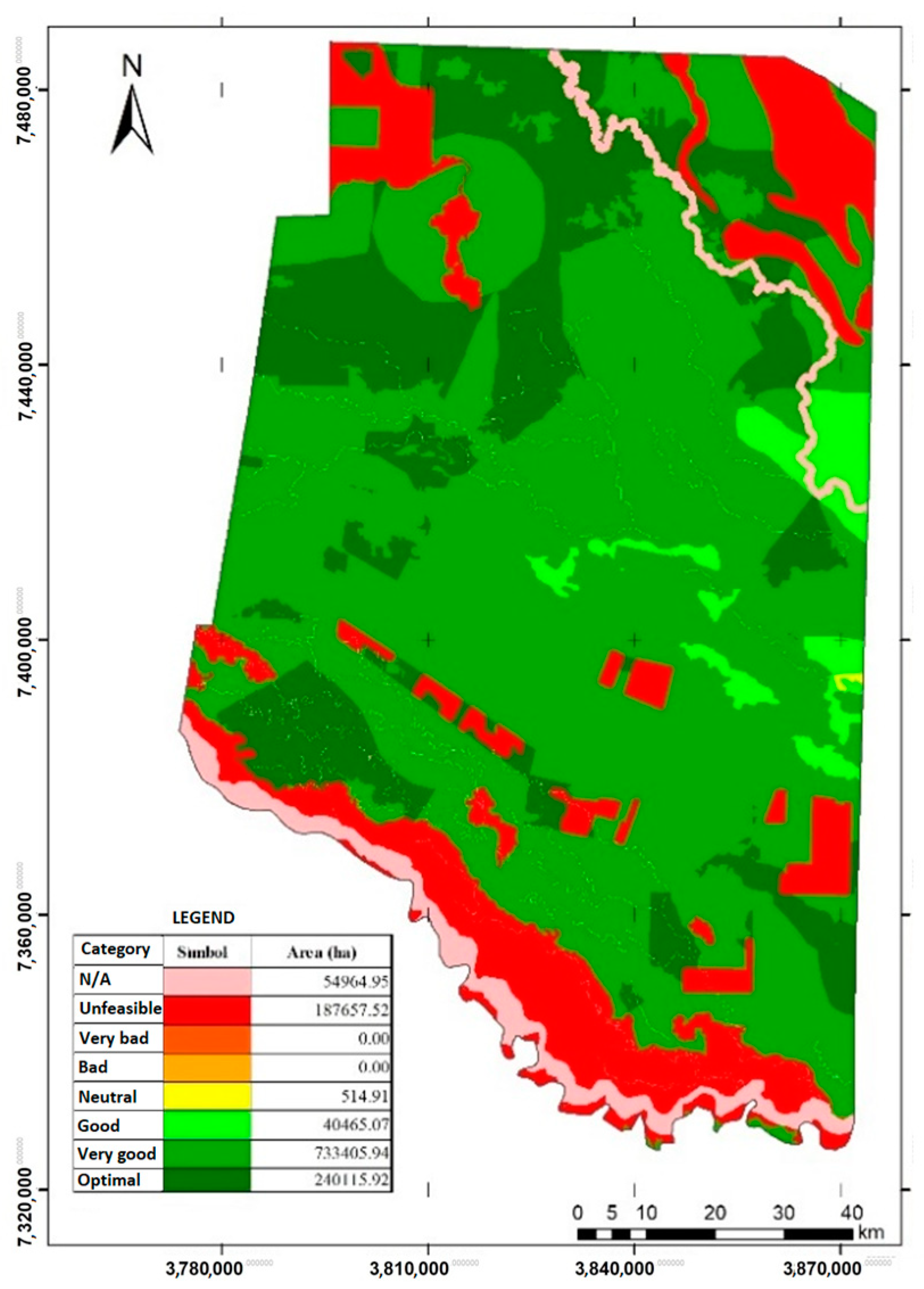
The results for applying T4 include 61.01% of the area as very good, 19.97% as optimum, and 15.61% as nonviable. This technique also has a large area suitable for application because, as a traditional Criollo livestock, it has fewer requirements than advanced livestock; the Criollo technique even allows browsing native grasslands and natural forests. Because of this unsustainable use [47], portfolio analysis of experts’ opinions indicates that no area percentage must be assigned to this technique, as we have seen previously.

The outcome for applying T5 includes 63.88% of the area as very good, 29.14% as optimum, and only 6.76% as nonviable. As in T4, the T5 has a large area suitable for application, because it has lower requirements for forest management traditionally and sustainably from timber, hunting, and gathering, as performed by Wichis.

As shown in Figure 2, the challenge for the Simplex method will be complex for techniques 1 and 2 because of its small suitable areas.

3.4. Land Distribution with Simplex Algorithm

As a result of the land evaluation, 57 combinations of the suitability categories for applying the five techniques were found, see

Table 6. Simplex method results for the optimal distribution of the five techniques (T1, T2, T3, T4, and T5) selection.

No.	Combination	Count	Area (Ha)	Zoning	Optimal Techniques Distribution
					T1	T2	T3	T4	T5
NA	0,0,0,0,0	163	54,964.95	N/A	0.00	0.00	0.00	0.00	0.00
1	0,0,4,7,0	11	2761.43	T3	0.00	0.00	2761.43	0.00	0.00
2	0,0,5,0,4	4	1241.12	T3	0.00	0.00	1241.12	0.00	0.00
	…
13	0,0,6,5,5	28	15,457.53	T3	0.00	0.00	15,457.53	0.00	0.00
14	0,0,6,6,0	1	246.79	T3	0.00	0.00	246.79	0.00	0.00
15	0,0,6,6,5	525	360,335.82	T3/T5	0.00	0.00	338,583.95	0.00	21,751.87
16	0,0,6,7,0	7	554.27	T3	0.00	0.00	554.27	0.00	0.00
17	0,5,6,5,6	3	3952.61	T5	0.00	0.00	0.00	0.00	3952.61
	…
31	4,6,6,0,6	8	2790.52	T2	0.00	2790.52	0.00	0.00	0.00
32	4,6,6,6,0	11	5427.79	T2	0.00	5427.79	0.00	0.00	0.00
33	4,6,6,6,6	50	38,956.42	T1/T2/T5	20,467.40	6878.97	0.00	0.00	11,610.05
34	4,6,6,7,0	1	30.38	T2	0.00	30.38	0.00	0.00	0.00
35	4,6,6,7,6	45	57,471.52	T2	0.00	57,471.52	0.00	0.00	0.00
	…
56	6,8,4,7,0	7	6827.24	T1	6827.24	0.00	0.00	0.00	0.00
57	6,8,6,6,0	1	176.98	T1	176.98	0.00	0.00	0.00	0.00
			1,202,159.35		106,992.18	267,480.46	472,328.41	0.00	355,358.30
					8.90%	22.25%	39.29%	0.00%	29.56%

. The Simplex method was executed on these 57 combinations to assign each to a technique from among the five possible, optimizing the area suitability and meeting the area objective derived from the portfolio analysis. The results show a perfect accommodation to the objective (T1 = 8.90%, T2 = 22.25%, T3 = 39.29%, T4 = 0.00%, and T5 = 29.56%), and it was found that each combination was only assigned to one optimal technique, except for the “0,0,6,6,5” and “4,6,6,6,6” combinations; these areas were divided among T3/T5 and T1/T2/T5, respectively (Table 6).

For these two cases with multiple technique assignation, the polygons with these combinations are distributed to achieve the required area for each technique. Each combination comprises many polygons, as shown in Table 6. The combinations “0,0,6,6,5” and “4,6,6,6,6” presented precise distributions (

Table 7. Techniques distribution among polygons of the “0,0,6,6,5” combination.

Techniques	Polygon Count	Area (Ha)
T3	506	338,583.95
T5	19	21,751.87
Total	525	360,335.82

and

Table 8. Techniques distribution among polygons of the “4,6,6,6,6” combination.

Techniques	Polygon Count	Area (Ha)
T1	27	20,467.40
T2	9	6878.97
T5	14	11,610.05
Total	50	38,956.42

), as there was no need to divide any polygon.

3.5. Geospacialization of the Optimal Distribution of the Five Techniques

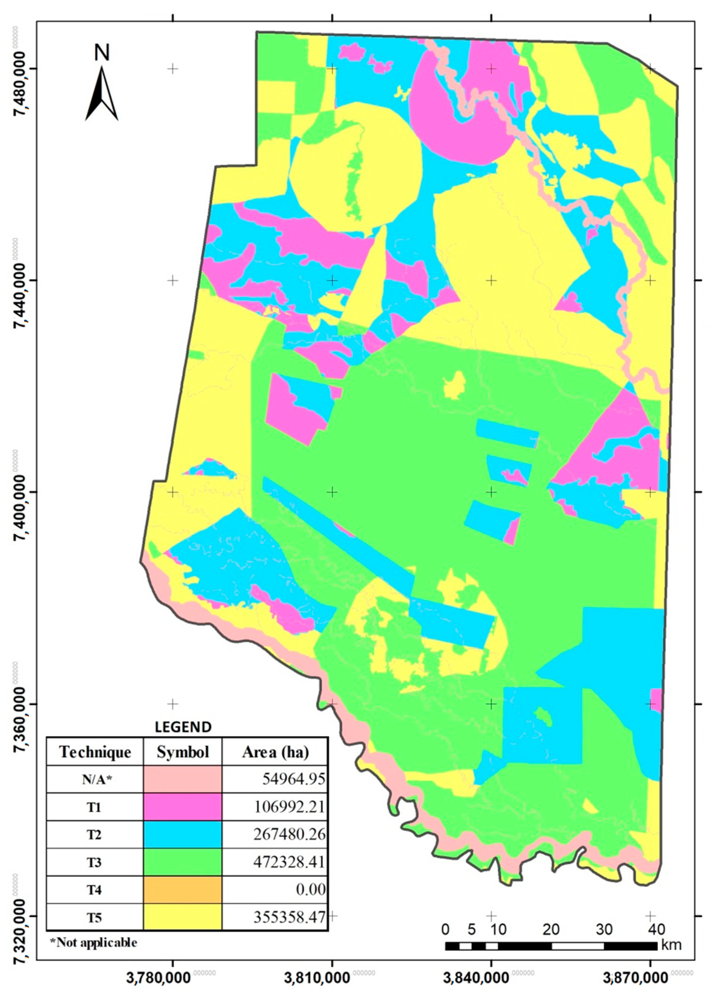
The optimal distribution of the five techniques obtained using the Simplex method in a GIS environment allows for plotting its distribution. As shown in the map (Figure 3), the techniques were distributed spatially, homogeneously, and in tight areas more extensive than a hectare, allowing for a straightforward application of the assigned technique. Also, it can be observed on the map that a few small portions of T1 appear to disperse but are constantly surrounded or in the neighborhood with T2, which makes it possible to integrate the management of these two techniques, which are related to the high level of technology and can be constituted as integral farms.

Considering the degree of optimization, 92% of the area is assigned to a technique with very good and optimal suitability, 6.5% of the area allocation has good suitability, 1.7% area has average suitability, and no area has bad or worst suitability. The good and average suitability correspond mainly to the precision agriculture technique, as it has more restrictive requirements than the others. Therefore, despite all of the constraints, allocating an area to appropriate uses with high suitability has been achieved.

4. Discussion

With the information available, the results can guide official land use or land ownership policies and technical assistance by national or local agricultural extension services.

It is highlighted that the lowest return (portfolio 1, Table 4) is obtained for the T5 technique linked to a high risk, i.e., the experts assign with a high discrepancy a limited socioeconomic value and implementation possibilities to the traditional activity of the Wichis.

The highest return (portfolio 15, Table 4) is generated for the T3 technique (payment for ecosystem services) with a medium–high risk, probably due to the difficulties in determining who will pay for ecosystem services and how. However, this technique will allow for the preservation of areas defined as nature reserves and to obtain extra income to complement the traditional activities of the Wichi and Criollos.

All portfolios agree not to assign a surface area to T4 because of its low profitability and high environmental impact. Although the land evaluation assigns a large amount of surface area to this technique as good or better (although little for optimal), the expert evaluation can detect its problems. This situation highlights the goodness of the developed method as opposed to the simple use adjustment to the land evaluation. Therefore, the population carrying out T4 could carry out T2 (forest with integrated livestock, which local INTA researchers have proposed) to continue their livestock production activity with higher income and sustainability. Given that this technique requires a high economic investment, technical planning, and prefeasibility studies in land use, the government and INTA should support the influential population to change orientation.

Another issue that can be addressed with the mapping results is the legalization of the ownership of the land currently owned by the state for the defined uses. Moreover, it would be possible to discuss the transfer of uses in lands legally and illegally occupied by Criollos and Wichis to activities that are not their traditional ones and how to provide the administrative, financial, and technical support for this transition.

Considering the groups of opinions detected among the experts has made it possible to choose the minimum risk portfolio versus the maximum Sharpe portfolio, the two most used solutions.

The results suggest an optimized goal of sustainable governance. However, it will not be possible to implement it without the commitment of the institutions and the occupants of the land, whatever their legal status. However, the developed method provides information for the negotiation process between the actors concerned.

The study’s limitations are mainly related to the underlying information, both in mapping the relevant variables and expert opinions. Information on more suitability-influencing variables and an improvement in the scale of the associated maps could ameliorate the allocation of surface areas. The information from the experts represents different local perspectives, and it was analyzed for consistency and groups were detected with different opinions, but this could be improved by expanding the sample size. Optimal use distribution mapping could also be generated for the differentiated analysis of each opinion group, and the variation in the results could be considered as a sensitivity analysis. However, the methodology developed will be able to produce solutions that are readjusted to better information or new constraints that are added.

5. Conclusions

A step-by-step methodology was developed that allowed us to perform complex land use planning. Based on expert opinions and environmental properties, we established an optimal cartographical distribution of the uses considered in the study area.

In addition to the two methodologies commonly used to solve these problems, land evaluation and GIS, two optimization methodologies were incorporated: Markowitz portfolio and Simplex linear programming. Markowitz’s portfolio model minimized the risk (disagreement among experts) and maximized return or profit (qualification of techniques by the experts). This model obtained the percentage of the study area that each of the five techniques defined must be managed. A Simplex method analysis combined with GIS was performed for the optimal allocation (maximizing land evaluation suitability) of homogeneous areas (GIS polygons with the same properties) to the five techniques in the percentage derived from experts’ opinion analysis.

The result achieved the objectives derived from the experts’ opinion on the techniques and the conditioning factors derived from the properties of the natural and social environment, making assignments in 92% of the area with very good or optimal suitability and producing a cartographic solution.

Improving and increasing the sources of information (i.e., cartographic and experts) or introducing other uses could improve the results. However, the stepwise methodology presented would also be applicable.

References

1. Schaumberg, H. Aboriginal conceptions of the forest in the soy era: Frontiers of deforestation in the Argentine Chaco. Curr. Opin. Environ. Sustain. 2020, 43, 99–105. [Google Scholar] [CrossRef]
2. Eagle, A.J.; Olander, L.P. Chapter Three—Greenhouse Gas Mitigation with Agricultural Land Management Activities in the United States—A Side-by-Side Comparison of Biophysical Potential. Adv. Agron. 2012, 115, 79–179. [Google Scholar]
3. Hasan, S.S.; Zhen, L.; Miah, M.G.; Ahamed, T.; Samie, A. Impact of land use change on ecosystem services: A review. Environ. Dev. 2020, 34, 100527. [Google Scholar] [CrossRef]
4. Arora, V.K.; Boer, G.J. Uncertainties in the 20th century carbon budget associated with land use change. Glob. Chang. Biol. 2010, 16, 3327–3348. [Google Scholar] [CrossRef]
5. Esteves, V.P.P.; Esteves, E.M.M.; Bungenstab, D.J.; Loebmann, D.G.D.S.W.; de Castro Victoria, D.; Vicente, L.E.; de Queiroz Fernandes Araújo, O.; do Rosário Vaz Morgado, C. Land use change (LUC) analysis and life cycle assessment (LCA) of Brazilian soybean biodiesel. Clean Technol. Environ. Policy 2016, 18, 1655–1673. [Google Scholar] [CrossRef]
6. Sirami, C.; Caplat, P.; Popy, S.; Clamens, A.; Arlettaz, R.; Jiguet, F.; Brotons, L.; Martin, J.-L. Impacts of global change on species distributions: Obstacles and solutions to integrate climate and land use. Glob. Ecol. Biogeogr. 2017, 26, 385–394. [Google Scholar] [CrossRef]
7. Biswas, A.; Pal, B.B. Application of fuzzy goal programming technique to land use planning in agricultural system. Omega 2005, 33, 391–398. [Google Scholar] [CrossRef]
8. Xie, H.; Lu, H. Impact of land fragmentation and non-agricultural labor supply on circulation of agricultural land management rights. Land Use Policy 2017, 68, 355–364. [Google Scholar] [CrossRef]
9. Mollet, J.A. Planning for Agricultural Development, 2nd ed.; Avebury: Aldershot, UK, 1990; ISBN 0566071428. [Google Scholar]
10. Sicular, T. Agricultural Planning and Pricing in the Post-Mao Period. China Q. 1988, 116, 671–705. [Google Scholar] [CrossRef]
11. Fischer, J.; Lindenmayer, D.B.; Manning, A.D. Biodiversity, ecosystem function, and resilience: Ten guiding principles for commodity production landscapes. Front. Ecol. Environ. 2006, 4, 80–86. [Google Scholar] [CrossRef]
12. Bai, L.; Liu, Y.; Wang, Q.; Chen, C. Improving portfolio performance of renewable energy stocks using robust portfolio approach: Evidence from China. Phys. A Stat. Mech. Appl. 2019, 533, 122059. [Google Scholar] [CrossRef]
13. Itoh, T.; Ishii, H.; Nanseki, T. A model of crop planning under uncertainty in agricultural management. Int. J. Prod. Econ. 2003, 81–82, 555–558. [Google Scholar] [CrossRef]
14. Way, R.; Lafond, F.; Lillo, F.; Panchenko, V.; Farmer, J.D. Wright meets Markowitz: How standard portfolio theory changes when assets are technologies following experience curves. J. Econ. Dyn. Control 2019, 101, 211–238. [Google Scholar] [CrossRef]
15. Zaidi, S.A.H.; Wei, Z.; Gedikli, A.; Zafar, M.W.; Hou, F.; Iftikhar, Y. The impact of globalization, natural resources abundance, and human capital on financial development: Evidence from thirty-one OECD countries. Resour. Policy 2019, 64, 101476. [Google Scholar] [CrossRef]
16. Recanati, F.; Guariso, G. An optimization model for the planning of agroecosystems: Trading o ff socio-economic feasibility and biodiversity. Ecol. Eng. 2018, 117, 194–204. [Google Scholar] [CrossRef]
17. Salles, M.; Gomes, E. Optimized Agricultural Planning of Sugarcane using Linear Programming. Rev. Investig. Operacional 2010, 31, 126–132. [Google Scholar]
18. Markowitz, H. Portfolio selection. J. Financ. 1952, 7, 77–91. [Google Scholar] [CrossRef]
19. Barkley, A.; Peterson, H.H.; Shroyer, J. Wheat variety selection to maximize returns and minimize risk: An application of portfolio theory. J. Agric. Appl. Econ. 2010, 42, 39–55. [Google Scholar] [CrossRef]
20. Knoke, T.; Paul, C.; Härtl, F.; Castro, L.M.; Calvas, B.; Hildebrandt, P. Optimizing agricultural land-use portfolios with scarce data—A non-stochastic model. Ecol. Econ. 2015, 120, 250–259. [Google Scholar] [CrossRef]
21. Paut, R.; Sabatier, R.; Tchamitchian, M. Reducing risk through crop diversification: An application of portfolio theory to diversified horticultural systems. Agric. Syst. 2019, 168, 123–130. [Google Scholar] [CrossRef]
22. Paut, R.; Sabatier, R.; Tchamitchian, M. Modelling crop diversification and association effects in agricultural systems. Agric. Ecosyst. Environ. 2020, 288, 106711. [Google Scholar] [CrossRef]
23. Wheeler, B.M.; Russell, J.R.M. Goal Programming and Agricultural Planning. J. Oper. Res. Soc. 1977, 28, 21–32. [Google Scholar] [CrossRef]
24. Xiang, W.-N. A GIS/MMP-Based Coordination Model and its Application to Distributed Environmental Planning. Environ. Plan. B Plan. Des. 1993, 20, 195–220. [Google Scholar] [CrossRef]
25. Chuvieco, E. Integration of linear programming and GIS for land-use modelling. Int. J. Geogr. Inf. Syst. 1993, 7, 71–83. [Google Scholar] [CrossRef]
26. Arthur, J.L.; Nalle, D.J. Clarification on the use of linear programming and GIS for land-use modelling. Int. J. Geogr. Inf. Sci. 1997, 11, 397–402. [Google Scholar] [CrossRef]
27. Gualotuña Parra, J.A.; Tarquis, A.M.; Grau Olivé, J.B.; Colombo Speroni, F.; Saa-Requejo, A. An analytical approach to assess the influence of expert panel answer on decision making: The case of sustainable land use in ribadavia banda norte, salta (Argentina). Sustainability 2021, 13, 6705. [Google Scholar] [CrossRef]
28. INTA. Cobertura del suelo de la República Argentina, año 2006–2009 (LCCS—FAO); INTA: Buenos Aires, Argentina, 2009. [Google Scholar]
29. INTA. Adecuación a un Sistema de Información Geográfica del estudio “Los Suelos del NOA (Salta y Jujuy), Nadir A.—Chafatinos T. 1990” EEA; INTA: Salta, Argentina, 2009; ISBN 9789872505080. [Google Scholar]
30. Ippolito, T.A.; Herrick, J.E.; Dossa, E.L.; Garba, M.; Ouattara, M.; Singh, U.; Stewart, Z.P.; Prasad, P.V.V.; Oumarou, I.A.; Neff, J.C. A Comparison of Approaches to Regional Land-Use Capability Analysis for Agricultural Land-Planning. Land 2021, 10, 458. [Google Scholar] [CrossRef]
31. Secretaría de Ambiente de la provincia de Salta Mapa “Ordenamiento Territorial de Bosques Nativos (OTBN) 2009—Provincia de Salta” escala 1:500.000. Available online: https://directory.spatineo.com/service/47641/ (accessed on 1 December 2022).
32. Congreso de la Nación Argentina. Presupuestos Mínimos de Protección Ambiental de los Bosques Nativos; Ley 26.331. 2007. Available online: http://servicios.infoleg.gob.ar/infolegInternet/anexos/135000-139999/136125/norma.htm (accessed on 1 December 2022).
33. Schmidt, M. Native Forests Territorial Management: Definitions and discussions in the province of Salta. Aproximaciones Teóricas Medio Nat. Transform. Territ. 2010, 1, 27. [Google Scholar]
34. Instituto Nacional de Asuntos Indígenas. Distribución Geográfica de los Pueblos Originarios Según Comunidades Registradas en el Ámbito Nacional y/o Provincial. 2022. Available online: https://www.argentina.gob.ar/derechoshumanos/inai/mapa (accessed on 1 December 2022).
35. Venencia, C.D.; Correa, J.J.; del Val, V.; Buliubasich, C.; Seghezzo, L. Conflictos de tenencia de la tierra y sustentabilidad del uso del territorio del Chaco salteño. Energías Renov. Medio Ambient. 2012, 30, 29–35. [Google Scholar]
36. Belmonte, S.; de las Mercedes López, E.; de los Ángeles García, M. Identificación de áreas prioritarias para la gestión del agua en el Chaco salteño, Argentina. Agua Territ. Water Landsc. 2021, 17, 7–32. [Google Scholar] [CrossRef]
37. Claro, S.A. Mapa de Cobertura 3G y 4G en Argentina. Available online: https://www.claro.com.ar/personas/planes-prepago-pospago/cobertura (accessed on 1 December 2022).
38. Ayers, R.S.; Westcot, D.W. Water Quality for Agriculture; California, EE.UU; Food and Agriculture Organization of the United Nations: Rome, Italy, 1985; Volume 29, ISBN 9251022631. [Google Scholar]
39. Costa, J.L.; Aparicio, V.C. Quality assessment of irrigation water under a combination of rain and irrigation. Agric. Water Manag. 2015, 159, 299–306. [Google Scholar] [CrossRef]
40. Markowitz, H.M. Portfolio theory: As I still see it. Annu. Rev. Financ. Econ. 2010, 2, 1–23. [Google Scholar] [CrossRef]
41. Batcheller, J.K. Automating geospatial metadata generation—An integrated data management and documentation approach. Comput. Geosci. 2008, 34, 387–398. [Google Scholar] [CrossRef]
42. Elias, B. Pedestrian Navigation-Creating a tailored geodatabase for routing. In Proceedings of the 2007 4th Workshop on Positioning, Navigation and Communication, Hannover, Germany, 22 March 2007; IEEE: Manhattan, NY, USA, 2007; pp. 41–47. [Google Scholar]
43. Rossiter, D.G. A theoretical framework for land evaluation. Geoderma 1996, 72, 165–190. [Google Scholar] [CrossRef]
44. Valverde-Arias, O.; Garrido, A.; Valencia, J.L.; Tarquis, A.M. Using geographical information system to generate a drought risk map for rice cultivation: Case study in Babahoyo canton (Ecuador). Biosyst. Eng. 2018, 168, 26–41. [Google Scholar] [CrossRef]
45. Gualotuña Parra, J.A. Elección de Técnicas Productivas y Zonas de Implementación Para el Desarrollo Sostenible en el Municipio de Rivadavia Banda Norte, Salta, Argentina. Doctoral Thesis, Universidad Politécnica de Madrid, Madrid, Spain, 2022. [Google Scholar]
46. Bekanov, K.K.; Safarov, E.; Prenov, S.; Yusupov, B. Optimization of Agricultural Land Use in Chimbay District of the Republic of Karakalpakstan Using GIS Technologies. Int. J. Geoinform. 2022, 18, 27–36. [Google Scholar] [CrossRef]
47. Camardelli, M.C.; Caruso, H.; de Bianchi, S.P.; Pérez, D.; Miranda, S. Evaluación de cambios tempranos en la calidad de los suelos relacionados con el carbono en tierras ganaderas del Chaco semiárido salteño. Rev. Científica Agropecu. 2005, 9, 173–179. [Google Scholar]
Figure 1. Schematic representation of the GIS methodology.
Sustainability 15 11050 g001
Figure 2. Results of the suitability evaluation classes (surface% for each category) for applying technologies.
Sustainability 15 11050 g002
Figure 3. Optimal distribution of the five techniques according to the expert criteria using the Simplex method.
Sustainability 15 11050 g003