How Urban Morphology Relates to the Urban Heat Island Effect: A Multi-Indicator Study

Abstract

Urban morphology quantitatively expresses a city’s spatial structure, internal relationships, and physical form. It has advantages for predicting urban growth and analyzing the current state of cities in the literature. A comprehensive study on the complex relationships between urban morphology and urban heat island intensity (UHII) is of great importance for mitigating the urban heat island (UHI) effect for megacities. This study models urban morphological indicators in fine resolution based on three aspects: building morphology, ecological infrastructure, and human activities. The model accurately captures UHII by employing the definition of UHI effects. The relationship between urban morphology and UHII was further examined using extreme gradient boosting (XGBoost) and Shapley additive explanations (SHAP). By taking central Beijing, China as study area, major findings include the following: (1) Significant daytime UHI effects were observed within the research area, particularly during the summer months, when it appears to be most severe. More than 90% of the region experiences varying degrees of the UHI effects. (2) UHI is significantly correlated with both 2D and 3D urban morphological indicators. Low sky view factor (SVF) and high SVF tend to mitigate UHI, whereas moderate SVF tends to aggravate UHI. (3) In densely populated areas, tall trees may be more effective than other forms of vegetation at mitigating UHI. Based on the aforementioned findings, this article suggests that urban morphology optimization should focus on seasonality, spatial specificity, and indicator specificity for megacities in urban design and spatial planning aimed at mitigating UHI.

1. Introduction

In recent years, cities have become essential living spaces for over half of the world’s population, and the continuous growth of urban populations has resulted in significant transformations in urban morphology [1]. Humans colonize the biosphere by replacing natural land surfaces with impermeable built environments, resulting in anthropogenic emissions, such as heat and pollution, and the destruction of vegetation could otherwise absorb these emissions [2]. Consequently, urban areas exhibit higher air and surface temperatures compared to outlying rural regions, known as the urban heat island (UHI) phenomenon [3]. With the ongoing expansion of cities, the UHI effect has been intensifying, leading to various detrimental impacts on society, including increased energy consumption [4], aggravated pollution [5], and adverse effects on people’s health conditions and status of wellbeing [6]. Therefore, it is imperative to address this issue urgently and gain a clear understanding of the factors influencing UHI in order to effectively mitigate its harmful effects.

Research has shown that the UHI effect is influenced by multiple factors, including climatic components, urban morphology, land surface characteristics, and human activities [7]. While previous studies have primarily focused on climatic component and land surface characteristics, urban morphology actually plays a crucial role in the formation and growth of the UHI effect [8]. Differing from climatic components and land surface characteristics, urban morphology encompasses various aspects such as urban structure types, landscape patterns, and settlement density, which are key factors in the formation and development of the UHI effect [9]. Numerous studies have demonstrated that urban morphology substantially affects surface temperature [10]. However, due to the multiple quantitative indicators associated with urban morphology, which can describe the spatial structure, internal relationships, and landform characteristics of cities from different perspectives, the main objective of this study is to comprehensively establish the correlation between 2D and 3D indicators at a fine scale and the UHI effect.

At the macroscale of cities, some progress has been made in the study of the relationship between urban morphology and UHI. Using spatial autocorrelation analysis, geographically weighted regression, and other techniques, researchers have analyzed the relationship between urban landscape and the UHI effect [11]. This field of study emphasizes the importance of land use changes, impervious surfaces, vegetation, and water bodies in contributing to the UHI effect [12,13,14]. However, the role of urban morphology, such as building height and building density, is often overlooked in many cases. The influence of urban morphology on the UHI effect is particularly prominent at the microscale. As a result, several studies have proposed that urban morphological features at the microscale, such as building density and layout, can significantly impact the urban heat island effect. Nevertheless, most indicators are based on 2D analyses, while it has been demonstrated that 3D spatial morphology represents a crucial characteristic of urbanization.

In a 3D urban context, some researchers have examined the relationship between urban morphology and the UHI effect [15]. The majority of experimental studies utilize medium-to-high-resolution remote sensing images in conjunction with digital surface models to extract building form characteristics [16]. Nonetheless, this approach is incapable of acquiring accurate details regarding the contour and altitude of individual constructions. In contemporary times, the swift advancement of remote sensing technology has led to the increasing prevalence of 3D geographic information data, which encompass building story heights and building outlines. These data provide effective support for extracting large-scale fine-grained urban 3D spatial form indicators, such as sky view factor and building density [17,18]. Consequently, using 3D geographic information data for building feature extraction has become a widely discussed method. The majority of researchers have only calculated the Pearson correlation coefficient between the landscape and UHI effect, concluding that the majority of landscape indicators are significantly correlated, but lacking a detailed analysis of the effect of each morphology indicator on the UHI effect [19]. Simultaneously, certain researchers have only considered the impact of building space while disregarding the mutual influence between various land cover types [20], resulting in the insufficient explanatory power of morphology indicators for the UHI effect. Moreover, there is a divergence of opinions regarding the effectiveness of 3D urban morphological indicators in influencing UHI compared to 2D indicators [18,21].

Traditional regression analysis models, such as multiple linear regression [22] and polynomial regression [23], are based on predefined linear or nonlinear relationships and still have advantages in certain specific scenarios. However, their ability to handle complex relationships is limited. On the other hand, machine learning models have the capability to automatically learn complex relationships from data, enabling them to better fit complex real-world problems and nonlinear relationships [24]. Random forests, XGBoost, support vector machines, and artificial neural networks are widely used models in current research [25]. Although machine learning models have been proved effective in classification and regression, it still remains challenging to understand the interrelationships between the factors with these ‘black box’ models [26]. At the same time, traditional regression analysis methods are inadequate to support in-depth analysis of the correlation between various urban morphological indicators and the UHI effect [27]. To address these issues, we have introduced an interpretable modeling approach, known as the Shapley additive explanations (SHAP) method. The SHAP model is one of the methods based on the framework of explainable artificial intelligence (XAI) [28], which is designed to increase the interpretability and explainability of AI models [29,30]. In addition, we have also considered the comprehensive impact of different urban land cover types, such as buildings, water bodies, and vegetation, on the relationship between urban morphology and UHI.

The purpose of this study is to use multisource remote sensing data to construct 2D/3D urban morphology models and emerging SHAP interpretable models to achieve quantitative modeling of urban morphology expression, and to investigate the correlation between urban morphology and the UHI effect. Specific objectives are (1) to introduce multi-indicators to characterize 2D/3D urban morphology; (2) to explore the relationship between urban morphology and UHI during different seasons, including its stability and variations; (3) to investigate the impact of various urban morphologies on the UHI effect. It is important to note that although this study investigates the variations of the seasonal UHI effect, the adverse impacts of UHI on the environment and human health are particularly pronounced during summer daytime [31]. Therefore, the focus of this study lies primarily on summer daytime conditions. As part of this work, the following research questions are addressed: (1) How do different types of indicators impact on UHI? (2) Are the effects of indicators on UHI consistent across different seasons?

The relationship between urban morphology and the UHI effect is comprehensively explored by this study, which can also offer advice for urban planners and policymakers on how to enhance the urban thermal environment during the summer days through rational landscape planning and urban management.

2. Materials and Methods

2.1. Urban Morphology Indicators and Data Preparation

The present research institute focused on urban climate has a plethora of indicators about urban morphology, thereby posing a challenge in ascertaining the typical and representative indicator type. Drawing upon earlier definitions of the urban spatial form [32,33,34], and by the research objectives of this investigation, a total of eight indicators were identified to characterize urban morphology. The building form indicators were all derived from building vector data, including diversity of building shapes (DBS), floor area ratio (FAR), sky view factor (SVF), and building height (HIGH). The indicators normalized difference built-up index (NDBI), modified normalized difference water index (MNDWI), and normalized difference vegetation index (NDVI) were calculated using Landsat 8 satellite imagery data. The population density (PD) indicator was derived from population raster data. These indicators collectively encompass various aspects of building form, ecological infrastructure, and human activity.

Table 1. Urban morphology indicators.

Type	Name	Description	Calculation
2D building form indicators	Diversity of building shapes (DBS)	The diversity of building shapes in the area	$D=1-\frac{{\displaystyle \sum }n\left(n-1\right)}{N\left(n-1\right)}$
	Floor area ratio (FAR)	The density of the horizontal distribution of buildings	$R=\frac{Q}{S}$
	Normalized difference built-up index (NDBI)	Building and impermeable surface coverage	$\mathrm{NDBI}=\left(\mathrm{SWIR}-\mathrm{NIR}\right)/\left(\mathrm{SWIR}+\mathrm{NIR}\right)$
3D building form indicators	Sky view factor (SVF)	The extent to which the sky is blocked by buildings	$SVF=1-\frac{{{\displaystyle \sum }}_{i=0}^n\sin {\gamma }_i}{n}$
	Building height (HIGH)	The average height of buildings in the area	$HIGH=L\ast H$
Ecological infrastructure	Normalized difference vegetation index (NDVI)	Growth, abundance, and coverage of vegetation	$\mathrm{NDVI}=\left(\mathrm{NIR}-\mathrm{Red}\right)/\left(\mathrm{NIR}+\mathrm{Red}\right)$
	Modified normalized difference water index (MNDWI)	Coverage of water bodies	$\mathrm{MNWDI}=\left(\mathrm{Green}-\mathrm{SWIR}\right)/\left(\mathrm{Green}+\mathrm{SWIR}\right)$
Human activities	Population density (PD)	The density of population in the area	/

Notes: $D$ is the diversity index, $N$ is the total number of individuals, $n$ is the number of individuals. $R$ is the volume ratio, $Q$ is the total area of the space unit building, $S$ is the area of the plot. n = 360, ${\gamma }_i$ is the direction of the observer’s line of sight. $L$ is the number of storeys, $H$ is the height of the storey. $\mathrm{NIR}$ indicates the reflectance of the infrared band, $\mathrm{Red}$ indicates the reflectance of the red band in the visible band, $\mathrm{Green}$ indicates the visible green band. $\mathrm{SWIR}$ indicates the reflectance of the shortwave infrared band.

enumerates the classification and explication of each indicator.

Table 2. Experimental data introduction.

Data Type	Resolution	Time	Use
Landsat 8 satellite imagery	Thermal infrared band 30 m Multispectral band 100 m	17 December 2017 (Winter) 27 June 2018 (Summer) 8 April 2018 (Spring) 17 October 2018 (Autumn)	Surface temperature inversion
Building vector	-	2018	Calculation of morphological indicators
Population raster	100 m	2018	Population density calculations
Resources Satellite Three imagery	2.1 m	2018	Auxiliary data
Nighttime light data	30 m	2015	Auxiliary data
Impervious surface data	30 m	2015	Auxiliary data

presents the spatial resolution of each dataset. To ensure consistency of scale for regression analysis, a 500 m × 500 m grid was used for sampling in ArcMap 10.2, taking into account differences in data types and resolution.

The present study used Landsat 8 satellite imagery, building vector data, Resource 3 satellite imagery data, and population data as the primary sources of information. Table 2 provides a comprehensive account of the resolution, acquisition time, and utilization of each dataset. The selection of Landsat 8 satellite images was based on choosing four images with cloud cover less than 10% during the period from December 2017 to October 2018. The preprocessing of data typically encompasses several key steps, such as radiometric calibration, atmospheric correction, and the cropping of vector data to focus on the study area.

2.2. Urban Heat Island Intensity Calculation

Urban heat island intensity (UHII) is a significant metric utilized for evaluating the urban thermal environment. Its magnitude is intricately linked to factors such as urban morphology, land utilization, and population density. Hence, the examination of alterations and determinants of UHII holds significant pragmatic implications. This study utilized preprocessed Landsat 8 satellite image data and used the single-window algorithm [35] to perform land surface temperature inversion.

Table 3. Background field temperature.

Date	Values
Winter—December 2017	2.07 °C
Spring—April 2018	23.12 °C
Summer—June 2018	36.33 °C
Autumn—October 2018	17.57 °C

displays the inversion outcomes of land surface temperature for the months of December 2017 and June, April, and October 2018.

The concept of UHII pertains to the disparity between the mean temperature in the primary urban zone and the mean temperature in the neighboring suburban or rural regions. This metric serves as an indicator of the strength of the UHI effect [36]. Thus, the equation for computing UHII can be expressed as:

$$UHI{I}_G=T_G-T_{rural} G=1, 2\dots n$$

(1)

The calculation for $T_{rural}$ is as follows:

$$T_{rural}={\displaystyle \sum }_{i=1}^k{T}_i/k$$

(2)

$T_G$ is the surface temperature value, $T_{rural}$ is the background field temperature, $k$ is the total number of surface temperature values in the background temperature field region.

The present investigation utilized a methodology for selecting the urban background temperature field that was derived from prior scholarly works [37,38]. In this paper, we used the method proposed by Li [39] to detect urban growth and extract complete urban region (Figure 1). This method utilizes two valuable remote sensing data sources: nighttime light data and impervious surface data. The nighttime light data were obtained from the NCEI National Centers for Environmental Information, while the impervious surface data were acquired from Liu’s team [40]. The area outside the urban boundary with the same area as the urban area was determined as the urban background temperature field, and the average land surface temperature within this area was regarded as the urban background temperature [41].

The background field area is shown in Figure 1.

2.3. Interpreting Machine Learning Models

2.3.1. XGBoost Regression

XGBoost is a decision tree-based machine learning algorithm [42] that is widely used for classification and regression tasks. Its core formulation can be expressed as follows:

$$F\left(y\right)=\phi \left(X_i\right)={\displaystyle \sum }_{k=1}^k{f}_k\left(X_i\right)$$

(3)

$F\left(y\right)$ is the predicted output of the model, $X_i$ denotes the input variable, $f_k$ denotes the $k$th weak evaluation function, $i$ denotes the mean sample.

The XGBoost used involves the utilization of gradient boosting for the iterative training of a sequence of decision trees, followed by the application of weighted averaging to produce the ultimate predictions [43]. The XGBoost algorithm has been found to have an advantage over other machine learning methods, such as random forests and support vector machines. This advantage lies in its ability to enhance prediction accuracy while simultaneously reducing the computational cost. This is achieved by amalgamating weak regression trees into a robust model, whereby each tree endeavors to rectify residuals in predictions made by its predecessors [44]. Furthermore, the XGBoost algorithm utilizes a technique for identifying splits that is sensitive to sparsity during the training of sparse data. This approach is particularly advantageous when working with data that have low sampling rates, such as remotely sensed data. Based on the research objectives and data sources of this study, it can be concluded that the XGBoost model is the most appropriate option for conducting regression analysis.

2.3.2. Shapley Additive Explanations (SHAP) Method

The significance of model interpretability is on the rise with the increasing prevalence of machine learning in diverse domains. The opaqueness inherent in conventional machine learning techniques renders the comprehension and interpretation of such models arduous. Consequently, the investigation of techniques and instruments for interpreting models has emerged as a prevalent domain of scholarly inquiry. The primary emphasis in machine learning is typically on the precision and capacity for generalization of the model. However, it is important to note that the prediction and decision-making mechanisms of the model are also of critical importance [45].

Therefore, to comprehend the XGBoost regression model and its impact on UHII through various indicators, the present study presents a novel approach to the interpretation of machine learning models, specifically the SHAP method. Compared with many other interpreting approaches such as the single-tree approximation method, decision rule extraction, refining method, feature importance, and saliency mask methods [46], the SHAP method offers more consistent and locally accurate attribution values that are individualized for each prediction. The SHAP methodology is founded upon the principle of Shapley values, which serve to elucidate the influence of individual features on the resultant output of a given model. The Shapley value, as initially introduced by Lloyd Shapley [47] in the field of game theory, serves to evaluate the individual contributions made by each participant towards achieving a win in a given game. The Shapley value is a technique employed in the field of machine learning to determine the individual contribution of each feature toward the model prediction. Through the computation of the Shapley value for individual features, it is possible to derive a hierarchy of feature importance concerning the model’s predictions, thereby enhancing our comprehension of the model’s predictive outcomes.

Furthermore, the SHAP methodology produces both a comprehensive and a specific interpretation for each instance by amalgamating the contribution of each feature’s shape value with its actual value. The overarching interpretation pertains to the model’s performance on the complete dataset, whereas the specific interpretation pertains to the model’s performance on individual samples. The aforementioned interpretations can facilitate comprehension of the decision-making mechanism of the model, offer indications for enhancing the model’s efficacy, and augment the dependability and explicability of the model’s predictions. The present investigation examines the relationship between the SHAP values and the degree of impact, as well as the directionality of changes, associated with individual indicators on the intensity of the UHI effect. The calculation of SHAP values is accomplished through the utilization of the formula as denoted by reference [48].

$${Ø}_j={\displaystyle \sum }_{\mathrm{S}\subseteq \left\{{\mathrm{x}}_{1,\dots ,{\mathrm{x}}_{\mathrm{p}}}\right\}\backslash \left\{{\mathrm{x}}_{\mathrm{j}}\right\}}\frac{\left|\mathrm{S}\right|!\left(\mathrm{p}-\left|\mathrm{S}\right|-1\right)!}{\mathrm{p}!}({\mathrm{f}}_{\mathrm{x}}\left(\mathrm{SU}\left\{x_j\right\}\right)-f_x\left(S\right))$$

(4)

${Ø}_j$ represents the contribution of the jth feature, x is the vector of feature values of the instance to be explained, p is the number of features, $f_x\left(S\right)$ represents the prediction of the feature values in a subset S.

The SHAP algorithm is available at https://github.com/slundberg/shap (accessed on 6 December 2022) for information on specific calculation methods.

3. Results

3.1. Experimental Area

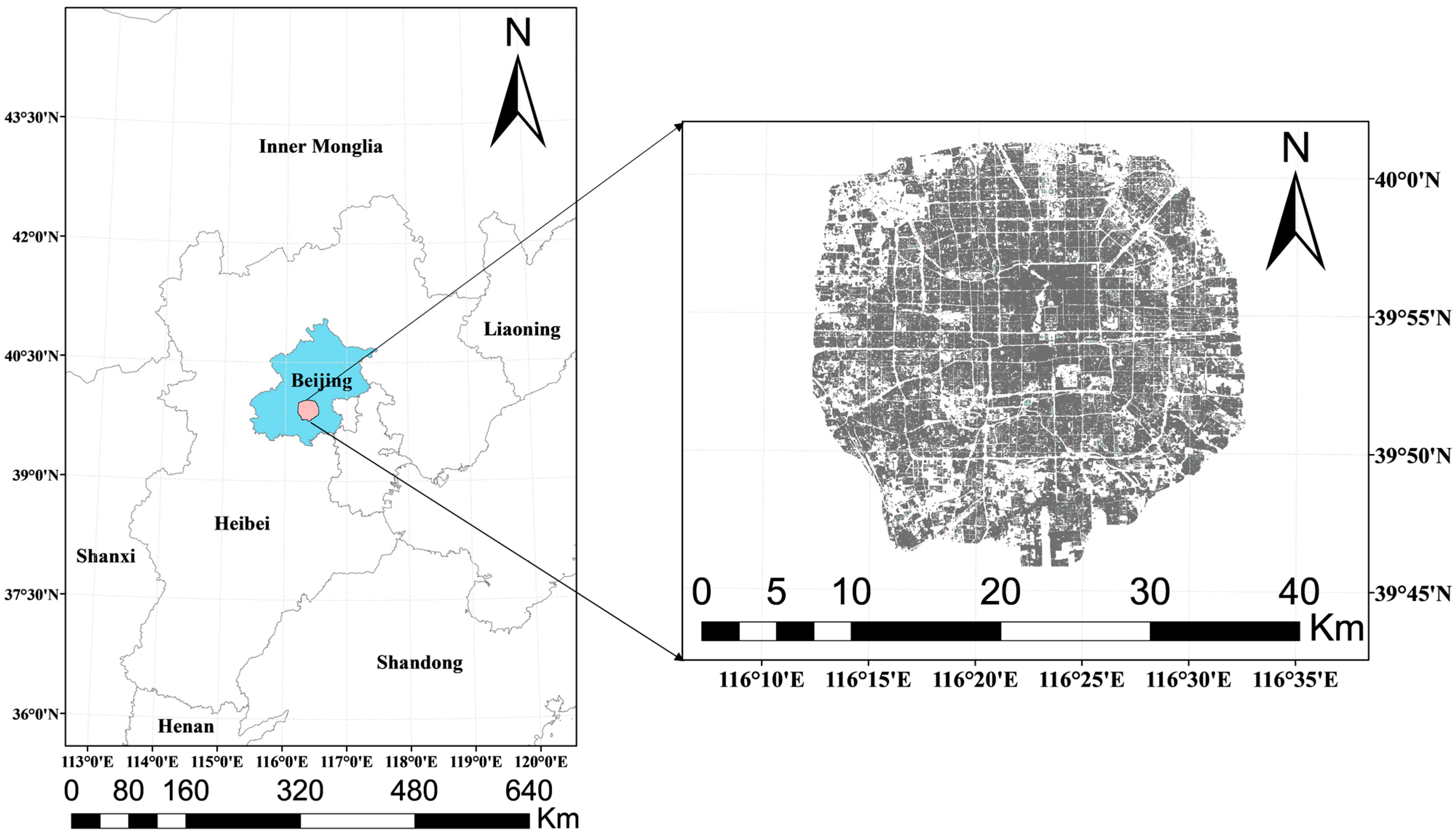
The city of Beijing is situated in the northern region of China, with its central point located at a longitude of 116°20′ East and a latitude of 39°56′ North. It is surrounded by the regions of Inner Mongolia, Hebei, and Tianjin. Beijing, being the capital of China, serves as a hub for political affairs, cultural activities, international communication, and scientific and technological advancements, encompassing a multitude of urban functions. The climate of Beijing is characterized as a warm temperate semihumid and semiarid monsoon climate, exhibiting significant fluctuations in temperature across the seasons [49]. During the winter season, spanning from December to February, the mean temperature typically hovers around −10 °C, with the possibility of the temperature dropping to subzero levels of below −20 °C. During the summer season, which spans from June to August, the mean temperature typically hovers around 25 °C, while the maximum temperature can exceed 40 °C. The city of Beijing experiences a concentrated amount of precipitation during the summer season, with an estimated average annual precipitation of approximately 630 mm. By the conclusion of 2022, it is projected that Beijing will harbor a populace of 21.843 million and attain a regional Gross Domestic Product of CNY 416.09 billion [50]. The swift growth of Beijing’s populace, infrastructure, and economy has significantly influenced the city’s urban morphology [51]. Simultaneously, the expeditious proliferation of the metropolis has resulted in numerous environmental challenges, particularly the effect of the UHI. Beijing is deemed as a suitable city for this research based on its climatic and socioeconomic attributes. Due to the large overall area of Beijing and the presence of mountainous suburban areas, the city has expanded in a central pattern of urban development. Therefore, this study mainly focuses on the area within the Fifth Ring Road, which has an approximate area of 667 square kilometers. Figure 2 displays the geographical region under investigation.

3.2. Distribution of UHII and Correlation of Multiple Indicators

This study utilized Landsat 8 remote sensing images within the Fifth Ring Road area of Beijing for four distinct periods spanning from 2017 to 2018. The surface temperature was inferred through implementation of the single-window algorithm, and the UHII was calculated using the UHI definition. The UHII calculation outcomes were classified into six categories using the Jenks natural break method [52] inversion results. These categories include non-heat island regions (<0 °C), low-intensity heat island regions (0–0.5 °C), medium-intensity heat island regions (0.5–2 °C), subintensity heat island regions (2–3.5 °C), high-intensity heat island regions (3.5–6.5 °C), and very-high-intensity heat island regions (>6.5 °C).

The spatial distribution of UHII exhibits significant seasonal variations, as illustrated in Figure 3a. A distinct “strong west-east and strong south-north” pattern characterizes the UHII distribution. During winter, the high-intensity and very-high-intensity heat island areas are primarily concentrated within the Second Ring Road and southwest of the Fourth to Fifth Ring Roads. Utilizing the ArcMap raster calculator, the quantification of image elements was computed, revealing that the corresponding area constitutes approximately 30% of the aggregate. By contrast, during the summer season, the UHI effect exhibits a more severe manifestation within the Fifth Ring Road. A majority of the regions within this area, approximately 90%, demonstrate distinct levels of the UHI effect, which appear to cluster in a discernible pattern. The findings illustrated in Figure 3b,c indicate that regions with high-intensity heat islands are predominantly situated in residential zones characterized by compact constructions. Conversely, non-heat island areas are primarily situated in blue-green spaces that are encircled by water bodies and vegetation. This means that water plays the most obvious role in the dissipation of heat in Beijing. However, it is worth noting that regions with a prevalence of vegetation also exhibit reduced UHII. It is an indisputable fact that regions characterized by a high concentration of buildings exhibit elevated UHII levels. Chapter 4 will provide a more comprehensive analysis.

The objective of this research was to examine the correlation between the intensity of UHII and the multi-indicator. Initially, a Pearson correlation coefficient analysis was performed to evaluate the linearity of the association between the variables and to quantify the extent of correlation between the two variables before executing a regression analysis. The correlation coefficient is a numerical measure that varies from −1 to 1. A coefficient of 1 denotes a complete positive correlation, a coefficient of −1 denotes a complete negative correlation, and a coefficient of 0 denotes no correlation. The objective of this analysis is to ascertain the potential correlation between UHII and the multi-indicator. This will aid in the selection of appropriate independent variables for subsequent regression analyses.

Table 4. Pearson’s correlation between multi-indicator and UHII.

UHII	FAR	DBS	HIGH	SVF	PD	NDVI	NDBI	MNDWI
Spring	0.418 **	0.398 **	−0.426 **	−0.237 **	0.092 **	−0.125 **	0.339 **	−0.179 **
Summer	0.410 **	0.426 **	−0.298 **	−0.222 **	0.005	−0.364 **	0.339 **	−0.072 **
Autumn	0.378 **	0.338 **	−0.384 **	−0.213 **	0.064 **	−0.115 **	0.215 **	−0.209 **
Winter	0.289 **	0.355 **	−0.348 **	−0.173 **	0.008	0.245 **	0.171 **	−0.321 **

** Correlation is significant at the 0.01 level (2-tailed).

displays Pearson’s correlation coefficients computed for the multi-indicator about UHII. The correlation coefficients for the building indicators remain consistent across all four seasons, both positively and negatively. However, it is noteworthy that certain building indicators exhibit inverse correlations. FAR and DBS exhibit positive correlations throughout all seasons, whereas HIGH and SVF demonstrate negative correlations throughout all seasons. The correlation coefficients exhibit significant variation across the diverse indicators, with the FAR indicator maintaining a value of approximately 0.4 and the SVF indicator approximately −0.2. The study found that there were significant negative correlations between vegetation and water bodies across all seasons, except winter, where vegetation indicators displayed positive correlations. While the majority of indicators were observed to have a significant impact on UHII throughout all seasons, except the PD indicator, none of the indicators were deemed adequate in independently elucidating the spatial dispersion of UHII.

3.3. XGBoost Regression between Multi-Indicator and UHII

To further investigate the impact of various indicators on UHII, an XGBoost regression model was used to analyze multiple indicators, as presented in

Table 5. The percentage of explained variance of UHII with different variable groups (under the significance level of 0.05).

Variable Group	Percentage of Explained Variance of UHII
	Spring	Summer	Autumn	Winter
2D building indicators	48.10%	45.60%	39.00%	38.10%
3D building indicators	35.10%	28.90%	30.70%	28.50%
all building indicators	56.30%	57.50%	49.10%	47.20%
ecological infrastructure indicators	29.50%	23.20%	30.50%	31.00%
all multi-indicators	60.60%	61.20%	53.70%	54.50%

Note: the higher the percentage, the darker the shade of red.

. These five sets of independent variables were analyzed separately using XGBoost regression models to examine the relative prominence of each indicator during specific seasons. The indicators were categorized into five groups of independent variables: 2D building indicators, 3D building indicators, all building indicators, ecological infrastructure indicators, and all multi-indicators. As for the regression performance metric, it is not feasible to compare feature importance across different groups due to its metric-specific nature. We chose explained variance (R²) to offer a clearer explanation for performance variations among model groups. Because UHII varies significantly across seasons, a sampling grid of 500 m by 500 m was used, and distinct XGBoost regression models were developed for each season. Table 5 shows that the models created for the 3D indicators had a lower R², whereas the R² of all spatial 2D indicators was enhanced in comparison to the 3D indicators across all four seasons. Summer showed a significant difference of 16.7%. The 2D indicators predict UHII better than the 3D indicators. However, it is important to note that the 2D indicators do not provide a comprehensive representation of the building indicators. This improvement is because the building metrics models perform significantly better than their 2D counterparts. Specifically, during the autumn season, the R² value increased by 10.1%. Blue and green spaces are important in urban areas. Including the ecoinfrastructure index may improve the ability to predict UHII by an average increase of approximately 5% compared to the building model in isolation. These findings indicate that using various indicators can enhance the ability to predict UHII.

3.4. Contributions from Multi-Indicators Based on SHAP Summary Plots

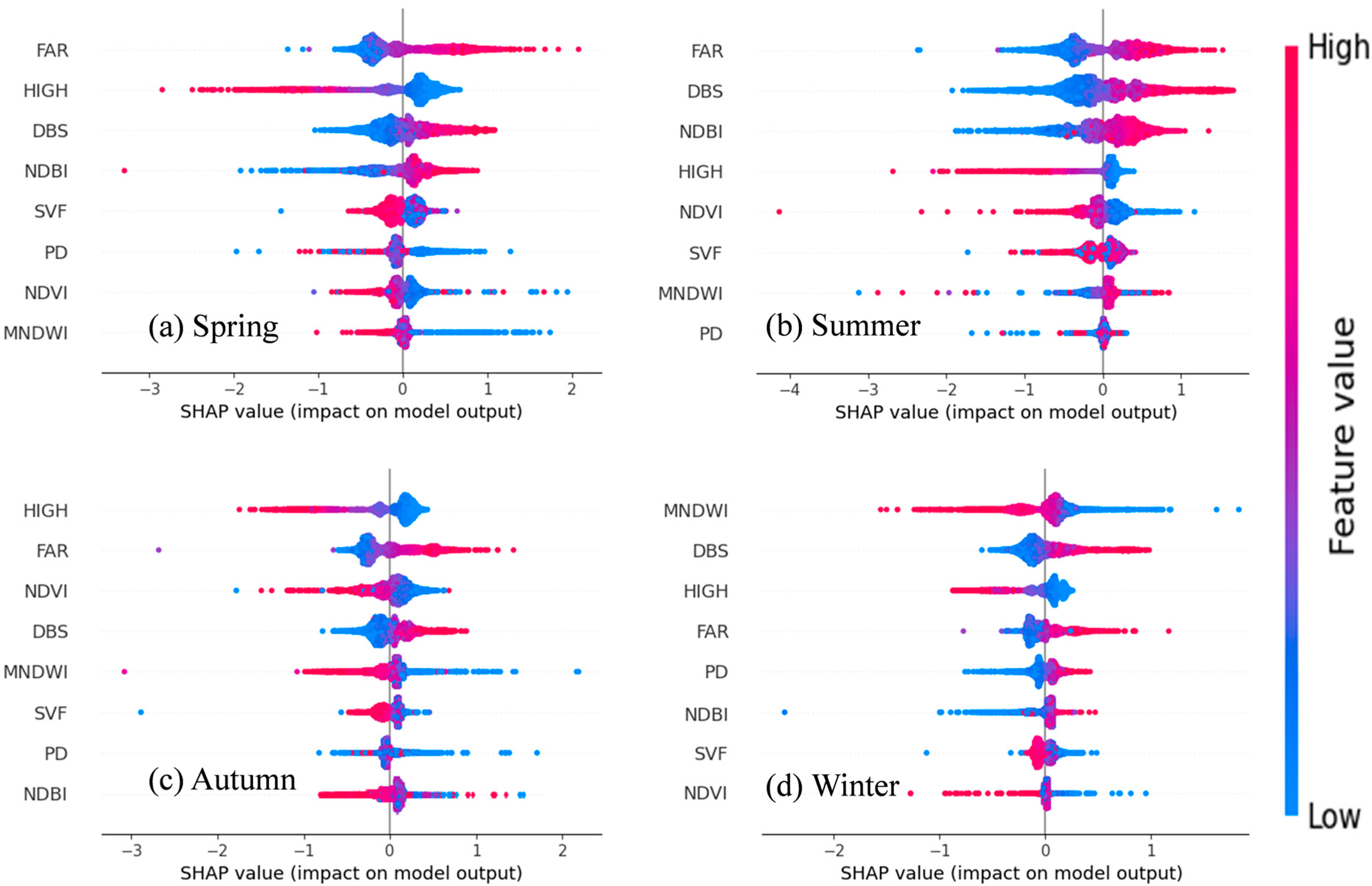
Although XGBoost regression performs well in modeling complex nonlinear relationships, it does not provide a comprehensive account of the contribution of each independent variable to the dependent variable. To improve understanding of the model’s forecasts and explain the function of the independent variables in the model, this investigation introduces the SHAP interpretable technique. The SHAP approach can explain the impact of individual 3D terrain metrics on changes in UHII. Figure 4 presents the SHAP values for various metrics. The arrangement of metrics along the y-axis is based on their respective contributions to UHII in each regression model, with the topmost metric having the highest contribution and the bottommost metric having the lowest contribution. The chromatic scheme used in the representation of the indicator values shows that red and blue hues correspond to the magnitude of the values, with the transition from blue to red indicating an increase in magnitude and a shift from negative to positive values, respectively. The horizontal axis of the chart displays the dispersion of SHAP values for the image components of the fishnet grid.

Based on the data presented in Figure 4a,b, it can be observed that the UHII experiences a significant impact from the FAR (positive) during the spring and midsummer seasons. The intensity of spatial development pertains to the level of infrastructure, such as buildings, present within an urban area. Typically, an elevated spatial development intensity within an urban area implies a greater number of structures, thereby resulting in an escalation of the UHI effect [53]. The findings suggest that a decrease in the degree of spatial development can have a notable impact on mitigating the UHI effect within urbanized regions. Based on the findings presented in Figure 4c,d, it can be inferred that the two primary factors that impact UHII during varying seasons are HIGH (negative) and MNDWI (negative). The MNDWI indicator exhibits a noteworthy capacity to alleviate the heat island effect across all seasons, albeit exerting a substantial impact on UHII solely during winter. Water bodies have the potential to impact UHII by modulating the temperature of the surrounding environment via the absorption and release of heat [54]. Additionally, water bodies can facilitate air convection, whereby cooler air from the water body is transported into the surrounding area, resulting in a cooling effect [55]. The parameter of building height, when altered, has a notable impact on the intensity of the UHI effect, as indicated by the HIGH (negative) value. The rationale behind this phenomenon is that the increased height of buildings leads to a heightened flow of ambient air, thereby exerting a greater impact on the alteration of ambient temperature and consequent exacerbation of the heat island effect [56].

It is noteworthy that based on the empirical findings illustrated in Figure 4d, the NDBI metric exhibits a moderating influence on the UHI effect during the winter season. However, the extent of this moderating effect is not statistically significant. There is a conjecture that the reason for this phenomenon could be attributed to the dissipation of absorbed heat by impermeable surfaces in the city, which occurs at a faster rate during winter. Consequently, areas of the city with a greater concentration of impermeable surfaces exhibit relatively lower temperatures. The empirical findings indicate that DBS (positive) exerts a more significant influence on the intensity of heat island across all seasons, as opposed to the NDBI indicator, as illustrated in Figure 4a–d. Furthermore, the DBS indicator’s contribution to the UHII ranks among the top four in all four seasons, indicating its relative immunity to seasonal variations. The regions exhibiting elevated DBS values indicate a greater intricacy of architectural design and a concomitant rise in the ratio of surface area to volume of the buildings, thereby augmenting the absorption and reflection potential of the building surface. According to research, complex buildings in urban areas tend to absorb solar radiation and heat more efficiently than simpler buildings, leading to an overall increase in temperature within the city [57]. Furthermore, it is noteworthy that the intricacy of building structures may have an impact on the air circulation in urban areas. It is plausible that buildings with more intricate designs could hinder airflow, leading to an increase in heat transfer between buildings and a decrease in the exchange of heat between the building mass and its surroundings [58]. Consequently, it is plausible that intricate architectural structures with multifaceted configurations could exacerbate the UHI effect in comparison to those with a uniform shape.

Based on the empirical findings depicted in Figure 4, it can be inferred that the NDVI (negative) exhibits a robust ameliorating impact on the UHI effect throughout all seasons, whereby an increase in vegetation coverage corresponds to a decrease in the intensity of the UHI effect [59]. The reason for this phenomenon is that vegetation can assimilate solar radiation and utilize it for photosynthesis, leading to a decrease in the amount of solar radiation that reaches the ground directly. Furthermore, it is worth noting that the transpiration process of vegetation has the potential to decrease the surrounding temperature. The experimental results presented in Section 3.2 indicate that PD (positive) is only pertinent during the spring and autumn seasons. Furthermore, the findings in this section, as illustrated in Figure 4, demonstrate that PD has a lesser impact on the UHII in comparison to the other indicators. This finding suggests that alterations in population density do not constitute the primary determinant of the UHI effect in densely populated regions. Section 4.1 provides a continuation of the comprehensive analysis of the individual indicators.

Consequently, the strategic implementation of vegetation and trees possessing high space-filling capacity across the three dimensions of the urban landscape is crucial in addressing the issue of the UHI effect. Likewise, within metropolitan areas, the erection of architecturally unobstructed skyscrapers plays a more significant role in mitigating UHII than level impermeable terrains.

4. Discussion

4.1. Influences of Multi-Indicators on UHII

The comprehension of the UHI effect heavily relies on the energy balance equation, which has gained significant use in UHI research [43,51,60]. The energy balance equation is a mathematical expression that characterizes the equilibrium between the amount of energy that enters and exits a given system. The UHI effect can be analyzed and evaluated through the utilization of this method, which also considers the factors that contribute to its formation. The energy balance equation serves as the fundamental framework for devising effective strategies to mitigate and alleviate the UHI effect. The equation for energy balance was initially introduced by Oke [61]:

$$Q^{*}+Q_F=Q_H+Q_E+\mathsf{\Delta }{Q}_S+\mathsf{\Delta }{Q}_A$$

(5)

where $Q^{*}$ represents the net all-wave radiation, $Q_F$ represents artificial heat, $Q_H$ represents the sensible heat flux, $Q_E$ represents the latent heat flux density, $\mathsf{\Delta }{Q}_S$ represents the heat storage flux, $\mathsf{\Delta }{Q}_A$ represents the advective heat flux.

The surface heat storage flux is the main source and sink term in the energy balance equation of the urban subsurface, and plays an important role in the redistribution of surface energy. The difference in energy balance due to the different subsurface characteristics of urban and suburban areas is the basis for the heat island effect [51]. The surface in urban centers consists mainly of buildings, vegetation, and water bodies, while suburban areas consist mainly of natural surfaces, agricultural land, and woodland. Therefore, to solve the UHI effect problem, the contribution of buildings, water bodies, and vegetation to the heat island effect needs to be sorted out. This section focuses on the contribution of each morphological indicator to UHII based on the best regression model selected by the XGBoost algorithm, using SHAP dependency plots.

4.1.1. The Influence of Building in 2D/3D Space

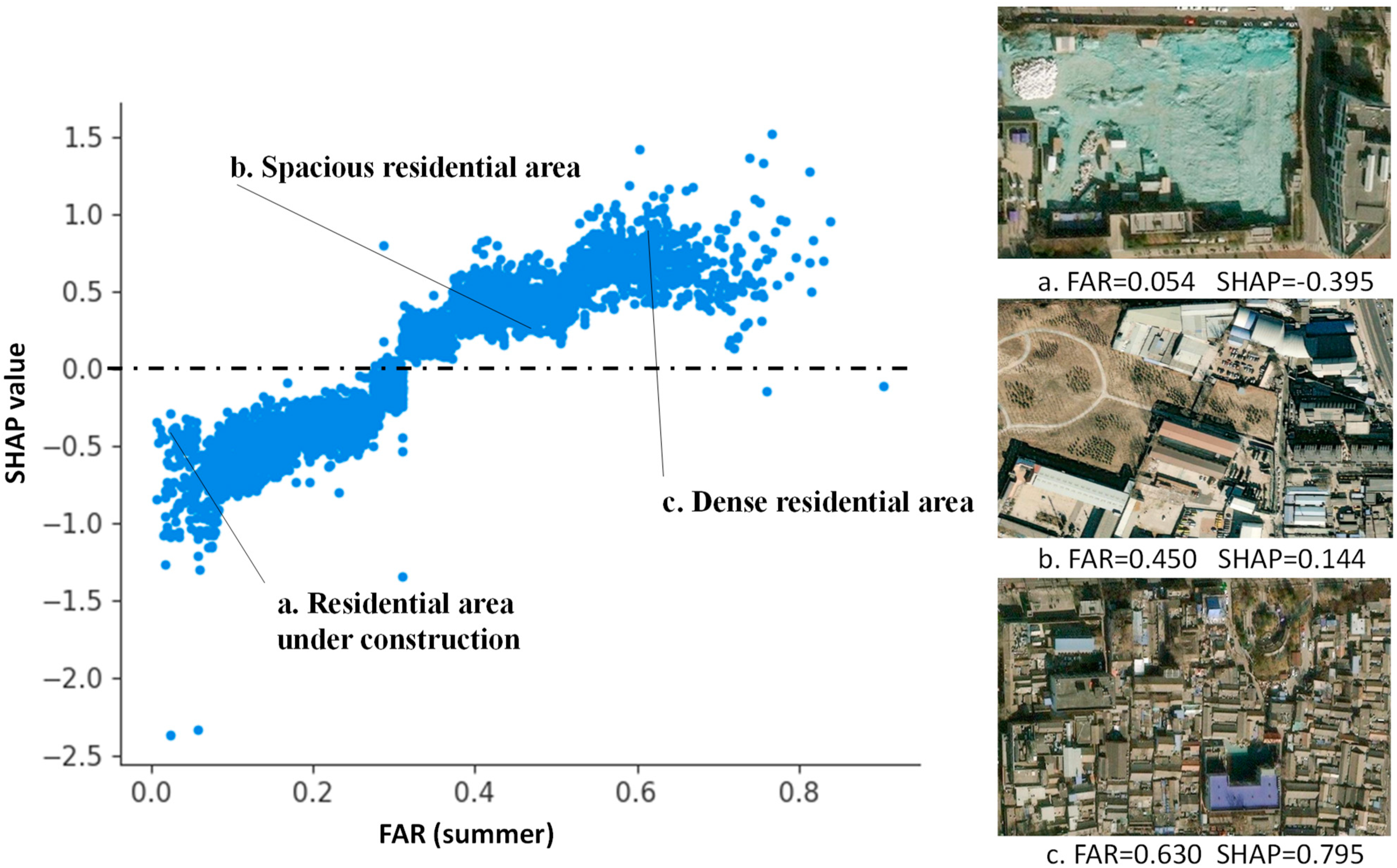
The impact of buildings on UHI is multifaceted and contingent upon the interplay of various factors. The utilization of urban 3D morphology knowledge to facilitate intelligent urban planning holds the potential to offer a viable resolution in addressing the unavoidable UHI effect that arises as a result of urbanization [43]. The FAR indicator is frequently employed to characterize the land use status and level of urbanization in various geographical areas, such as cities, regions, or countries, by measuring the density and coverage of buildings developed within a particular land area or spatial extent [34]. Figure 5 demonstrates that the SHAP value exhibits a positive correlation with the FAR value, eventually plateauing as the FAR value approaches 0.5. Based on the observations made in Figure 5a–c, it is evident that regions characterized by low FAR exhibit a moderating influence on the UHI effect. Conversely, areas with high-density development tend to exacerbate the UHI effect. The impact of building density on local-scale surface temperature, air temperature, and UHII is a significant consideration [62]. The arrangement of buildings frequently assumes a crucial and fundamental function in the emergence of the UHI effect within a given locality. Once the degree of building development in a particular region is determined, there exists the limited potential for modifying the UHI effect through alterations to the building structure [63].

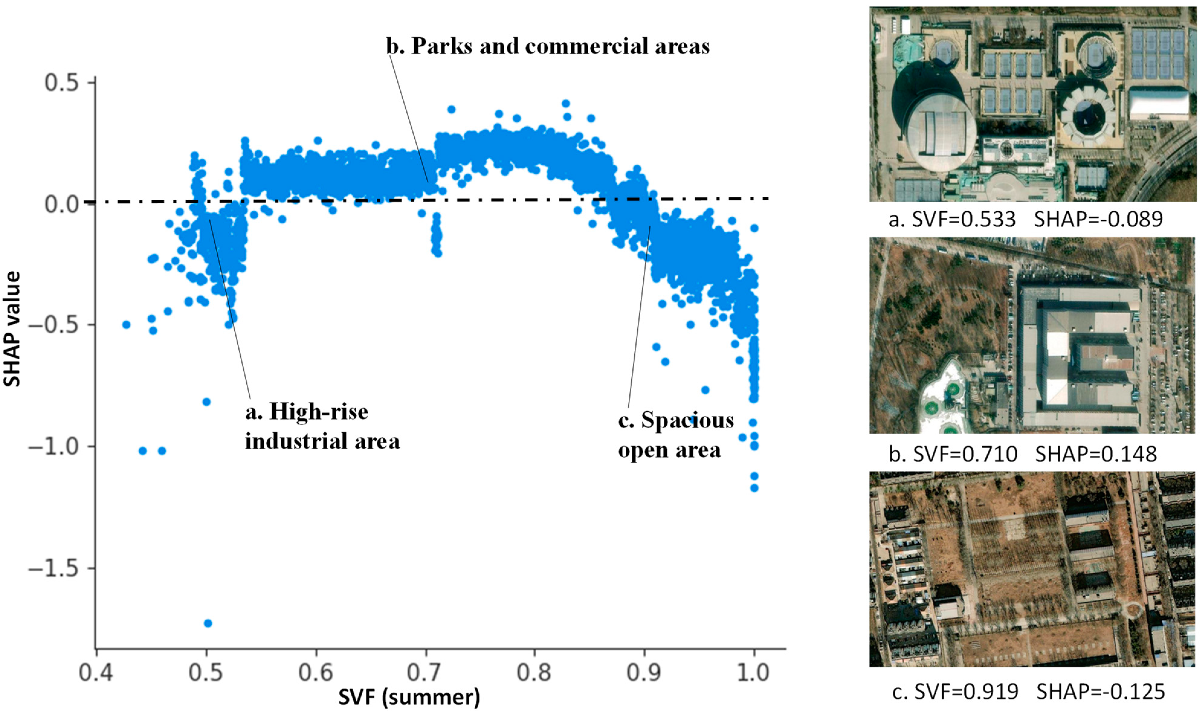
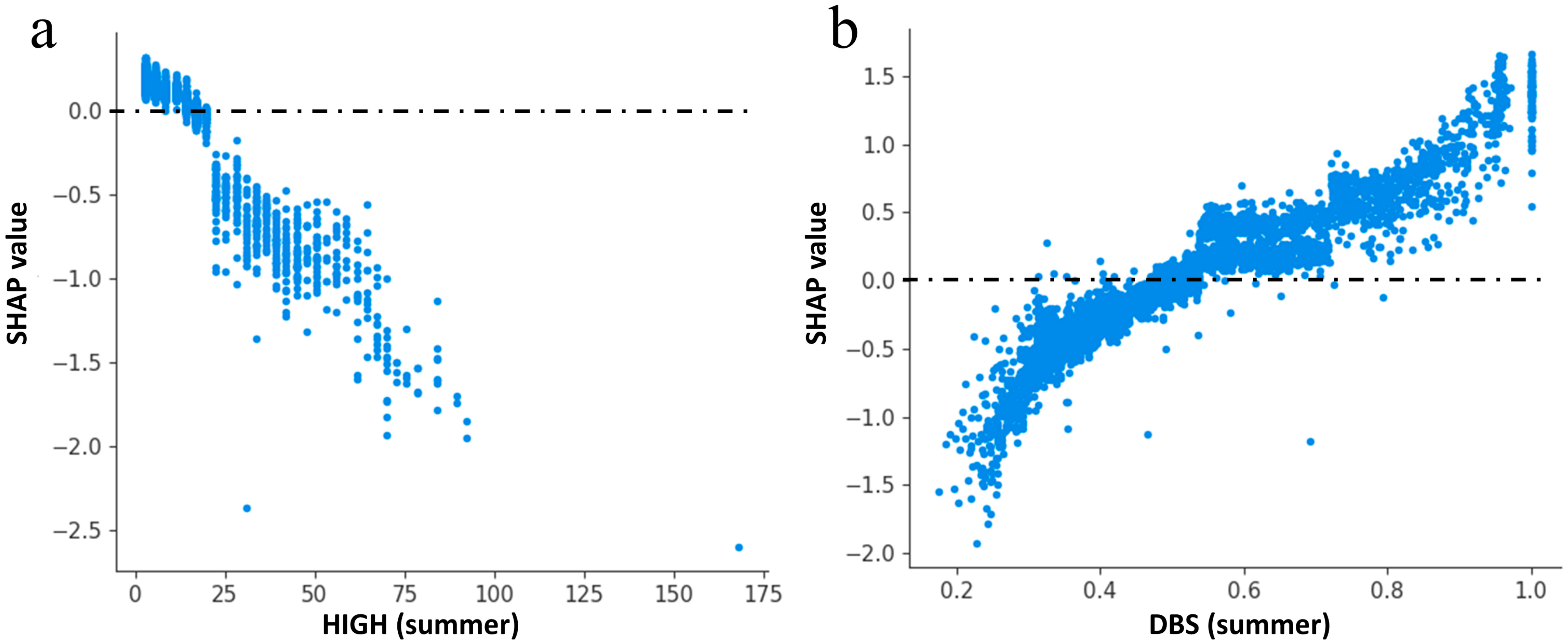
It is noteworthy to mention that the majority of prior research has simply determined that the correlation between SVF and UHII is either affirmative [64] or adverse [21]. The findings obtained from this experiment, as illustrated in Figure 6, indicate that the correlation between the two variables does not exhibit a monotonic pattern. An ascending trend is observed when the SVF value falls below 0.85, whereas a descending trend is noted when the SVF value is less than 0.85. UHII experiences a weakening trend when the SVF value is either excessively large or small. The aforementioned phenomenon can be elucidated by the notion that the impact of SVF on the temperature response is determined by the proportionate influence of the two facets it impacts. On one hand, a higher SVF value corresponds to increased openness, resulting in improved airflow and wind speed that can impact temperature. On the other hand, a higher SVF value results in greater ground exposure to solar radiation, which is a significant factor in temperature variation [65]. Based on the information gathered from the HIGH indicator, it can be inferred that the impact of high-rise buildings on mitigating the UHII is more significant in comparison to low-rise buildings. The data presented in Figure 7 indicate that the mitigation of UHII becomes significant when the height of the building surpasses 25 m. The primary factor contributing to the attenuation of UHII by taller buildings is their ability to generate greater shadowing. The impact of the height of buildings on the UHI effect may vary based on distinct urban spatial configurations and underlying climatic conditions [21,66]. Empirical findings from Shanghai, China indicate that vertical structures exceeding 30 m in height exhibit a moderating influence on the UHI effect [43]. The DBS indicator exhibits a comparable pattern to that of the FAR indicator, albeit with a greater susceptibility to the influence of UHII, as evidenced by the data presented in Figure 7b. Different shapes of buildings primarily affect the UHI effect through their impact on ventilation [67]. A homogeneous cluster of buildings of a single type may have better ventilation effects, thus mitigating the UHI [68].

The experimental findings can be verified by the energy balance equation, wherein the latent heat flux $Q_E$, which is diminished by evapotranspiration, is substituted by the sensible heat flux $Q_H$, which retains heat on the urban surface, due to the conversion of vegetation into buildings. In addition, it should be noted that the height and density of buildings have the potential to impact the magnitude and rate of the heat storage flux $\mathsf{\Delta }{Q}_S$, and thus the intensity and duration of the UHI effect [60]. Taller structures possess a greater capacity for heat storage and release, thereby exhibiting a more pronounced ability to alleviate the UHI effect. The impact of buildings on UHII can vary depending on the spatial scale [67]. Although buildings may have a cooling effect on a small scale, the proliferation of buildings in urban areas can contribute to an overall increase in UHII at larger scales. To summarize, there are varying thresholds for FAR, HIGH, SVF, and DBS in urban planning and construction, which can be utilized by managers to enhance the thermal comfort and livability of urban areas.

4.1.2. The Influence of Vegetation and Water Bodies in 2D/3D Space

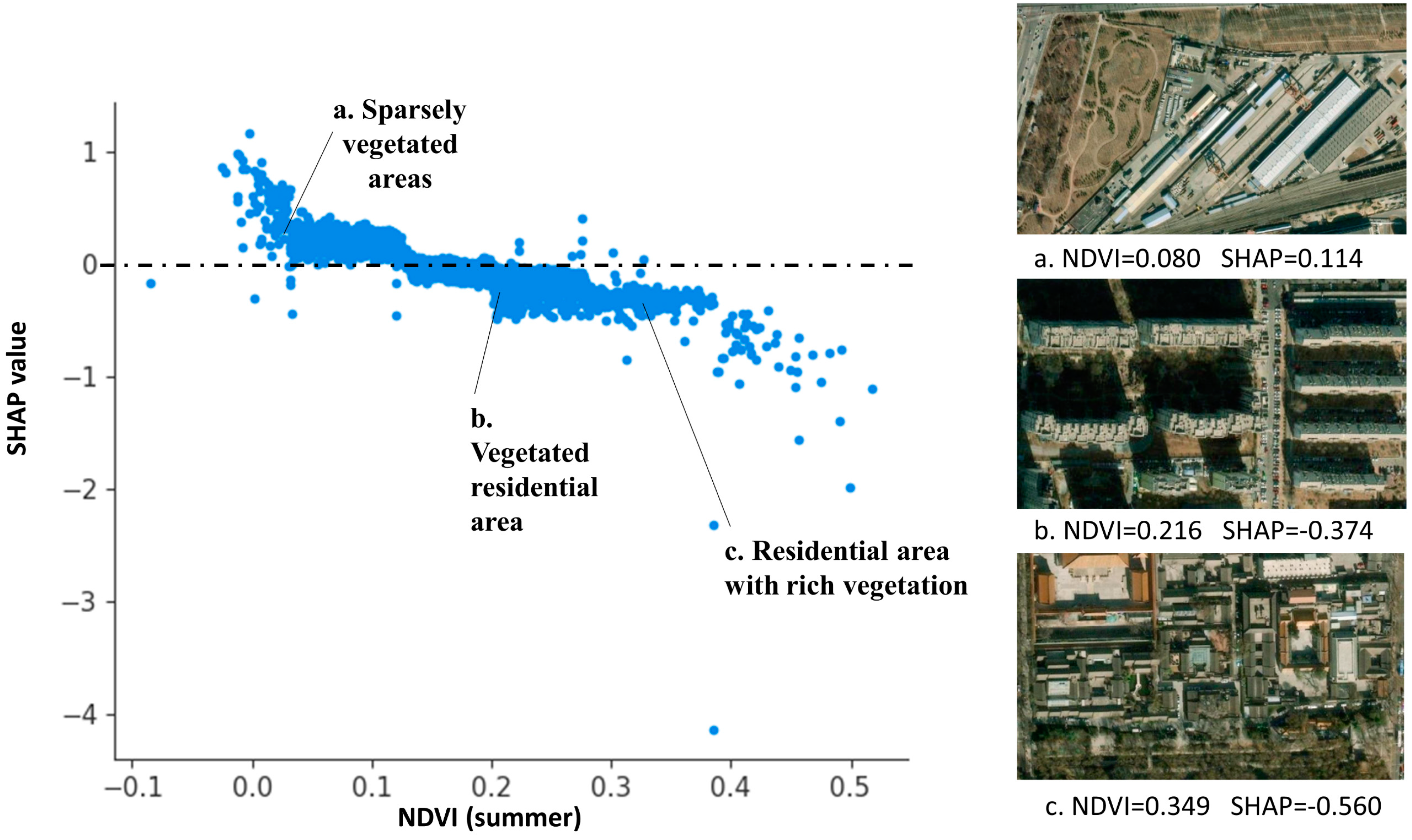
Vegetation and bodies of water are known to have a notable cooling effect on the UHI effect. A positive NDVI value is indicative of vegetation coverage within a given area. Therefore, our discussion will be limited to the portion of the area where the NDVI value is positive. It is noteworthy that SHAP values exhibit positivity in instances where NDVI is low, and conversely, they demonstrate negativity when NDVI attains higher values. Prior research endeavors exploring the association between vegetation and UHI have produced exclusively positive or negative correlations. This has been documented in various studies [69,70]. The diagram depicted in Figure 8a illustrates that regions exhibiting low NDVI values are characterized by being unpopulated, underdeveloped, and having limited vegetation. Furthermore, it is observed that such areas have a positive impact on the UHI effect. The graphical representation in Figure 8b,c reveals that regions with elevated values primarily comprise tree and grass plantations along the thoroughfares. Residential areas exhibit a verdant hue, albeit predominantly constituted of diminutive shrubs that possess the limited potential for mitigating heat islands. The variance in the size of trees can significantly influence the UHI effect, owing to the fact that larger trees have the potential to offer greater evapotranspiration and shading effects [71]. A reduced NDVI indicates that the distribution and size of vegetation are comparatively lower. This results in a limited cooling impact on the air temperature, which can be easily overshadowed by the presence of numerous heat sources in the surrounding environment [72,73]. The data presented in Figure 8 indicate that vegetation has a notable impact on mitigating the UHI effect. This effect is observed to be more pronounced when the NDVI value exceeds 0.1 and increases further. Consequently, this effect can lead to the emergence of extensive regions with lower temperatures on the map. To clarify, the evaluation of the cooling impact of vegetation can be conducted through spatial aggregation [74].

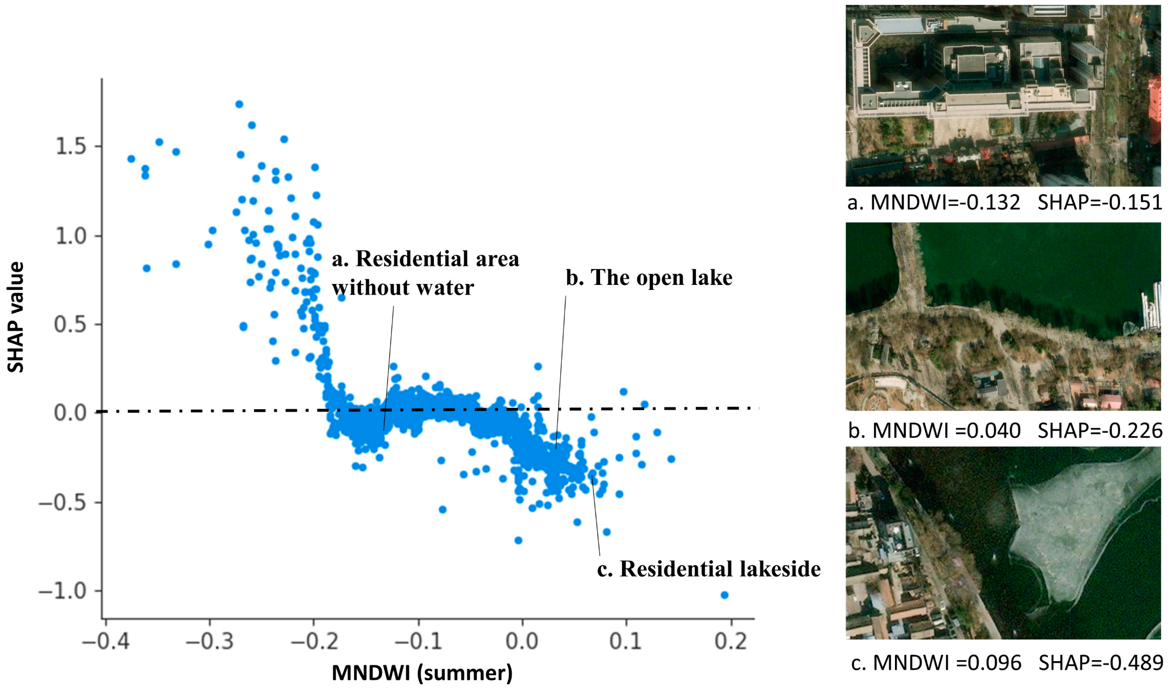
The MNDWI index, akin to the NDVI, exhibits positivity solely in the region encompassing water bodies, thereby restricting our discourse to the positive segment of the MNDWI. As depicted in Figure 9a, it is evident that in instances where the MNDWI index assumes a negative value, the region under consideration is devoid of any water bodies. As per the observations made in Figure 9b,c, an increase in the MNDWI value beyond 0 is found to be associated with a gradual enhancement of the cooling effect of the water body. This, in turn, leads to a reduction in the intensity of the UHI phenomenon. The findings of the trend analysis indicate that the impact of water bodies on mitigating the UHI effect is more immediate compared to vegetation. Specifically, the presence of water bodies in a given area tends to result in a reduction in UHI due to the higher extent and consistency of water bodies per unit of land area. However, it should be noted that the extent of water bodies’ coverage is comparatively restricted in comparison to that of vegetation, and consequently, its advantages are only accessible to a restricted population. On the contrary, the coverage of vegetation is more extensive, and can effectively alleviate the UHI effect, thereby conferring benefits to a greater populace. Hence, in densely populated urban areas where there is a scarcity of vegetation cover that is also fragmented, the most efficacious approach to mitigate the UHI effect would be to plant rapidly growing tall trees [75]. Tree species exhibit varying capacities for depression, shading, and evapotranspiration, resulting in distinct cooling effects. The promotion of tree diversity may serve as a potential strategy for mitigating UHI effects [76]. Nonetheless, the evaluation of these indices falls outside the purview of this investigation, as they cannot be quantified using three-dimensional morphometric metrics.

4.2. Implications for Urban Planning and Management

The implementation of green roofs and water features have been extensively advocated as a crucial component of intelligent urban development approaches aimed at mitigating the UHI effect [77,78]. This manuscript suggests a set of urban landscape strategies derived from experimental findings to assist urban planners in more efficiently addressing UHI. Initially, erecting high-rise structures amidst verdant landscapes and aquatic environments is a proficient tactic for alleviating the UHI effect [79]. The determination of the height threshold for tall buildings ought to be contingent upon the factual circumstances of a particular locality. In the city of Beijing, structures that exceed a height of 25 m, equivalent to eight storys, may be classified as tall buildings. The vertical expansion of buildings has the potential to alleviate the strain on finite land resources and offer additional opportunities for the creation of green spaces. Furthermore, as demonstrated in the research outlined in Section 4.1.2, it has been found that trees possess a greater capacity to alleviate the UHI effect in areas with restricted green space, as compared to grass. The study suggests that it is advisable to exercise significant control over the construction of dense, low-rise clusters of buildings, as they have been found to exert the most potent influence on the exacerbation of the UHI effect. It is recommended that urban planners promote the development of large, multistory complexes as a means of addressing the UHI effect, while also maintaining site productivity.

5. Conclusions

This paper offers a framework for measuring urban morphology, aiming to comprehensively and objectively evaluate the 2D/3D spatial patterns of cities. Using this framework, a regression analysis based on the XGBoost algorithm was performed, and the complex relationship between urban morphology and UHI was explored in the area within the Fifth Ring Road of Beijing on a 500 m × 500 m grid. In addition, a new interpretation method called SHAP was applied to compare and analyze the correlation between various spatial form indicators and seasonal UHI. The following conclusions were drawn: the daytime UHI effect within the fifth ring road is severe, with over 90% of the area experiencing varying degrees of UHI, particularly in summer and autumn, while the severity is relatively light in spring and winter; the impact of spatial form indicators on UHI varies by season, with FAR being the most correlated indicator with summer UHI and HIGH with autumn UHI, and some indicators have a more significant impact in specific seasons, such as MNDWI having a stronger impact on UHI in winter; the composition and structure of buildings are closely related to UHI, and a dispersed distribution is beneficial in mitigating UHI. The cooling effect of vegetation on UHI remains valid in the three-dimensional measurement system, with a larger proportion of vegetation in space showing a greater cooling effect on UHI.

Based on the above research findings, we suggest that when it comes to optimizing urban spatial forms to mitigate the UHI effect in urban design and spatial planning, attention should be paid to seasonal, spatial, and indicator-specific considerations. From a seasonal perspective, the study shows that in the Beijing Fifth Ring area, summer and autumn are the periods when the daytime UHI effect is particularly severe, while it is relatively mild in spring and winter. Therefore, it is necessary to formulate strategies mainly to alleviate the UHI effect according to different seasons. In addition, we also need to consider that different indicators have different contributions to the urban heat environment in different seasons. Therefore, when choosing the indicators to be adjusted for morphological optimization, we should select the indicators with a larger contribution in combination with the impact of the seasons to improve the effectiveness of the adjustment strategy.

It should be noted that this study only considered surface temperature data during summer daytime, lacking nighttime data. Therefore, the conclusions drawn are only applicable to daytime urban heat environment optimization. We also need further in-depth research to explore the impact of the nighttime UHI effect on urban heat environment optimization and to find corresponding solutions. Due to the limitations of the study scope and data availability, there are several unexplored directions in urban morphology research that can enhance our understanding of the UHI effect. These factors include different vegetation types, biomass, as well as factors such as precipitation, wind direction, and wind speed that influence the daily UHI.

References

1. Mohajerani, A.; Bakaric, J.; Jeffrey-Bailey, T. The urban heat island effect, its causes, and mitigation, with reference to the thermal properties of asphalt concrete. J. Environ. Manag. 2017, 197, 522–538. [Google Scholar] [CrossRef]
2. Yu, Z.; Zhang, J.; Yang, G. How to build a heat network to alleviate surface heat island effect? Sustain. Cities Soc. 2021, 74, 103135. [Google Scholar] [CrossRef]
3. Oke, T.R. The energetic basis of the urban heat island. Q. J. R. Meteorol. Soc. 1982, 108, 1–24. [Google Scholar] [CrossRef]
4. Grimm, N.B.; Faeth, S.H.; Golubiewski, N.E.; Redman, C.L.; Wu, J.; Bai, X.; Briggs, J.M. Global change and the ecology of cities. Science 2008, 319, 756–760. [Google Scholar] [CrossRef] [Green Version]
5. Lo, C.P.; Quattrochi, D.A.; Luvall, J.C. Application of high-resolution thermal infrared remote sensing and GIS to assess the urban heat island effect. Int. J. Remote Sens. 1997, 18, 287–304. [Google Scholar] [CrossRef] [Green Version]
6. Adeyemi, A.; Ramoelo, A.; Cho, M.A.; Strydom, J. Spatio-temporal analysis of built-up impervious surface area and interplay with land surface temperature in Pretoria, South Africa. Geocarto Int. 2022, 37, 7618–7638. [Google Scholar] [CrossRef]
7. Allegrini, J.; Carmeliet, J. Coupled CFD and building energy simulations for studying the impacts of building height topology and buoyancy on local urban microclimates. Urban Clim. 2017, 21, 278–305. [Google Scholar] [CrossRef]
8. Zheng, B.H.; Bedra, K.B.; Zheng, J.; Wang, G.G. Combination of Tree Configuration with Street Configuration for Thermal Comfort Optimization under Extreme Summer Conditions in the Urban Center of Shantou City, China. Sustainability 2018, 10, 4192. [Google Scholar] [CrossRef] [Green Version]
9. Tran, D.X.; Pla, F.; Latorre-Carmona, P.; Myint, S.W.; Caetano, M.; Kieu, H.V. Characterizing the relationship between land use land cover change and land surface temperature. ISPRS J. Photogramm. Remote Sens. 2017, 124, 119–132. [Google Scholar] [CrossRef] [Green Version]
10. Huang, X.; Wang, Y. Investigating the effects of 3D urban morphology on the surface urban heat island effect in urban functional zones by using high-resolution remote sensing data: A case study of Wuhan, Central China. ISPRS J. Photogramm. Remote Sens. 2019, 152, 119–131. [Google Scholar] [CrossRef]
11. Guo, G.; Wu, Z.; Xiao, R.; Chen, Y.; Liu, X.; Zhang, X. Impacts of urban biophysical composition on land surface temperature in urban heat island clusters. Landsc. Urban Plan. 2015, 135, 1–10. [Google Scholar] [CrossRef]
12. Liang, Z.; Wu, S.Y.; Wang, Y.Y.; Wei, F.L.; Huang, J.; Shen, J.S.; Li, S.C. The relationship between urban form and heat island intensity along the urban development gradients. Sci. Total Environ. 2020, 708, 135011. [Google Scholar] [CrossRef] [PubMed]
13. Oke, T.R. City size and the urban heat island. Atmos. Environ. 1973, 7, 769–779. [Google Scholar] [CrossRef]
14. Monteiro, M.V.; Doick, K.J.; Handley, P.; Peace, A. The impact of greenspace size on the extent of local nocturnal air temperature cooling in London. Urban For. Urban Green. 2016, 16, 160–169. [Google Scholar] [CrossRef]
15. Scarano, M.; Mancini, F. Assessing the relationship between sky view factor and land surface temperature to the spatial resolution. Int. J. Remote Sens. 2017, 38, 6910–6929. [Google Scholar] [CrossRef]
16. Huang, X.; Chen, H.; Gong, J. Angular difference feature extraction for urban scene classification using ZY-3 multi-angle high-resolution satellite imagery. ISPRS J. Photogramm. Remote Sens. 2018, 135, 127–141. [Google Scholar] [CrossRef]
17. Guan, Q.; Yao, Y.; Ma, T.; Hong, Y.; Bie, Y.; Lyu, J. Under the Dome: A 3D Urban Texture Model and Its Relationship with Urban Land Surface Temperature. Ann. Am. Assoc. Geogr. 2021, 112, 1369–1389. [Google Scholar] [CrossRef]
18. Zhou, Y.; Zhao, H.; Mao, S.; Zhang, G.; Jin, Y.; Luo, Y.; Huo, W.; Pan, Z.; An, P.; Lun, F. Exploring surface urban heat island (SUHI) intensity and its implications based on urban 3D neighborhood metrics: An investigation of 57 Chinese cities. Sci. Total Environ. 2022, 847, 157662. [Google Scholar] [CrossRef]
19. Li, J.; Song, C.; Cao, L.; Zhu, F.; Meng, X.; Wu, J. Impacts of landscape structure on surface urban heat islands: A case study of Shanghai, China. Remote Sens. Environ. 2011, 115, 3249–3263. [Google Scholar] [CrossRef]
20. Wu, C.-D.; Lung, S.-C.C. Application of 3-D urbanization index to assess impact of urbanization on air temperature. Sci. Rep. 2016, 6, 24351. [Google Scholar] [CrossRef]
21. Berger, C.; Rosentreter, J.; Voltersen, M.; Baumgart, C.; Schmullius, C.; Hese, S. Spatio-temporal analysis of the relationship between 2D/3D urban site characteristics and land surface temperature. Remote Sens. Environ. 2017, 193, 225–243. [Google Scholar] [CrossRef]
22. Uyanık, G.K.; Güler, N. A study on multiple linear regression analysis. Procedia-Soc. Behav. Sci. 2013, 106, 234–240. [Google Scholar] [CrossRef] [Green Version]
23. Ostertagová, E. Modelling using polynomial regression. Procedia Eng. 2012, 48, 500–506. [Google Scholar] [CrossRef] [Green Version]
24. Mahesh, B. Machine learning algorithms-a review. Int. J. Sci. Res. IJSR 2020, 9, 381–386. [Google Scholar]
25. Molnar, C. Interpretable Machine Learning; Lulu Press: Morrisville, NC, USA, 2020. [Google Scholar]
26. Guidotti, R.; Monreale, A.; Ruggieri, S.; Turini, F.; Giannotti, F.; Pedreschi, D. A survey of methods for explaining black box models. ACM Comput. Surv. CSUR 2018, 51, 1–42. [Google Scholar] [CrossRef] [Green Version]
27. Gao, Y.; Zhao, J.; Han, L. Quantifying the nonlinear relationship between block morphology and the surrounding thermal environment using random forest method. Sustain. Cities Soc. 2023, 91, 104443. [Google Scholar] [CrossRef]
28. Kim, M.; Kim, G. Modeling and Predicting Urban Expansion in South Korea Using Explainable Artificial Intelligence (XAI) Model. Appl. Sci. 2022, 12, 9169. [Google Scholar] [CrossRef]
29. Du, Y.; McNestry, C.; Wei, L.; Antoniadi, A.M.; McAuliffe, F.M.; Mooney, C. Machine learning-based clinical decision support systems: A systematic review. Appl. Sci. 2021, 11, 5088. [Google Scholar] [CrossRef]
30. Iban, M.C. An explainable model for the mass appraisal of residences: The application of tree-based Machine Learning algorithms and interpretation of value determinants. Habitat Int. 2022, 128, 102660. [Google Scholar] [CrossRef]
31. Yang, Q.; Huang, X.; Tang, Q. The footprint of urban heat island effect in 302 Chinese cities: Temporal trends and associated factors. Sci. Total Environ. 2019, 655, 652–662. [Google Scholar] [CrossRef]
32. Middel, A.; Häb, K.; Brazel, A.J.; Martin, C.A.; Guhathakurta, S. Impact of urban form and design on mid-afternoon microclimate in Phoenix Local Climate Zones. Landsc. Urban Plan. 2014, 122, 16–28. [Google Scholar] [CrossRef]
33. Alobaydi, D.; Bakarman, M.A.; Obeidat, B. The Impact of Urban Form Configuration on the Urban Heat Island: The Case Study of Baghdad, Iraq. Procedia Eng. 2016, 145, 820–827. [Google Scholar] [CrossRef]
34. Bourdic, L.; Salat, S.; Nowacki, C. Assessing cities: A new system of cross-scale spatial indicators. Build. Res. Inf. 2012, 40, 592–605. [Google Scholar] [CrossRef]
35. Qin, Z.; Wenjuan, L.; Minghua, Z.; Karnieli, A.; Berliner, P. Estimating of the essential atmospheric parameters of mono-window algorithm for land surface temperature retrieval from lanDSAT TM6. Remote Sens. Land Resour. 2003, 15, 37–43. [Google Scholar]
36. Howard, L. The Climate of London: Deduced from Meteorological Observations; Cambridge University Press: Cambridge, UK, 2012; Volume 1. [Google Scholar]
37. Quan, J.; Zhan, W.; Chen, Y.; Wang, M.; Wang, J. Time series decomposition of remotely sensed land surface temperature and investigation of trends and seasonal variations in surface urban heat islands. J. Geophys. Res. Atmos. 2016, 121, 2638–2657. [Google Scholar] [CrossRef]
38. Jiang, J.; Zhou, Y.; Guo, X.; Qu, T. Calculation and Expression of the Urban Heat Island Indices Based on GeoSOT Grid. Sustainability 2022, 14, 2588. [Google Scholar] [CrossRef]
39. Li, K.; Chen, Y.; Wang, M.; Gong, A. Spatial-temporal variations of surface urban heat island intensity induced by different definitions of rural extents in China. Sci. Total Environ. 2019, 669, 229–247. [Google Scholar] [CrossRef] [PubMed]
40. Zhang, X.; Liu, L.; Wu, C.; Chen, X.; Gao, Y.; Xie, S.; Zhang, B. Development of a global 30 m impervious surface map using multisource and multitemporal remote sensing datasets with the Google Earth Engine platform. Earth Syst. Sci. Data 2020, 12, 1625–1648. [Google Scholar] [CrossRef]
41. Peng, S.; Piao, S.; Ciais, P.; Friedlingstein, P.; Ottle, C.; Bréon, F.-M.; Nan, H.; Zhou, L.; Myneni, R.B. Surface urban heat island across 419 global big cities. Environ. Sci. Technol. 2012, 46, 696–703. [Google Scholar] [CrossRef] [PubMed]
42. Chen, T.; Guestrin, C. Xgboost: A Scalable Tree Boosting System. In Proceedings of the 22nd ACM SIGKDD International Conference on Knowledge Discovery and Data Mining, San Francisco, CA, USA, 13–17 August 2016; pp. 785–794. [Google Scholar]
43. Yu, S.; Chen, Z.; Yu, B.; Wang, L.; Wu, B.; Wu, J.; Zhao, F. Exploring the relationship between 2D/3D landscape pattern and land surface temperature based on explainable eXtreme Gradient Boosting tree: A case study of Shanghai, China. Sci. Total Environ. 2020, 725, 138229. [Google Scholar] [CrossRef]
44. Zhao, X.Z.; Yu, B.L.; Liu, Y.; Chen, Z.Q.; Li, Q.X.; Wang, C.X.; Wu, J.P. Estimation of Poverty Using Random Forest Regression with Multi-Source Data: A Case Study in Bangladesh. Remote Sens. 2019, 11, 375. [Google Scholar] [CrossRef] [Green Version]
45. Molnar, C.; Casalicchio, G.; Bischl, B. Interpretable machine learning—A brief history, state-of-the-art and challenges. In Proceedings of the ECML PKDD 2020 Workshops: Workshops of the European Conference on Machine Learning and Knowledge Discovery in Databases (ECML PKDD 2020): SoGood 2020, PDFL 2020, MLCS 2020, NFMCP 2020, DINA 2020, EDML 2020, XKDD 2020 and INRA 2020, Ghent, Belgium, 14–18 September 2020; Springer: Berlin/Heidelberg, Germany, 2021; pp. 417–431. [Google Scholar]
46. Dabkowski, P.; Gal, Y. Real time image saliency for black box classifiers. In Proceedings of the Annual Conference on Neural Information Processing Systems 2017, Long Beach, CA, USA, 4–9 December 2017. [Google Scholar]
47. Shapley, L.S. A Value for n-Person Games; Princeton University Press: Princeton, NJ, USA, 1953. [Google Scholar]
48. Lundberg, S.M.; Erion, G.G.; Lee, S.-I. Consistent Individualized Feature Attribution for Tree Ensembles. arXiv 2018, arXiv:1802.03888. [Google Scholar]
49. Beijing Overview. Available online: http://www.beijing.gov.cn/renwen/bjgk (accessed on 15 March 2023).
50. Beijing Municipal Bureau of Statistics. Available online: http://tjj.beijing.gov.cn (accessed on 15 March 2023).
51. Li, Z.; Zhao, Y.; Hu, D. Evaluating the impacts of three-dimensional building morphology on urban near-surface energy fluxes: A case study in Beijing, China. Energy Build. 2023, 279, 112690. [Google Scholar] [CrossRef]
52. Jenks, G.F. Optimal Data Classification for Choropleth Maps; Occasional Paper; Department of Geography, University of Kansas: Lawrence, KS, USA, 1977. [Google Scholar]
53. Peng, W.C.Y.; Wang, R.; Duan, J.; Gao, W.J.; Fan, Z.X. Surface and canopy urban heat islands: Does urban morphology result in the spatiotemporal differences? Urban Clim. 2022, 42, 101136. [Google Scholar] [CrossRef]
54. Cai, Z.; Han, G.F.; Chen, M.C. Do water bodies play an important role in the relationship between urban form and land surface temperature? Sustain. Cities Soc. 2018, 39, 487–498. [Google Scholar] [CrossRef]
55. Murakawa, S.; Sekine, T.; Narita, K.-I.; Nishina, D. Study of the effects of a river on the thermal environment in an urban area. Energy Build. 1991, 16, 993–1001. [Google Scholar] [CrossRef]
56. Xi, C.; Ren, C.; Wang, J.; Feng, Z.; Cao, S.-J. Impacts of urban-scale building height diversity on urban climates: A case study of Nanjing, China. Energy Build. 2021, 251, 111350. [Google Scholar] [CrossRef]
57. Chen, J.; Du, P.; Jin, S.; Ding, H.; Chen, C.; Xu, Y.; Feng, L.; Guo, G.; Zheng, H.; Huang, M. Unravelling the multilevel and multi-dimensional impacts of building and tree on surface urban heat islands. Energy Build. 2022, 259, 111843. [Google Scholar] [CrossRef]
58. Wang, Q.; Fan, Y.; Hang, J.; Li, Y. Interacting urban heat island circulations as affected by weak background wind. Build. Environ. 2019, 160, 106224. [Google Scholar] [CrossRef]
59. Chun, B.; Guldmann, J.M. Impact of greening on the urban heat island: Seasonal variations and mitigation strategies. Comput. Environ. Urban Syst. 2018, 71, 165–176. [Google Scholar] [CrossRef]
60. Oke, T.R.; Mills, G.; Christen, A.; Voogt, J.A. Urban Climates; Cambridge University Press: Cambridge, UK, 2017. [Google Scholar]
61. Oke, T.R. The urban energy balance. Prog. Phys. Geogr. 1988, 12, 471–508. [Google Scholar] [CrossRef]
62. Guo, G.; Zhou, X.; Wu, Z.; Xiao, R.; Chen, Y. Characterizing the impact of urban morphology heterogeneity on land surface temperature in Guangzhou, China. Environ. Model. Softw. 2016, 84, 427–439. [Google Scholar] [CrossRef]
63. Lan, Y.; Zhan, Q. How do urban buildings impact summer air temperature? The effects of building configurations in space and time. Build. Environ. 2017, 125, 88–98. [Google Scholar] [CrossRef]
64. Yang, F.; Lau, S.S.Y.; Qian, F. Summertime heat island intensities in three high-rise housing quarters in inner-city Shanghai China: Building layout, density and greenery. Build. Environ. 2010, 45, 115–134. [Google Scholar] [CrossRef]
65. Yang, X.; Li, Y. The impact of building density and building height heterogeneity on average urban albedo and street surface temperature. Build. Environ. 2015, 90, 146–156. [Google Scholar] [CrossRef]
66. Zhao, L.; Lee, X.; Smith, R.B.; Oleson, K. Strong contributions of local background climate to urban heat islands. Nature 2014, 511, 216–219. [Google Scholar] [CrossRef]
67. Gao, Y.; Yao, R.; Li, B.; Turkbeyler, E.; Luo, Q.; Short, A. Field studies on the effect of built forms on urban wind environments. Renew. Energy 2012, 46, 148–154. [Google Scholar] [CrossRef]
68. Jiang, Y.; Wu, C.; Teng, M. Impact of residential building layouts on microclimate in a high temperature and high humidity region. Sustainability 2020, 12, 1046. [Google Scholar] [CrossRef] [Green Version]
69. Cheng, X.; Wei, B.; Chen, G.; Li, J.; Song, C. Influence of park size and its surrounding urban landscape patterns on the park cooling effect. J. Urban Plan. Dev. 2015, 141, A4014002. [Google Scholar] [CrossRef]
70. Al-Saadi, L.M.; Jaber, S.H.; Al-Jiboori, M.H. Variation of urban vegetation cover and its impact on minimum and maximum heat islands. Urban Clim. 2020, 34, 100707. [Google Scholar] [CrossRef]
71. Park, Y.; Guldmann, J.-M.; Liu, D. Impacts of tree and building shades on the urban heat island: Combining remote sensing, 3D digital city and spatial regression approaches. Comput. Environ. Urban Syst. 2021, 88, 101655. [Google Scholar] [CrossRef]
72. Zhang, Y.; Zhan, Y.; Yu, T.; Ren, X. Urban green effects on land surface temperature caused by surface characteristics: A case study of summer Beijing metropolitan region. Infrared Phys. Technol. 2017, 86, 35–43. [Google Scholar] [CrossRef]
73. Das, M.; Das, A.; Momin, S. Quantifying the cooling effect of urban green space: A case from urban parks in a tropical mega metropolitan area (India). Sustain. Cities Soc. 2022, 87, 104062. [Google Scholar] [CrossRef]
74. Armson, D.; Stringer, P.; Ennos, A. The effect of tree shade and grass on surface and globe temperatures in an urban area. Urban For. Urban Green. 2012, 11, 245–255. [Google Scholar] [CrossRef]
75. Tan, J.K.; Belcher, R.N.; Tan, H.T.; Menz, S.; Schroepfer, T. The urban heat island mitigation potential of vegetation depends on local surface type and shade. Urban For. Urban Green. 2021, 62, 127128. [Google Scholar] [CrossRef]
76. Wang, X.; Dallimer, M.; Scott, C.E.; Shi, W.; Gao, J. Tree species richness and diversity predicts the magnitude of urban heat island mitigation effects of greenspaces. Sci. Total Environ. 2021, 770, 145211. [Google Scholar] [CrossRef]
77. Oberndorfer, E.; Lundholm, J.; Bass, B.; Coffman, R.R.; Doshi, H.; Dunnett, N.; Gaffin, S.; Köhler, M.; Liu, K.K.; Rowe, B. Green roofs as urban ecosystems: Ecological structures, functions, and services. BioScience 2007, 57, 823–833. [Google Scholar] [CrossRef]
78. Gober, P.; Brazel, A.; Quay, R.; Myint, S.; Grossman-Clarke, S.; Miller, A.; Rossi, S. Using watered landscapes to manipulate urban heat island effects: How much water will it take to cool Phoenix? J. Am. Plan. Assoc. 2009, 76, 109–121. [Google Scholar] [CrossRef]
79. Deilami, K.; Kamruzzaman, M.; Liu, Y. Urban heat island effect: A systematic review of spatio-temporal factors, data, methods, and mitigation measures. Int. J. Appl. Earth Obs. Geoinf. 2018, 67, 30–42. [Google Scholar] [CrossRef]
Figure 1. The background temperature field region.
Sustainability 15 10787 g001
Figure 2. Location map of Beijing’s Fifth Ring Road area (the left map shows geographical location information and the right map shows the spatial distribution of buildings within the Fifth Ring Road).
Sustainability 15 10787 g002
Figure 3. UHII distribution in all seasons with two samples’ aerial photos.
Sustainability 15 10787 g003
Figure 4. Summary of SHAP feature maps for XGBoost models based on four seasons: (a) spring; (b) summer; (c) autumn; (d) winter.
Sustainability 15 10787 g004
Figure 5. SHAP dependency plots for FAR with three samples’ aerial photos.
Sustainability 15 10787 g005
Figure 6. SHAP dependency plots for SVF with three samples’ aerial photos.
Sustainability 15 10787 g006
Figure 7. SHAP dependency plots for HIGH (a) and DBS (b).
Sustainability 15 10787 g007
Figure 8. SHAP dependency plots for NDVI with three samples’ aerial photos.
Sustainability 15 10787 g008
Figure 9. SHAP dependency plots for MNDWI with three samples’ aerial photos.
Sustainability 15 10787 g009