Article

Residual Neural Networks for Origin–Destination Trip Matrix Estimation from Traffic Sensor Information

1
Department of Civil and Environmental Engineering, College of Engineering, Majmaah University, Majmaah 11952, Saudi Arabia
2
Civil Engineering Department, Faculty of Engineering, Assiut University, Assiut 71516, Egypt
3
Civil Engineering Department, Faculty of Engineering, Sphinx University, New Assiut 71515, Egypt
4
Department of Computer Science, College of Computer and Information Sciences, Majmaah University, Majmaah 11952, Saudi Arabia
5
Department of Architecture and Planning, College of Engineering, King Khalid University, Abha 61421, Saudi Arabia
*
Author to whom correspondence should be addressed.
Sustainability 2023, 15(13), 9881; https://doi.org/10.3390/su15139881
Submission received: 13 April 2023 / Revised: 2 June 2023 / Accepted: 15 June 2023 / Published: 21 June 2023

Abstract

:
Traffic management and control applications require comprehensive knowledge of traffic flow data. Typically, such information is gathered using traffic sensors, which have two basic challenges: First, it is impractical or impossible to install sensors on every arc in a network. Second, sensors do not provide direct information on origin-to-destination (O–D) demand flows. Consequently, it is essential to identify the optimal locations for deploying traffic sensors and then enhance the knowledge gained from this link flow sample to forecast the network’s traffic flow. This article presents residual neural networks—a very deep set of neural networks—to the problem for the first time. The suggested architecture reliably predicts the whole network’s O–D flows utilizing link flows, hence inverting the standard traffic assignment problem. It deduces a relevant correlation between traffic flow statistics and network topology from traffic flow characteristics. To train the proposed deep learning architecture, random synthetic flow data was generated from the historical demand data of the network. A large-scale network was used to test and confirm the model’s performance. Then, the Sioux Falls network was used to compare the results with the literature. The robustness of applying the proposed framework to this particular combined traffic flow problem was determined by maintaining superior prediction accuracy over the literature with a moderate number of traffic sensors.

1. Introduction

Transportation planning and operations in megacities require information on traffic flow. Incomplete or inadequate flow data impede the implementation of the majority of intelligent transportation systems. The origin–destination (O–D) demand matrix is a crucial datum type. Traffic analysts and operators aim to obtain accurate O–D data to make sound strategic, tactical, and operational choices. In both static and dynamic approaches, an O–D matrix may be readily translated into various flow data types (i.e., path and link flow). This transformation is the result of addressing the well-known traffic assignment problem [1,2]. The literature is replete with models for traffic assignment that use different efficient solution strategies [3,4].
Traffic counts on transportation network streets/links provide the most reliable traffic information. Unfortunately, placing sensors on all network links is unaffordable due to the expense of sensor installation relative to the number of sensors required to cover all links in a real-world network of moderate scale. Even if all network links are equipped with sensors, none of the traffic assignment models offer an inverse formula for estimating the O–D matrix causing the observed flows [2].
O–D estimate techniques are always based on prior data. Historical O–D matrices are the most prevalent form used to direct the search process. Consequently, a substantial portion of the estimating method’s precision is contingent on the dependability of the O–D data, which often originates from historical records. The correctness of the estimated O–D matrix is determined by its capacity to create the flows required in its estimation with the smallest variation possible from the historical O–D matrix [5].
In contrast, the distribution of network traffic sensors is not a simple matter. The combinatorial complexity of the problem makes real-world transportation networks challenging. From a multidisciplinary standpoint, the problem is simple to formulate yet challenging to solve. The TSLP efficiently finds network links or nodes equipped with a certain traffic sensor in order to collect specified flow statistics [6,7]. Multiple strategies for sensor placement on a network might facilitate data collecting, which could be beneficial for traffic management and control. Depending on the importance of the information, several TSLP solution options may be utilized to handle this issue. To obtain a comprehensive picture of the flows of interest in this circumstance, it is essential to evaluate the placement of the sensors in addition to the amount and quality of the readings [8]. The problem is further exacerbated by the addition of other factors, such as installation objectives, sensor type, budget limitations, sensor error/failure rates, and optimality criteria [9].
Numerous sensing technologies are now in use, including piezoelectric-based weight-in-motion sensors, inductive loops, laser sensors, triple technology (passive, radar, and ultrasonic sensors), and image recognition (video systems). Theoretical study identifies two core systems: passive and active sensors. The passive sensor system is solely concerned with link volumes as simple vehicle counts. On the other hand, active sensor systems can offer extra information on vehicle type, license ID, and time stamp of vehicle observation. In fact, these extra pieces of information enable the designer to employ more advanced analytical models to gain a deeper understanding of the data or a more clear understanding of traffic circumstances. However, the high expense of establishing these active systems is associated with this enhanced knowledge [10]. Passive, active, or heterogeneous (i.e., a combination of active and passive sensors) should be stated first as the type of sensing mode employed in TSLP research [11]. This study is concerned with the most available and cheapest tool in practice (i.e., passive counting system).
The research question posed is bidimensional. The first dimension searches the method to derive a correct O-D matrix from traffic counts. The second dimension tries to find the ideal number and placement of sensors to perform the first job efficiently. In the literature, their respective names refer to the O–D estimation problem (ODEP) and the traffic sensor location problem (TSLP). The two issues have several intricacies [12,13], making their integration into a single-solution technique intriguing. This study makes a novel addition to the ODEP by using innovative machine learning to solve the problem, for the first time, to the best of the authors’ knowledge, with a complete framework to solve the ODEP and the TSLP together. Following is the continuation of this article. Section 2 examines past ODEP–TSLP solution approaches in an effort to emphasize the gap that this work fills. In Section 3, the mathematical formulation of the problem is presented. The methodology for the solution is described in Section 4. The technique outcomes are discussed in Section 5. Section 6 concludes the work conducted in the current research.

2. Background

This part examines studies exploring ODE–TSLP as a bilevel or two-stage issue. The ODEP and TSLP are solved concurrently or sequentially to minimize the difference between the actual and expected traffic flows while optimizing the sensor locations and numbers. In addition, the evaluation is expanded to include ML applications in traffic flow forecasting to demonstrate that adapting the chosen ML approach to the suggested topic is a novel contribution. The comprehensive assessment of [8] found that, among all TSLP themes, ODE garnered the most attention. Additionally, it was the first effort to address the TSLP [14]. The challenge may be stated succinctly as how to disperse the least amount of traffic sensors to produce the most precise O–D matrix. The acquired precision depends on the sensor’s estimating approach and spatial structure. However, it has been demonstrated that sensor dispersion has the upper hand in deciding absolute accuracy. The only inherent difficulty is that the TSLP solution method cannot be immediately included in O–D estimate approaches. Consequently, the TSLP’s formulation has faced further obstacles [15].

2.1. ODE Problem

ODEP is a pioneering data analysis application of in-street monitored traffic flow [16]. In the last three decades, there have been several attempts to quantify O–D data information. Using statistical techniques such as entropy maximization [17], least squares [18], maximum likelihood [19], and Bayesian networks [20], intense research has been provided to determine the most accurate O–D matrix. The three fundamental components of traffic flow data are O–D demand, link flow, and route flow. These components are interconnected by a single hierarchy of traffic flow propagation concepts. Existing O–D trip tables are partitioned into many pathways based on user behavior, assuming network equilibrium. The link flows are the product of the path flow vector and the link–path incidence matrix. In addition, both link and path choice probabilities may be utilized to show the presumed network equilibrium [21]. Passive sensors placed directly on the targeted streets can monitor the lowest levels of the hierarchy (link flows). Path flows must be detected using path ID sensors or calculated using other active sensor systems [22]. All sensor types often presume that O–D fluxes are directly unobservable [1,5]. Links may be equipped with any form of sensor, whereas network nodes need sensors that can monitor flow turning ratios and count the number of cars at a junction. This might be considered an essential hypothesis that provides a solid basis for the mathematical treatment of the problem [6].
Lam and Lo [17] developed the idea of vital links to improve the predicted O–D matrix’s quality. The best factor for picking these links was traffic volume. Yang et al. [14] developed the maximum potential relative error (MPRE) indicator, which assesses the greatest possible difference between the anticipated and real O–D matrices. This indicator is superior since its assessment is predicated on the fact that the real O–D matrix is unknown. Specific criteria must exist beforehand for the position of the counts to constrain the MPRE value. Yang and Zhou [23] outlined four principles for positioning heuristic sensors to reduce the predicted MPRE. These are called coverage rules and have gained prominence in the literature. Bianco et al. [6] designed a two-stage iterative method to experiment with several link selection criteria to satisfy coverage restrictions. Ehlert et al. [24] employed several binary integer linear programming (BIP) formulations to accomplish full O–D coverage and maintain the MPRE’s boundness. The maximum total demand deviation (TD) was established by Bierlaire [25] as an error-bounding scale similar to the MPRE.
In all these models, the route choice proportions and the link flows in the road network are assumed to be the input data, while the trip flow matrix is the output. However, the resulting route choice proportions are inconsistent with the assumed when the estimated matrix is used in the assignment model (congestion effect). To overcome this dilemma, some studies have formulated ODEP as a bilevel problem. The upper-level problem deals with the ODEP given a set of observed links, whereas the lower-level problem tracks the estimated flow pattern to coincide with either user equilibrium (UE) or stochastic user equilibrium (SUE) flow assignment [26,27,28,29,30].
To obviate the complexity of the bilevel formulation, path flows are estimated as an indirect approach for the ODEP. The path flow estimator (PFE) was originally developed in [31]. It uses the variation in traffic flows to update the information in the traffic assignment stage and link congestion levels. This helps to identify the O–D matrix that simultaneously conserves the equilibrium in the network and produces the same observed flow on links. The attractiveness of PFE lies in the fact that it is a single-level mathematical program in which the interdependency between the O–D trip table and route choice proportion (i.e., congestion effect) is taken into account without using the bilevel mathematical program [32,33,34,35,36].
Based on the assumption that target observability elements are multivariate normal distribution, the ODEP was extended to incorporate Bayesian statistics to update the prior information and variance–covariance matrix of the variables using conditional probability among them [37,38]. In [20], conditional probability was drawn using a Bayesian network for a better representation of the estimation variables. Castillo et al. [21] examined Bayesian networks for the challenge of picking the connections based on the convergence of the Bayesian network while taking the inaccuracy of the estimated matrix into account.

2.2. The Traffic Sensor Location Problem

Owais et al. [1] recently included the MPRE directly into a random priority meta-heuristic to eliminate the requirement for high-quality a priori knowledge in order to generate a more accurate O–D matrix. In order to lower the MPRE, they simultaneously solved the TSLP as a min–max optimization model. The provided technique is surprisingly insensitive to the O–D estimate method. Salari et al. [13] enhanced prior work [1] by addressing the time-dependent sensor failure effect while taking sensor lifespan into account. Owais and Matouk [2] created a new mathematical solution method to the problem using a factorization approach. They employed backward substitution to provide the ODEP with a precise answer. Nonetheless, network scalability remains an issue for such precise systems. Owais and Shahin [12] explored both heuristic and precise solution strategies for the TSLP, taking into account the complete O–D pair coverage problem.
Castillo et al. [39] developed a different strategy by creating a linear system of equations to relate unobserved O–D pair flow with observed flows (e.g., link flows, node flows, and path flow). Castillo et al. [40] proposed a polynomial solution technique for the specified linear equation system. In contrast, Castillo et al. [41] created a complete matrix tool that incorporates all flow aspects and represents O–D flows as binary variables (0 or 1). Chen et al. [42] resolved the issue by deploying sensors to intercept all understudy O–D pairings using four BIP formulations. Then, the genetic algorithm (GA) used to solve the formulas was described. A route estimator approach was utilized to anticipate the dependability of the predicted O–D matrix without directly including it in the GA’s fitness function. Fei et al. [43] extended the same BIP formulations to time-expanded networks using the same BIP formulations. Using the generalized least squares for the ODEP and Kalman filtering techniques, they identified the TSLP’s crucial linkages. In order to expand the work of [43] to multi-objective problems, Fei and Mahmassani [44] created a hybrid greedy randomized adaptive search strategy. The model selects links based on O–D pair coverage and the data gathered by placing the sensor on that connection.
If the abovementioned ODEP–TSLP is classified as a traffic flow prediction issue, the authors are unaware of any machine learning (ML) application to the topic [45,46,47,48]. Machine learning methods are limited to forecasting the flow through network links as a time series problem [49,50,51,52]. Dynamic temporal relationships contribute to the difficulty of traffic forecasting. Some research additionally addressed the network’s spatial connection between intersection/street flows in order to correlate observed and unseen sites [53]. In general, the accuracy of ML models is significantly greater than that of traditional statistical methods [54,55,56]. However, the proposed ML models lack interpretability since they are typically viewed as “black box” tools [47].
To this end, many models have been developed for the ODEP from traffic observations on network links since traditional methods, which depend on surveying the region under study, are expensive and exhausting. The dilemma of all these models is that a particular vector of link flows for a network could be obtained from an unlimited number of trip matrices. Therefore, they used to combine a piece of preliminary information with the observations/counting to arrive at a unique solution. The main objective of the ODEP is to find an O–D matrix close to the reference O–D matrix that reproduces the network observations (link counts). Both matrices are subjected to an assignment method (i.e., users’ behavior reflected in how they select the adequate paths to go from origins to destinations) [57].
ML has not yet been introduced to the specified ODEP–TSLP due to two key issues: First, ML models require large amounts of input data in order to understand complicated nonlinear connections. The only available input datum in the considered case is a single historical matrix. The minimization of the loss function is due, secondly, to the inability to comprehend the inputs. Therefore, even if we trained the model, we would be incapable of identifying the necessary links to generate an accurate O–D matrix. The salient contribution of this study is its ability to incorporate the proposed ML for the problem. ML is used to learn from synthetic data, which is randomly generated using prior information about demand (mean, variance, and correlation). In reversing the assignment problem, the model may extract the latent flow characteristics to map the link flows to the O–D flows. The methodology does not prespecify any requirements on the deployed sensors. Therefore, we recalled the innovative sensor location strategy developed in [1] and validated in [13] for the TSLP. It ensures the efficiency of estimated O–D regardless of the estimation method.

3. Problem Formulation

There are three basic forms of traffic flow information: O–D, link, and route flows. An O–D flow is represented by a two-dimensional matrix in which each entry reflects the number of visits between the origin zone (specified by row number) and the destination zone (column number). The entries of the matrix might be condensed into an ordered vector. Using any functional assignment approach, both link and path flows are extracted from the O–D flow information. Reversing this work using link flows is more difficult than the initial assignment [18,37]. From a full link flow vector, an infinite number of O–D matrices may be generated [33,58,59]. In this work, we intend to estimate the O–D from a small number of passive traffic counters while also investigating the optimal quantity and position. The relation among input and output elements in the ODEP problem is depicted in Figure 1.

3.1. Network Representation

Consider the analyzed transportation network as being represented by the directed network G = (N, A): N = {i, jNN = V V ¯ , N = n ¯ }, where V ¯ represents all network origin/destination nodes (vertices) and V represents all network intersections. A = {a = (ij)|(ij) ≠ (ji), A = a ¯ } is the collection of directed edges (arcs). W = {w = (o(i), d(j)) i, j   V ¯ , W = w ¯ , w = U ) is the set of all demand (i.e., O–D) pairings with nonzero flow from node o(i) to node d(j), whereas D is the total O–D flow that is decomposed into a vector of nodal flows T = { t w w t w = D }. There should be a set of finite routes/paths for each w , as in Rw = { r ʌ w 0 < ʌ ʌ ¯ }, where R = { w ϵ W Rw, R = m } is the set of all network routes, and ʌ is the cardinality of routes in the set Rw.
Transport networks are, in fact, linked if at least one direct, simple connection exists between each origin node o(i) and the d(j). A simple path is one that lacks nodes or arcs that repeat. We define each path’s basic travel time: a ε a 0 δ a w ʌ =   h ʌ w represents the path r ʌ w total journey time, which is the sum of the times of all its arcs, and ε a 0 represents the arc (i-j topological)’s length, which is the impedance/time of crossing the arc in the free flow state. The value of the incident symbol δ a w ʌ is decided by the network structure, as it equals 1 if the path r ʌ w has an edge (a) and 0 otherwise. Each route is connected to successive edges, where each link’s flow vector is represented by X = { x a a A x a = w ʌ δ a w ʌ   f w ʌ }, where f w ʌ   F is the path w ʌ flow.
Notably, we are studying a mapping matrix ( ) in which the components are δ a w ʌ , the columns are network links of size a ¯ and the rows are of size m, respectively. Even if the total number of routes in a network (m) is theoretically finite, it is practically impossible to produce all of these pathways in a moderate-to-large-sized network due to processing time and storage capacity limits [60,61]. The Methodology section has a description of how to address this issue. Additionally, note that the ratio w ¯ / n ¯ 2 indicates the network’s demand density ( D S), which limits the m size in respect to the network’s total size (i.e., problem size).

3.2. Network Loading

After network representation, the generalized path cost may be defined as follows:
g w ʌ = a A δ ʌ w a ε a ( x a ) + n ʌ w      ʌ   R , w W
where g w ʌ is the path ʌ w generalized cost, which is the sum of its constituent links cost plus the nonadditive path cost ( n ʌ w ) .
Models of network loading are an important issue in transportation research. The needed task is to map the flows between the elements of the transportation network (i.e., nodal, path, and link flows). Due to the complexity of modeling user behavior, there is no one closed function that can address the problem [62,63,64,65,66]. The flow propagation in transport networks can be described as follows:
f w ʌ = π w ʌ ( g w ʌ ) t w , ʌ R , w W
x a = w ʌ δ ʌ k a π w ʌ ( a A δ ʌ w a ε a ( x a ) + n ʌ w ) t w
Equation (2) represents the flow of pathways as a function of the path’s generalized cost g w ʌ , where π w ʌ is the path choice proportion for w . In contrast to Equation (2), which demonstrates the fixed-point character of link flows, Equation (3) illustrates the variable nature of link flows. It is evident that flow propagation has two definitional topics (i.e., path-based or link-based). Consider two sets, £f, and £x, with viable answers to both Equations (2) and (3). The Wardrop principle of equilibrium is the generally acknowledged method for determining the best solution in transportation axioms. In general, equilibrium may be expressed as a variational inequality in terms of path and link flows as follows:
G t   ( F F * ) 0 ,        F   £ h
C t   ( X X * ) + N t   ( F F * ) 0 , X £ x and F £ f s . t .        X * £ x   &   F * £ f
where G t and C t are the vectors representing the generalized costs of all the pathways and links, respectively. N t is the vector of the nonadditional costs of all pathways. The superscript t represents a vector transposition. The ideal solutions for the specified model assumptions are F* and X*. Numerous models are presented in the literature to mimic the movements and decisions of network users. Table 1 outlines the fundamental aspects of assignment difficulties that analysts may prioritize when making his/her choice.
To reduce the complexity of the assignment problem, the streets’ travel time is considered independent of the flow, which loads flows onto the shortest pathways (i.e., all-or-nothing assignment). The multipath assignment is shown to achieve Wardrop’s equilibrium principle if dependency is addressed. Passengers are supposed to have accurate knowledge of network transit times and conditions in the deterministic user equilibrium (DUE) models. In contrast, the stochastic user equilibrium (SUE) models eliminate the premise of perfect knowledge and treat the perceived users’ information as random variables. Typically, users face congested streets that alter their route choices due to an increase in connection impedance (moderate capacity) or an inability to travel via this link due to insufficient capacity (strict capacity). With stringent capacity limits, predicting user preferences becomes more difficult as congestion levels firmly dictate individual choices. The literature is replete with iterative solution techniques for various formulations of traffic assignment. Each algorithm has its own method for achieving equilibrium with the fewest repetitions and the highest convergence values. The answer is interpreted using either link or path flows. Most of the time, link-based algorithms are preferable owing to the lack of path enumeration issues and the uniqueness of the solution in terms of link flows.
The setting of the traffic assignment model is based on what the analyst judges to be an accurate representation of the user’s route selections. Selected for investigation in this study is the SUE. The SUE was chosen owing to its versatility and capacity to replicate the behavior of many users. Intriguingly, the DUE results may be included by simply modifying the SUE settings. However, it should be noted that the suggested framework’s traffic assignment model is replaceable with any type.
To reduce the variational inequality stated in Equation (5) to an optimization model, the nonadditive cost factor is omitted from the analysis. The SUE based on multinominal logit assignment handles the following optimization issues:
a r g m i n x a = 1 θ w W t w log ʌ R w exp θ f w ʌ + a A x a ε a ( x a ) a A 0 x a ε a x d x s . t .
ε a ( x a ) = ε a 0 1 + α a ( x a Q a ) χ a
f w ʌ = a A δ ʌ w a x a ,    ʌ R
where θ is the parameter that controls the SUE model stochasticity, Equation (7) represents the well-known Bureau of Public Roads (BPR) formula [67,68], where ε a ( x a ) represents the link–volume cost function, α , χ are calibration factors, and Q a is the link’s capacity.

3.3. The Objective Function

To further comprehend the issue, assume the adoption of the actual traffic assignment technique. Therefore, link/O–D mapping might be formatted as follows:
X * = B t T *
where B is the vector of all π values generated using the suggested assignment model. Distributed sensors can see a subset of link flows in X* in practice. Two problems occur sequentially or simultaneously: what is the ideal number and placement of links? Moreover, how may Equation (9) be inverted? The issue might be simplified to the following optimization issue:
t w , z a a r g m i n μ 1 w W λ w 2 ŵ + μ 2 ( a A c a z a ) s . t .
λ w = t w * t ¯ w t w * ,   w W
w W ʌ R δ w ʌ a π w ʌ t ¯ w λ w z a = 0 ,       a A
z a ( 0 , 1 )
where λ w is the error term in the demand pair ( w ) estimation procedure, t w * is the actual demand flow, and t ¯ w is the anticipated demand flow. z a is the decision variable, which equals 1 if the sensor is required on the link (a) and 0 otherwise. c a is the sensor installation cost, whereas μ 1 and μ 2 are weight factors that represent the multi-objective aspect of the problem. They indicate the relative weight of the two elements inside the goal function (10). More precision necessitates more data and, thus, a higher sensor installation price. Equation (12) guarantees that the predicted demand vector creates the same link flows on the observed connections regardless of the estimation method’s error.
The formulation of the problem is too complicated for a straightforward solution algorithm. Each term of (10) is a problem of great dimension. Solving the first term (i.e., the ODE) is not a simple process if the t w * is unknown beforehand. The second term (TSLP) has combinatorial complexity. The multi-objective aspect of the problem adds to its complexity. The methodology presented in the next section circumvents the stated obstacles.

4. Methodology

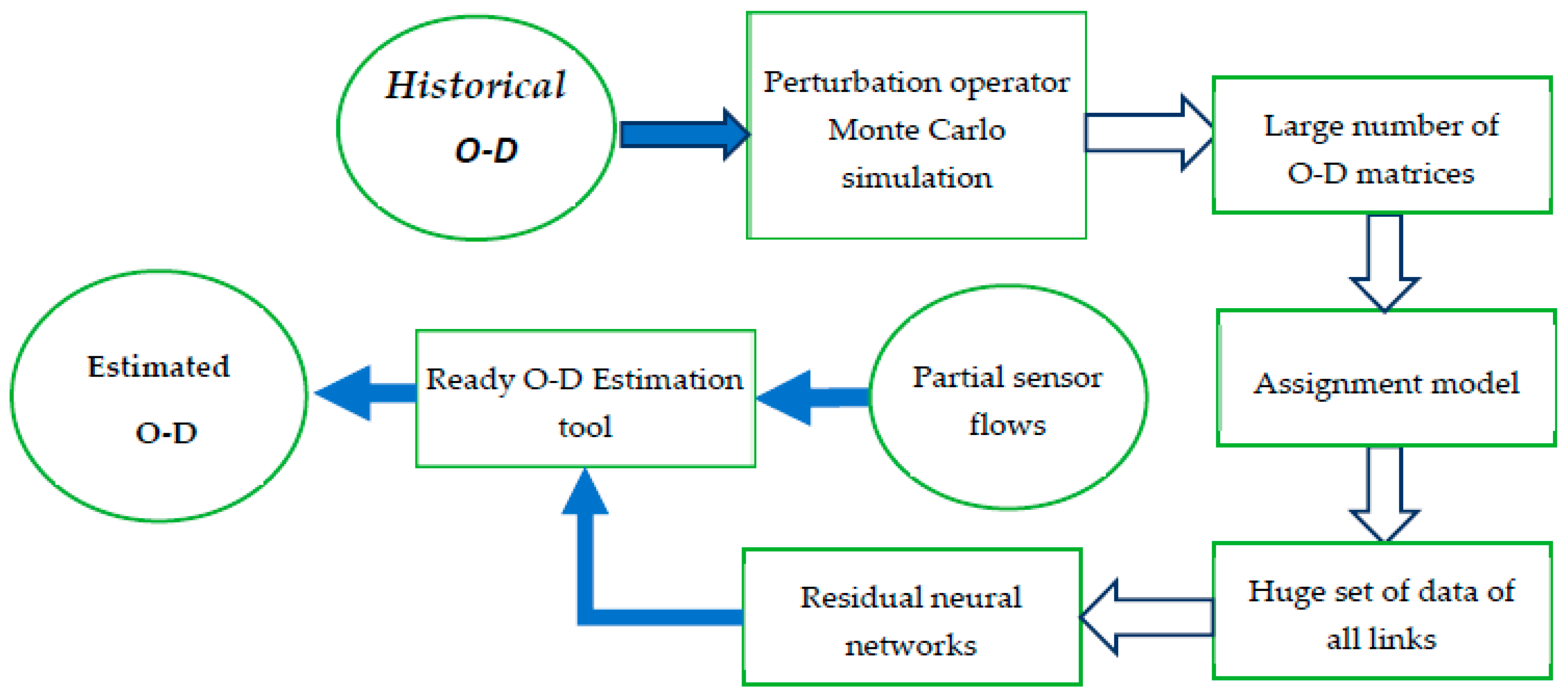
ML is a programming tool that enables one to make rational decisions based on learning data. The central concept of the proposed methodology is the belief that each network traffic flow results from a certain behavior considering its topology and demand level. This makes a strong correlation among traffic flow elements. If good sampling data are provided, the ML learns the behavior in the network and consequently predicts the full network flow from a number of observations. The general framework of the methodology is shown in Figure 2.
The essential premise of the suggested technique is that each transportation network flow originates from a common user’s response to the network’s structure and demand level. This demonstrates the presence of a substantial link between network structure and aspects of traffic flow. If we were able to gather adequate sample data, the defined ML algorithm would learn how the flow propagates and then estimate the O–D requirement from observed link flows.

4.1. Synthetic Input Data Generation

The genuine unknown demand, the reference/historical demand, and the anticipated demand (T*, T0, and T ¯ , respectively) might be accounted for in each ODEP. Each of these vectors has the same dimension. To target T*, total demand ( D ) is considered to be a random variable; hence, we may develop a space of demand vectors T, expressed as follows:
T = D P + γ
P = 1 µ D T 0
where D follows a normal distribution with an anticipated mean of µ D and a standard deviation of σ D . P = [ p w ] w ¯ × 1 is the vector of positive real values; p w represents the relative value of w to total demand D , as seen in Equation (15). γ is a vector of random variables with a mean of zero and a standard deviation of γ w [12,24]. Equations (14) and (15) are presented in this style so that they can reflect both the independent and correlated stochasticity in T.
The sample set for training ST = {T1, T2, …, Ti, …, Tn} may now be created using simulations based on the Monte Carlo algorithm. To prepare the data for the supervised learning stage, the assignment model is invoked to produce the relevant link flow vectors SX = {X1, X2, …, Xi, …, Xn}. The assignment formula in Equations (6)–(8) may be solved using Algorithm 1.
Algorithm 1: The DRNNS complete Algorithm
   Pre-condition: connected network (G), non-empty T
   Post-condition: link flows X
   1.  
assign each flow t w to the collection of stochastic pathways with Dial’s technique (More information on Dial’s technique is found in [69]), resulting in x a c t r flows on the links.
   2.  
set the counter (ctr=1).
   3.      
update ε a ( x a c t r ) = ε a 0 1 + α a ( x a c t r Q a ) χ a
   4.      
reassign t w to the new generated stochastic paths with ε a c t r , yielding x a c t r a set of auxiliary flows ( ω a c t r ).
   5.      
reassign t w to the newly produced stochastic routes with ε a c t r , to produce x a c t r set of auxiliary flows ( ω a c t r ).
   6.      
update x a c t r + 1 = x a c t r + q c t r ( ω a c t r x a c t r + 1 ), a A
   7.      
if a ( x a c t r + 1 x a c t r ) 2 a x a c t r κ go next, otherwise, set ctr:=ctr+1 and go step 3.
   8.  
return X = { x a c t r + 1 }
   9.  
end algorithm
Algorithm 1 provides the link flow vector X for the seeded demand vector T. It uses the method of successive averages (MSA) [70] as its basis. At the heart of the method, a search direction is formed at each iteration by allocating the flow to stochastic pathways based on the anticipated trip costs of the predecessor link flows. In comparable assignment algorithms, the step length q is adjusted in a number of ways to facilitate convergence [71]. In the MSA, the following step lengths sequence is utilized q c t r = 1/( c t r + 1 ).

4.2. Residual Neural Networks

This study uses the ResNet approach to build a new deep residual neural networks (DRNNs) model for the ODEP. Figure 3 illustrates the suggested DRNNs’ architecture. The construction of a DRNN consists of three primary portions: the starting, middle, and final sections, with a total of 34 levels. The first portion consists of an input layer, a convolution (Conv) layer, a batch normalization (BN) layer, and a rectified linear unit (ReLU) activation layer. The suggested architecture’s major portion, the center section, consists of a stack of four residual building units (ResBU). The last portion of the design consists of two layers: a fully connected (FC) layer and an output layer. The input layer is the initial foundation layer through which input data are standardized and provided to the system. The input data array is subtracted by its mean value and then divided by its variance during data normalization.
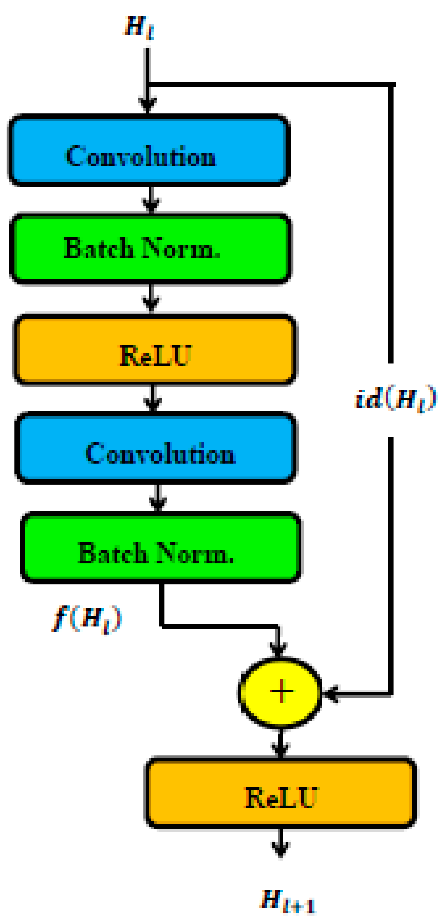
As shown in Figure 4, each residual building unit (ResBU) contains two branches: the main branch and the residual branch. Each Conv layer is followed by a BN and ReLU activation layer. The residual branch (shortcut connection) with the identity function of the input avoids the layers of the main branch. The residual branch output is added element-by-element to the main branch output shortly before the final ReLU activation layer. Each residual building unit (ResBU) executes the calculation described in Equation (13).
The existence of the shortcut link with the identity function smooths the gradient flow without introducing any additional computing complexity [72].
H l + 1 = R e L U f H l + i d H l
where H l , H l + 1 are the input and output of the lth residual building unit, respectively. f H l represents the residual function to be learned; i d H l represents the identity function; and l denotes the number of residual building units. After elementwise addition, ReLU is a rectified linear unit activation function.
In the construction of DRNNs, each Conv layer is followed by a BN layer and then a ReLU activation layer. Using a series of learnable kernels (filters) that extract local features from the input data, the convolution (Conv) layer can acquire a useful internal representation of the input data. As its name indicates, the convolution layer convolutes incoming data by sliding kernels along it. Each kernel creates a feature map by multiplying the input and associated weight by a bias value [73]. A batch normalization (BN) layer is allocated the output of the Conv layer. The BN layer is a potent regularization method that is primarily employed to prevent data overfitting [74].
In addition, by recentering and rescaling each input channel, the BN layer minimizes initialization sensitivity and accelerates the training process [75]. It begins by calculating a normalized activation of the input every minibatch and then scales and shifts it. The normalized activations are computed as follows:
x i ^ = x i μ B σ B 2 +
In addition, scaling and shifting the normalized activation is accomplished as follows [75]:
y i = γ x i ^ + β
where x i is the batch input; μ B and σ B 2 are the mean and variance of the minibatch, respectively; ϵ is a characteristic of epsilon that is utilized to improve numerical stability with low minibatch variance value. γ and β represent the scale and offset attributes, respectively (i.e., learnable and updated parameters through network training).
The output of the BN layer is assigned to a nonlinear activation layer (ReLU) that embeds nonlinearity into the network and hence facilitates the learning of complicated abstractions [76]. As seen below, the ReLU activation layer acts as a “decision function” to eliminate any negative values in the input ( y i ).
ReLU y i = max 0 , y i
In Equation (19), the ReLU beats various activation functions, including the saturating hyperbolic tang and sigmoid functions. ReLU makes training deep networks far quicker than other activation functions without compromising generalization accuracy [53,77].
The fully connected (FC) layer, the final layer in the hierarchy of DRNNs prior to the output layer, is used for prediction. Every neuron in the FC layer is linked to every neuron in the preceding layer. The FC layer collects all previously learned characteristics for the most accurate prediction [56]. The output layer, the last layer in the design of DRNNs, is a regression layer that computes the mean squared error (MSE) and loss function (Loss) for the ODEP.

4.3. Sensor Location Strategy

Although the selection technique is subjective in all reviewed design methodologies, there is no quality assurance for the predicted O–D matrix before the actual deployment of sensors in the network. In addition, there is a clear contradiction between the needed precision and the installation cost of the sensors. The suggested strategy for the solution to the TSLP seeks the number and placements of sensors that minimize the maximum relative error boundary for the estimated O–D matrix. The location problem for traffic sensors is phrased as a set coverage problem, and then a multicriteria metaheuristics approach is utilized. This method directly targets the largest potential relative error in the multi-objective design process, which is a robust criterion for assessing a solution set.
The suggested approach is predicated on a robust estimate of the possible accuracy of the ODEP in relation to the number of sensors employed. Set covering formulation is used to describe the problem of picking sensors (SCP). For this method, a new multicriteria metaheuristics method is adapted.
As mentioned before, the MPRE specifies that the amount of space permitted by traffic counts for a specifically fitted O–D matrix when this basis is assessed based on the maximum value of a quadratic index [14]. The MPRE is a reliable method for assessing the precision of observations originating from a sensor-equipped link set. To the best of our knowledge, no study in the literature determines the position of sensors based on the MPRE value except in [1] and the extension in [13].
Now, the TSLP solution is considered as solving the SCP, which is described as the issue of covering all rows of matrix at the lowest cost [78]. Any known integer solver could precisely solve the SCP, but it would not be advantageous for our case. This is due to two fundamental reasons: (1) it is categorized as NP-hard, meaning that it is difficult (impossible) to solve for real-scale networks (our aim) [79,80]; and (2) the best solution for the SCP does not always imply the optimal solution for the TSLP. Consequently, we recalled the metaheuristic presented in [1] to regulate the solution process and lead it towards the desired analysis. The algorithm details are illustrated in [12].

5. Numerical Study

This section illustrates how the approach provided may be used for large-scale networks. To assess the efficacy of the suggested method, a 900-node grid network was built. The network consists of 900 nodes and 3,480 links. The connecting journey times are a minute long. It has a respectable arc-to-node ratio of 3.87, despite the fact that the great majority of synthetically constructed extensive networks in the literature have values as high as 10 [81]. The network’s vertices consist of around 810,000 node pairs. It is impractical to regard all of these pairings of nodes as O–D pairs. Figure 5 depicts the correlation between the number of demand pairs and the number of links necessary to produce the lowest MPRE.
We selected the ten thousand couples with D S 1% for the remainder of the analysis to randomly produce the seeded O–D data with values ranging from 0 to 120 units/hour. The root mean square relative error (RMSE) or simply (RE) was picked as a performance indicator for the anticipated traffic flow created by the proposed architecture. RE evaluates the divergence from anticipated values as follows:
R E = w = 1 ŵ ( t w t r u e t w e s t . t w t r u e ) 2 w ¯
where t w t r u e represents the seeded Ti values in the assignment phase, while t w e s t . is the correspondent DRNNs’ flow estimates.
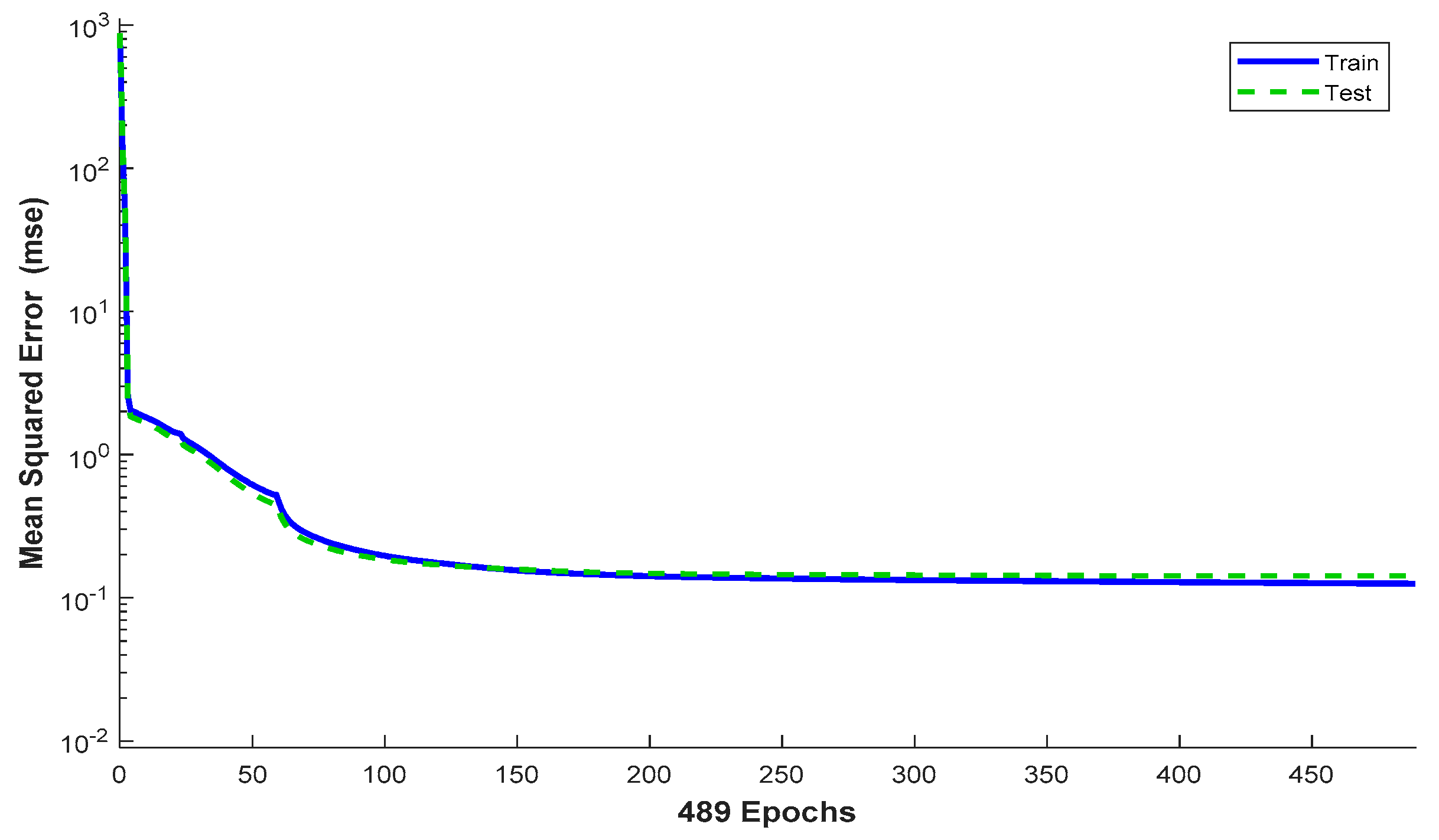
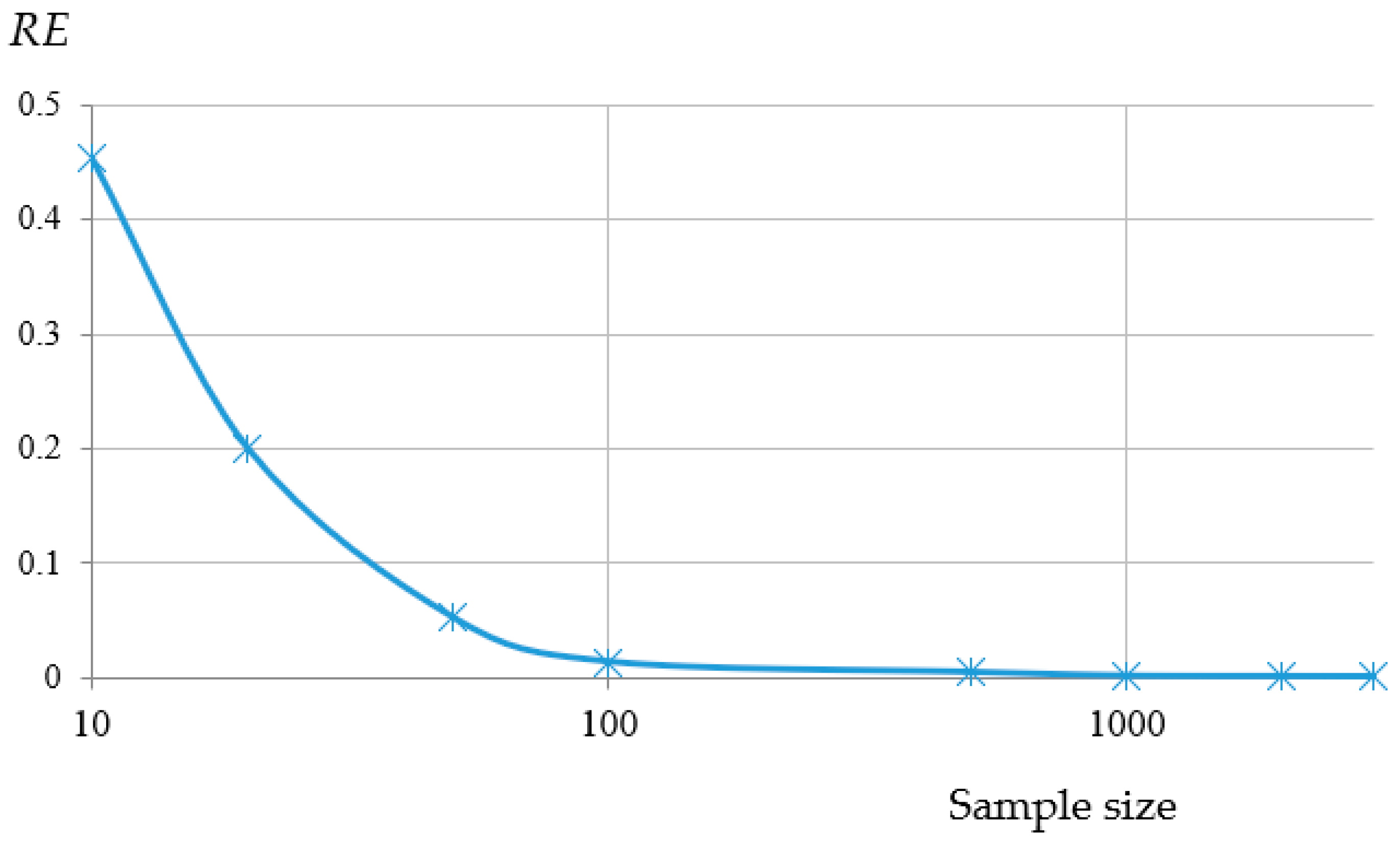
In the parameterization and training of the DRNNs model, 30 kernels of size 4 were used in each Conv layer to create 30 feature maps. The minibatch size for the stochastic gradient descent (SGD) was 256. For weight initialization, we employed the approach described in [82], which is suitable for DL networks with a ReLU activation layer. The DRNNs model was trained for one thousand iterations. The starting learning rate was set at 0.01 and subsequently decayed exponentially over 1000 epochs to 0.0001. We adjusted the settings for weight decay and momentum to 0.0001 and 0.90, respectively. The entire DRNN architecture was implemented using MATLAB 2020a software running on a workstation with a 2.3 GHz Intel® Xeon® CPU, 16 GB of RAM, and a GeForce GTX 1060 graphics card. The efficiency of the model is depicted in Figure 6. In Figure 7, the influence of sample size on accuracy is examined, given that every ML approach requires a sufficient number of points to achieve the necessary learning. The RE value converged at a demand vector sample size of 1000.
Inputs and outputs of the database were normalized for the suggested DRNNs structure, and then the data set was randomly separated into two groups, training and testing. Eighty percent of the implemented database’s 732,000 data points were utilized for training, while the remaining twenty percent were used for testing. Figure 8 illustrates the seeded-predicted plot for each O–D combination, with the best-fitting line compared to the line of equality (LOE) to illustrate how well predictions matched seeded data. Four subplots ((a) to (d)) convey the performance through training, validation, testing, and all data cases. The DRNNs accurately predicted the demand flow value, which conveys the methodology’s credibility.
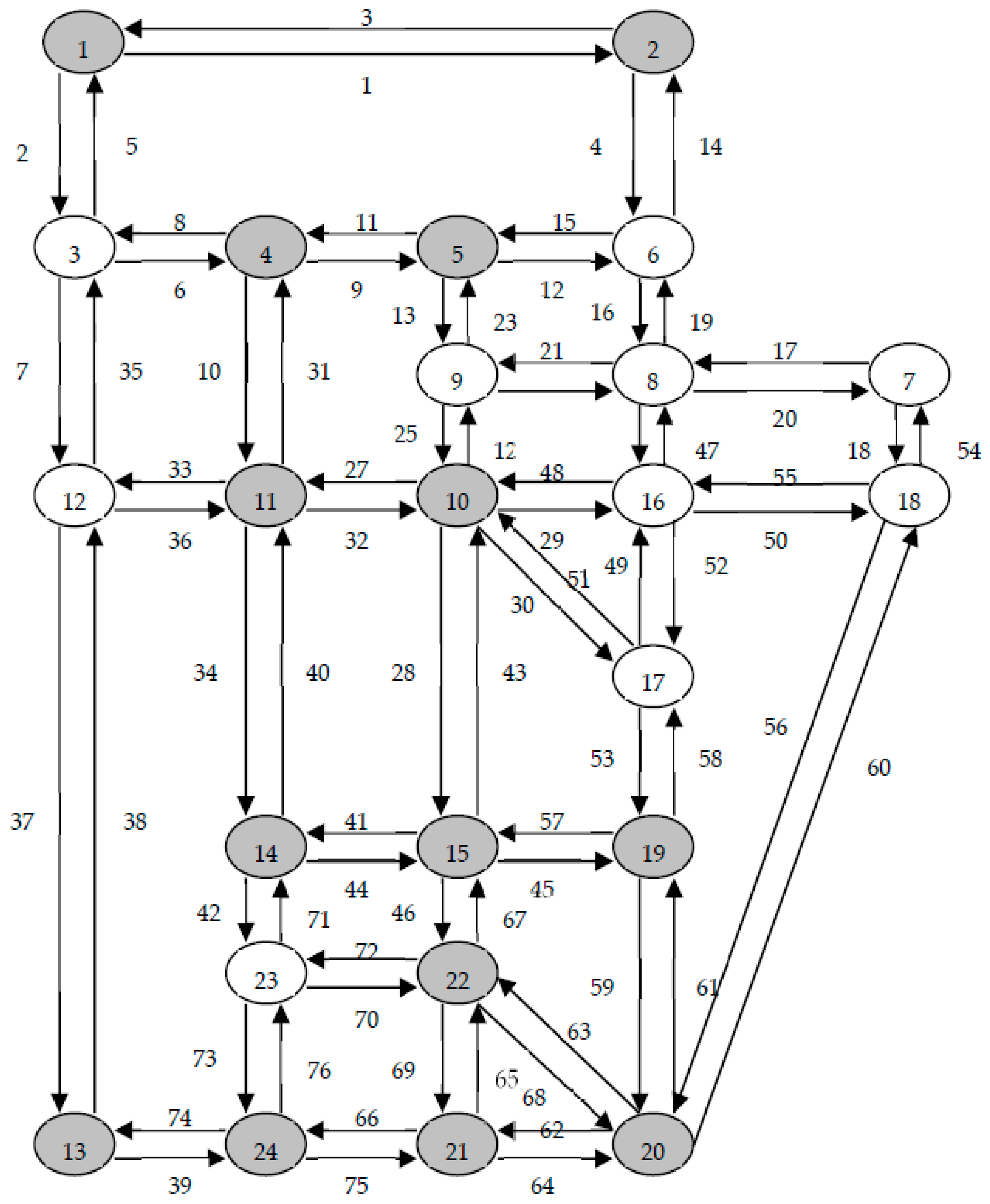
The second network used in this study is also a well-documented medium network with 76 connections, 182 O/D pairs, and 24 nodes; refer to Figure 9, where the shaded nodes indicate both trip origins/destinations and the link coding numbers are provided. The network was initially proposed in [23] for the TSLP issue. It is a benchmark problem in the majority of the TSLP literature [7,11,23,83,84,85,86,87,88,89,90,91]. Using the Sioux Falls network reference demand provided by [24] together with γ w = 0.25 t w 0 , the objective of this phase was to validate the performance of the entire suggested technique utilizing a real network that contained not only the reference demand data, but also the entire genuine set. In other words, the training data and validation data were distinct. Despite the fact that this scenario does not exist in the actual world, it illustrates the genuine estimation accuracy of the process. While the reference demand of the network was utilized for training, the actual demand was used for validation. Table 2 compares the presented methodology with different studies from the literature that solved the TSLP targeting ODE problem. It is clear that the DRNNs achieved superior accuracy due to their outstanding ability to learn the inherent relationship between synthetically generated data and assigned link flows. Figure 10 reflects the effect of sensor number on the obtained accuracy. It constitutes the Pareto optimal solution that allows the analyst to choose the suitable sensor number according to the available budget and required accuracy.

6. Conclusions

This work introduced a new contribution to the ODEP based on an exhaustive literature assessment. Deploying sensors on all network links is impractical, and it is tough to translate passive link counts into O–D flow data. These are the two primary causes of the aforementioned combined problem difficulties. The analyzed condition is the installation of traffic-counting sensors on network lines that produce the most precise O–D prediction utilizing DRNN architecture. In addition, a simulation environment for the DRNNs’ training may be easily obtained by assuming the correct traffic assignment model assumptions. The proposed DRNNs model’s objective was to identify the concealed O–D flow characteristics. This may allow for the creation of major O–D and link flow patterns. In addition, the model can originate solutions that are close to the optimal solution or attain much superior local minima, hence decreasing convergence time. The FCL was then included in the O–D estimate. Lastly, a well-cited sensor location strategy from the literature was used to investigate the relevance of the links in the TSLP’s prediction phase. The numerical findings demonstrate that the technique may achieve accuracy, with large-scale networks reaching 97 percent. At the same time, the methodology managed to surpass other methods from the literature by achieving 99 percent accuracy with only 20 sensors. Observational errors should be addressed in future studies, as they occur in practically all practical applications. Due to the fact that defects may cause a variety of issues, several correction steps are necessary. Few articles have investigated the potential of information noise utilizing the two major themes of measurement error and complete sensor failure. The former focuses on limiting the propagation of measurement mistakes while considering error variations during the solution process. Considering the likelihood of sensor failure, the latter strategy aims to ensure minimal flow information loss. Considering the fact that observational mistakes are not the primary subject of this article, the topic needs its own investigation due to its unique contribution. It would be a new challenge for ML to concurrently handle the two sorts of uncertainty (i.e., sensor errors and seeded demand fluctuations).

Author Contributions

Conceptualization, M.O.; Data curation, A.A. and M.H.A.; Formal analysis, M.O. and J.G.; Funding acquisition, A.A.; Investigation, S.A.; Methodology, M.O.; Project administration, A.A.; Resources, A.A. and S.A.; Software, J.G.; Supervision, S.A.; Validation, M.O. and M.H.A.; Visualization, J.G.; Writing—original draft, M.O.; Writing—review and editing, M.H.A. All authors have read and agreed to the published version of the manuscript.

Funding

This research was funded by The Deputyship For Research and Innovation, grant number IFP-2022-30.

Institutional Review Board Statement

Not applicable.

Informed Consent Statement

Not applicable.

Data Availability Statement

The data files related to this research are available upon request from the corresponding author, Mahmoud Owais.

Acknowledgments

The authors extend their appreciation to Research and Innovation, Ministry Education of Saudi Arabia for funding this research work through project number (IFP-2022-30).

Conflicts of Interest

The authors declare no conflict of interest.

References

  1. Owais, M.; Moussa, G.S.; Hussain, K.F. Sensor location model for O/D estimation: Multi-criteria meta-heuristics approach. Oper. Res. Perspect. 2019, 6, 100100. [Google Scholar] [CrossRef]
  2. Owais, M.; Matouk, A.E. A factorization scheme for observability analysis in transportation networks. Expert Syst. Appl. 2021, 174, 114727. [Google Scholar] [CrossRef]
  3. Nie, Y.; Zhang, H.; Lee, D.-H. Models and algorithms for the traffic assignment problem with link capacity constraints. Transp. Res. Part B Methodol. 2004, 38, 285–312. [Google Scholar] [CrossRef]
  4. Owais, M. Location Strategy for Traffic Emission Remote Sensing Monitors to Capture the Violated Emissions. J. Adv. Transp. 2019, 2019, 6520818. [Google Scholar] [CrossRef] [Green Version]
  5. Chen, A.; Chootinan, P.; Ryu, S.; Wong, S.C. Quality Measures of Origin-Destination Trip Table Estimated from Traffic Counts: Review and New Generalized Demand Scale Measure. J. Transp. Eng. 2012, 138, 1340–1349. [Google Scholar] [CrossRef]
  6. Bianco, L.; Confessore, G.; Reverberi, P. A Network Based Model for Traffic Sensor Location with Implications on O/D Matrix Estimates. Transp. Sci. 2001, 35, 50–60. [Google Scholar] [CrossRef]
  7. Yang, C.; Chootinan, P.; Chen, A. Traffic counting location planning using genetic algorithm. J. East. Asia Soc. Transp. Stud. 2003, 5, 898–913. [Google Scholar]
  8. Owais, M. Traffic Sensor Location Problem: Three Decades of Research. Expert Syst. Appl. 2022, 208, 118134. [Google Scholar] [CrossRef]
  9. Owais, M.; El deeb, M.; Abbas, Y.A. Distributing Portable Excess Speed Detectors in AL Riyadh City. Int. J. Civ. Eng. 2020, 18, 1301–1314. [Google Scholar] [CrossRef]
  10. Gentili, M.; Mirchandani, P.B. Locating sensors on traffic networks: Models, challenges and research opportunities. Transp. Res. Part C Emerg. Technol. 2012, 24, 227–255. [Google Scholar] [CrossRef]
  11. Fu, C.; Zhu, N.; Ling, S.; Ma, S.; Huang, Y. Heterogeneous sensor location model for path reconstruction. Transp. Res. Part B Methodol. 2016, 91, 77–97. [Google Scholar] [CrossRef]
  12. Owais, M.; Shahin, A.I. Exact and Heuristics Algorithms for Screen Line Problem in Large Size Networks: Shortest Path-Based Column Generation Approach. IEEE Trans. Intell. Transp. Syst. 2022, 23, 24829–24840. [Google Scholar] [CrossRef]
  13. Salari, M.; Kattan, L.; Lam, W.H.; Esfeh, M.A.; Fu, H. Modeling the effect of sensor failure on the location of counting sensors for origin-destination (OD) estimation. Transp. Res. Part C Emerg. Technol. 2021, 132, 103367. [Google Scholar] [CrossRef]
  14. Yang, H.; Iida, Y.; Sasaki, T. An analysis of the reliability of an origin-destination trip matrix estimated from traffic counts. Transp. Res. Part B Methodol. 1991, 25, 351–363. [Google Scholar] [CrossRef]
  15. Antoniou, C.; Barceló, J.; Breen, M.; Bullejos, M.; Casas, J.; Cipriani, E.; Ciuffo, B.; Djukic, T.; Hoogendoorn, S.; Marzano, V. Towards a generic benchmarking platform for origin–destination flows estimation/updating algorithms: Design, demonstration and validation. Transp. Res. Part C Emerg. Technol. 2016, 66, 79–98. [Google Scholar] [CrossRef]
  16. Gaudry, M.; Lamarre, L. Estimating origin-destination matrices from traffic counts: A simple linear intercity model for Quebec. Logist. Transp. Rev. 1979, 15, 631–642. [Google Scholar]
  17. Lam, W.H.; Lo, H. Estimation of origin-destination matrix from traffic counts: A comparison of entropy maximizing and information minimizing models. Transp. Plan. Technol. 1991, 16, 85–104. [Google Scholar] [CrossRef]
  18. Cascetta, E. Estimation of trip matrices from traffic counts and survey data: A generalized least squares estimator. Transp. Res. Part B Methodol. 1984, 18, 289–299. [Google Scholar] [CrossRef]
  19. Spiess, H. A maximum likelihood model for estimating origin-destination matrices. Transp. Res. Part B Methodol. 1987, 21, 395–412. [Google Scholar] [CrossRef]
  20. Castillo, E.; Menéndez, J.M.; Sánchez-Cambronero, S. Predicting traffic flow using Bayesian networks. Transp. Res. Part B Methodol. 2008, 42, 482–509. [Google Scholar] [CrossRef]
  21. Castillo, E.; Menéndez, J.M.; Sánchez-Cambronero, S. Traffic estimation and optimal counting location without path enumeration using Bayesian networks. Comput.-Aided Civ. Infrastruct. Eng. 2008, 23, 189–207. [Google Scholar] [CrossRef]
  22. Gentili, M.; Mirchandani, P.B. Locating active sensors on traffic networks. Ann. Oper. Res. 2005, 136, 229–257. [Google Scholar] [CrossRef]
  23. Yang, H.; Zhou, J. Optimal traffic counting locations for origin–destination matrix estimation. Transp. Res. Part B Methodol. 1998, 32, 109–126. [Google Scholar] [CrossRef]
  24. Ehlert, A.; Bell, M.G.H.; Grosso, S. The optimisation of traffic count locations in road networks. Transp. Res. Part B Methodol. 2006, 40, 460–479. [Google Scholar] [CrossRef]
  25. Bierlaire, M. The total demand scale: A new measure of quality for static and dynamic origin–destination trip tables. Transp. Res. Part B Methodol. 2002, 36, 837–850. [Google Scholar] [CrossRef]
  26. Yang, H. Heuristic algorithms for the bilevel origin-destination matrix estimation problem. Transp. Res. Part B Methodol. 1995, 29, 231–242. [Google Scholar] [CrossRef]
  27. Maher, M.J.; Zhang, X.; Van Vliet, D. A bi-level programming approach for trip matrix estimation and traffic control problems with stochastic user equilibrium link flows. Transp. Res. Part B Methodol. 2001, 35, 23–40. [Google Scholar] [CrossRef] [Green Version]
  28. Maher, M.; Zhang, X. Algorithms for the solution of the congested trip matrix estimation problem. In Proceedings of the 14th International Symposium on Transportation and Traffic Theory, Jerusalem, Israel, 20–23 July 1999. [Google Scholar]
  29. Lo, H.-P.; Chan, C.-P. Simultaneous estimation of an origin–destination matrix and link choice proportions using traffic counts. Transp. Res. Part A Policy Pract. 2003, 37, 771–788. [Google Scholar] [CrossRef]
  30. Han, Z.; Yang, Y.; Wang, W.; Zhou, L.; Nguyen, T.N.; Su, C. Age Efficient Optimization in UAV-Aided VEC Network: A Game Theory Viewpoint. IEEE Trans. Intell. Transp. Syst. 2022, 23, 25287–25296. [Google Scholar] [CrossRef]
  31. Bell, M.G.; Shield, C.M. A log-linear model for path flow estimation. In Proceedings of the Applications of Advanced Technologies in Transportation Engineering, Capri, Italy, 27–30 June 1995; pp. 695–699. [Google Scholar]
  32. Bell, M.G.; Shield, C.M.; Busch, F.; Kruse, G. A stochastic user equilibrium path flow estimator. Transp. Res. Part C Emerg. Technol. 1997, 5, 197–210. [Google Scholar] [CrossRef]
  33. Nie, Y.; Zhang, H.; Recker, W. Inferring origin–destination trip matrices with a decoupled GLS path flow estimator. Transp. Res. Part B Methodol. 2005, 39, 497–518. [Google Scholar] [CrossRef]
  34. Nie, Y.; Lee, D.-H. Uncoupled method for equilibrium-based linear path flow estimator for origin-destination trip matrices. Transp. Res. Rec. J. Transp. Res. Board 2002, 1783, 72–79. [Google Scholar] [CrossRef]
  35. Chootinan, P.; Chen, A.; Recker, W. Improved path flow estimator for origin-destination trip tables. Transp. Res. Rec. J. Transp. Res. Board 2005, 1923, 9–17. [Google Scholar] [CrossRef]
  36. Chen, A.; Ryu, S.; Chootinan, P. L∞-norm path flow estimator for handling traffic count inconsistencies: Formulation and solution algorithm. J. Transp. Eng. 2010, 136, 565–575. [Google Scholar] [CrossRef]
  37. Maher, M. Inferences on trip matrices from observations on link volumes: A Bayesian statistical approach. Transp. Res. Part B Methodol. 1983, 17, 435–447. [Google Scholar] [CrossRef]
  38. Wei, C.; Asakura, Y. A Bayesian approach to traffic estimation in stochastic user equilibrium networks. Transp. Res. Part C Emerg. Technol. 2013, 36, 446–459. [Google Scholar] [CrossRef]
  39. Castillo, E.; Conejo, A.J.; Menéndez, J.M.; Jimenez, P. The observability problem in traffic network models. Comput.-Aided Civ. Infrastruct. Eng. 2008, 23, 208–222. [Google Scholar] [CrossRef]
  40. Castillo, E.; Jiménez, P.; Menéndez, J.M.; Conejo, A.J. The observability problem in traffic models: Algebraic and topological methods. Intell. Transp. Syst. IEEE Trans. 2008, 9, 275–287. [Google Scholar] [CrossRef]
  41. Castillo, E.; Gallego, I.; Sanchez-Cambronero, S.; Rivas, A. Matrix tools for general observability analysis in traffic networks. IEEE Trans. Intell. Transp. Syst. 2010, 11, 799–813. [Google Scholar] [CrossRef]
  42. Chen, A.; Pravinvongvuth, S.; Chootinan, P.; Lee, M.; Recker, W. Strategies for selecting additional traffic counts for improving OD trip table estimation. Transportmetrica 2007, 3, 191–211. [Google Scholar] [CrossRef]
  43. Fei, X.; Mahmassani, H.; Eisenman, S. Sensor coverage and location for real-time traffic prediction in large-scale networks. Transp. Res. Rec. J. Transp. Res. Board 2007, 2039, 1–15. [Google Scholar] [CrossRef] [Green Version]
  44. Fei, X.; Mahmassani, H.S. Structural analysis of near-optimal sensor locations for a stochastic large-scale network. Transp. Res. Part C Emerg. Technol. 2011, 19, 440–453. [Google Scholar] [CrossRef]
  45. Goswami, S.; Kumar, A. Traffic Flow Prediction Using Deep Learning Techniques. In Proceedings of the International Conference on Computing Science, Communication and Security, Gujarat, India, 6–7 February 2022; pp. 198–213. [Google Scholar]
  46. Lv, Y.; Duan, Y.; Kang, W.; Li, Z.; Wang, F.-Y. Traffic flow prediction with big data: A deep learning approach. IEEE Trans. Intell. Transp. Syst. 2014, 16, 865–873. [Google Scholar] [CrossRef]
  47. Yin, X.; Wu, G.; Wei, J.; Shen, Y.; Qi, H.; Yin, B. Deep learning on traffic prediction: Methods, analysis and future directions. IEEE Trans. Intell. Transp. Syst. 2021, 23, 4927–4943. [Google Scholar] [CrossRef]
  48. Guo, K.; Hu, Y.; Qian, Z.; Liu, H.; Zhang, K.; Sun, Y.; Gao, J.; Yin, B. Optimized graph convolution recurrent neural network for traffic prediction. IEEE Trans. Intell. Transp. Syst. 2020, 22, 1138–1149. [Google Scholar] [CrossRef]
  49. Ou, J.; Lu, J.; Xia, J.; An, C.; Lu, Z. Learn, assign, and search: Real-time estimation of dynamic origin-destination flows using machine learning algorithms. IEEE Access 2019, 7, 26967–26983. [Google Scholar] [CrossRef]
  50. Rao, W.; Wu, Y.-J.; Xia, J.; Ou, J.; Kluger, R. Origin-destination pattern estimation based on trajectory reconstruction using automatic license plate recognition data. Transp. Res. Part C Emerg. Technol. 2018, 95, 29–46. [Google Scholar] [CrossRef]
  51. Tang, K.; Cao, Y.; Chen, C.; Yao, J.; Tan, C.; Sun, J. Dynamic origin-destination flow estimation using automatic vehicle identification data: A 3D convolutional neural network approach. Comput.-Aided Civ. Infrastruct. Eng. 2021, 36, 30–46. [Google Scholar] [CrossRef]
  52. Wang, Q.; Yuan, Y.; Zhang, Q.; Yang, X.T. Signalized arterial origin-destination flow estimation using flawed vehicle trajectories: A self-supervised learning approach without ground truth. Transp. Res. Part C Emerg. Technol. 2022, 145, 103917. [Google Scholar] [CrossRef]
  53. Li, J.; Boonaert, J.; Doniec, A.; Lozenguez, G. Multi-models machine learning methods for traffic flow estimation from Floating Car Data. Transp. Res. Part C Emerg. Technol. 2021, 132, 103389. [Google Scholar] [CrossRef]
  54. Elhenawy, M.; Rakha, H. Spatiotemporal traffic state prediction based on discriminatively pre-trained deep neural networks. Adv. Sci. Technol. Eng. Syst. 2017, 2, 678–686. [Google Scholar] [CrossRef] [Green Version]
  55. Karantaglis, N.; Passalis, N.; Tefas, A. Predicting on-street parking violation rate using deep residual neural networks. Pattern Recognit. Lett. 2022, 163, 82–91. [Google Scholar] [CrossRef]
  56. Moussa, G.S.; Owais, M.; Dabbour, E. Variance-based global sensitivity analysis for rear-end crash investigation using deep learning. Accid. Anal. Prev. 2022, 165, 106514. [Google Scholar] [CrossRef] [PubMed]
  57. Castillo, E.; Jiménez, P.; Menéndez, J.M.; Nogal, M. A Bayesian method for estimating traffic flows based on plate scanning. Transportation 2013, 40, 173–201. [Google Scholar] [CrossRef]
  58. Bell, M.G. The estimation of an origin-destination matrix from traffic counts. Transp. Sci. 1983, 17, 198–217. [Google Scholar] [CrossRef]
  59. Wang, W.; Srivastava, G.; Lin, J.C.-W.; Yang, Y.; Alazab, M.; Gadekallu, T.R. Data freshness optimization under CAA in the UAV-aided MECN: A potential game perspective. IEEE Trans. Intell. Transp. Syst. 2022, 1–10. [Google Scholar] [CrossRef]
  60. Wang, J.; Peeta, S.; He, X. Multiclass traffic assignment model for mixed traffic flow of human-driven vehicles and connected and autonomous vehicles. Transp. Res. Part B Methodol. 2019, 126, 139–168. [Google Scholar] [CrossRef]
  61. Owais, M.; Osman, M.K. Complete hierarchical multi-objective genetic algorithm for transit network design problem. Expert Syst. Appl. 2018, 114, 143–154. [Google Scholar] [CrossRef]
  62. Owais, M.; Hassan, T. Incorporating dynamic bus stop simulation into static transit assignment models. Int. J. Civ. Eng. 2018, 16, 67–77. [Google Scholar] [CrossRef]
  63. Owais, M.; Ahmed, A.S. Frequency Based Transit Assignment Models: Graph Formulation Study. IEEE Access 2022, 10, 62991–63003. [Google Scholar] [CrossRef]
  64. Batista, S.F.; Leclercq, L. Regional dynamic traffic assignment framework for macroscopic fundamental diagram multi-regions models. Transp. Sci. 2019, 53, 1563–1590. [Google Scholar] [CrossRef]
  65. Owais, M.; Ahmed, A.S.; Moussa, G.S.; Khalil, A.A. An optimal metro design for transit networks in existing square cities based on non-demand criterion. Sustainability 2020, 12, 9566. [Google Scholar] [CrossRef]
  66. Zhang, X.; Liu, W.; Waller, S.T. A network traffic assignment model for autonomous vehicles with parking choices. Comput.-Aided Civ. Infrastruct. Eng. 2019, 34, 1100–1118. [Google Scholar] [CrossRef]
  67. Spiess, H. Technical note—Conical volume-delay functions. Transp. Sci. 1990, 24, 153–158. [Google Scholar] [CrossRef] [Green Version]
  68. Owais, M.; Abulwafa, O.; Abbas, Y.A. When to decide to convert a roundabout to a signalized intersection: Simulation approach for case studies in Jeddah and Al-Madinah. Arab. J. Sci. Eng. 2020, 45, 7897–7914. [Google Scholar] [CrossRef]
  69. Fisk, C. Some developments in equilibrium traffic assignment. Transp. Res. Part B Methodol. 1980, 14, 243–255. [Google Scholar] [CrossRef]
  70. Powell, W.B.; Sheffi, Y. The convergence of equilibrium algorithms with predetermined step sizes. Transp. Sci. 1982, 16, 45–55. [Google Scholar] [CrossRef]
  71. Maher, M. Algorithms for logit-based stochastic user equilibrium assignment. Transp. Res. Part B Methodol. 1998, 32, 539–549. [Google Scholar] [CrossRef]
  72. He, K.; Zhang, X.; Ren, S.; Sun, J. Deep residual learning for image recognition. In Proceedings of the IEEE Conference on Computer Vision and Pattern Recognition, Las Vegas, NV, USA, 26 June–1 July 2016; pp. 770–778. [Google Scholar]
  73. Zang, J.; Wang, L.; Liu, Z.; Zhang, Q.; Hua, G.; Zheng, N. Attention-based temporal weighted convolutional neural network for action recognition. In Proceedings of the IFIP International Conference on Artificial Intelligence Applications and Innovations, Rhodes, Greece, 25–27 May 2018; pp. 97–108. [Google Scholar]
  74. Ioffe, S.; Szegedy, C. Batch normalization: Accelerating deep network training by reducing internal covariate shift. arXiv 2015, arXiv:1502.03167. [Google Scholar]
  75. Goodfelow, I.; Bengio, Y.; Courville, A. Deep Learning (Adaptive Computation and Machine Learning Series); The MIT Press: Cambridge, UK, 2016. [Google Scholar]
  76. Szegedy, C.; Liu, W.; Jia, Y.; Sermanet, P.; Reed, S.; Anguelov, D.; Erhan, D.; Vanhoucke, V.; Rabinovich, A. Going deeper with convolutions. In Proceedings of the IEEE Conference on Computer Vision and Pattern Recognition, Boston, MA, USA, 7–12 June 2015; pp. 1–9. [Google Scholar]
  77. Wang, W.; Han, Z.; Alazab, M.; Gadekallu, T.R.; Zhou, X.; Su, C. Ultra super fast authentication protocol for electric vehicle charging using extended chaotic maps. IEEE Trans. Ind. Appl. 2022, 58, 5616–5623. [Google Scholar] [CrossRef]
  78. Beasley, J.E.; Chu, P.C. A genetic algorithm for the set covering problem. Eur. J. Oper. Res. 1996, 94, 392–404. [Google Scholar] [CrossRef]
  79. Chvatal, V. A greedy heuristic for the set-covering problem. Math. Oper. Res. 1979, 4, 233–235. [Google Scholar] [CrossRef]
  80. Lan, G.; DePuy, G.W.; Whitehouse, G.E. An effective and simple heuristic for the set covering problem. Eur. J. Oper. Res. 2007, 176, 1387–1403. [Google Scholar] [CrossRef]
  81. Zhan, F.B.; Noon, C.E. Shortest path algorithms: An evaluation using real road networks. Transp. Sci. 1998, 32, 65–73. [Google Scholar] [CrossRef] [Green Version]
  82. He, K.; Zhang, X.; Ren, S.; Sun, J. Delving deep into rectifiers: Surpassing human-level performance on imagenet classification. In Proceedings of the IEEE International Conference on Computer Vision, Santiago, Chile, 7–13 December 2015; pp. 1026–1034. [Google Scholar]
  83. Yang, H.; Gan, L.; Tang, W. Determing cordons and screen lines for origin-destination trip studies. In Proceedings of the Eastern Asia Society for Transportation Studies, Hanoi, Vietnam, 23–27 October 2001; Volume 3. [Google Scholar]
  84. Chen, A.; Chootinan, P.; Recker, W.W. Examining the quality of synthetic origin–destination trip table estimated by path flow estimator. J. Transp. Eng. 2005, 131, 506–513. [Google Scholar] [CrossRef]
  85. Chootinan, P.; Chen, A.; Yang, H. A bi-objective traffic counting location problem for origin-destination trip table estimation. Transportmetrica 2005, 1, 65–80. [Google Scholar] [CrossRef]
  86. Hu, S.-R.; Peeta, S.; Chu, C.-H. Identification of vehicle sensor locations for link-based network traffic applications. Transp. Res. Part B Methodol. 2009, 43, 873–894. [Google Scholar] [CrossRef]
  87. Zangui, M.; Yin, Y.; Lawphongpanich, S. Sensor location problems in path-differentiated congestion pricing. Transp. Res. Part C Emerg. Technol. 2015, 55, 217–230. [Google Scholar] [CrossRef]
  88. He, S.-X. A graphical approach to identify sensor locations for link flow inference. Transp. Res. Part B Methodol. 2013, 51, 65–76. [Google Scholar] [CrossRef]
  89. Hadavi, M.; Shafahi, Y. Vehicle identification sensor models for origin–destination estimation. Transp. Res. Part B Methodol. 2016, 89, 82–106. [Google Scholar] [CrossRef]
  90. Xu, X.; Lo, H.K.; Chen, A.; Castillo, E. Robust network sensor location for complete link flow observability under uncertainty. Transp. Res. Part B Methodol. 2016, 88, 1–20. [Google Scholar] [CrossRef]
  91. Liu, Y.; Zhu, N.; Ma, S.; Jia, N. Traffic sensor location approach for flow inference. IET Intell. Transp. Syst. 2015, 9, 184–192. [Google Scholar] [CrossRef]
  92. Viti, F.; Cantelmo, G.; Corman, F.; Rinaldi, M. Improving the reliability of demand estimation using traffic counts by including information on link flow observability. In Proceedings of the 6th International Symposium on Transportation Network Reliability (INSTR 2015), Nara, Japan, 2–3 August 2015. [Google Scholar]
  93. Fu, H.; Lam, W.H.; Shao, H.; Xu, X.; Lo, H.; Chen, B.Y.; Sze, N.; Sumalee, A. Optimization of traffic count locations for estimation of travel demands with covariance between origin-destination flows. Transp. Res. Part C Emerg. Technol. 2019, 108, 49–73. [Google Scholar] [CrossRef]
  94. An, S.; Ma, L.; Wang, J. Optimization of traffic detector layout based on complex network theory. Sustainability 2020, 12, 2048. [Google Scholar] [CrossRef] [Green Version]
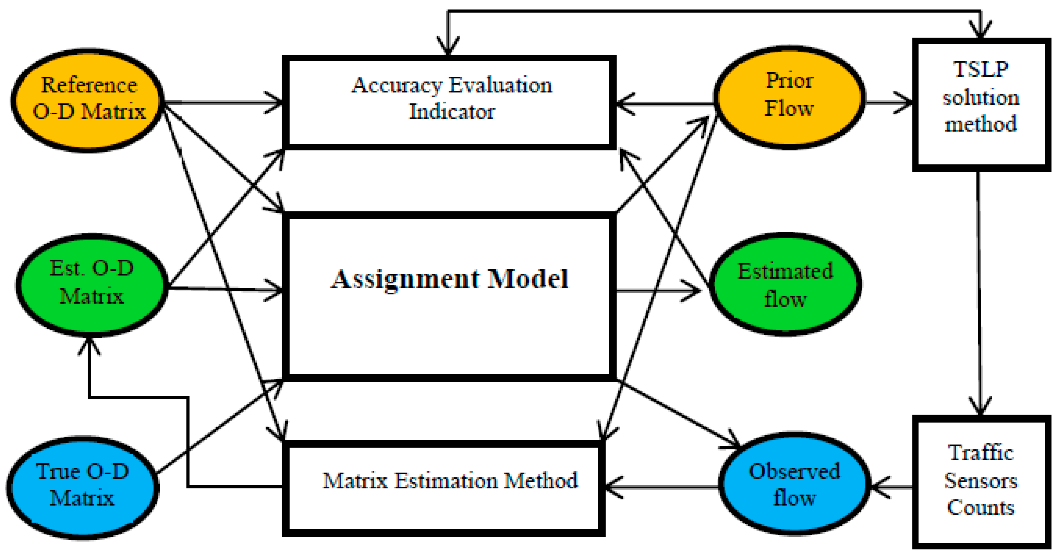
Figure 1. The relation among ODEP and TSLP input and output data.
Sustainability 15 09881 g001
Figure 2. The proposed framework to solve the ODEP.
Sustainability 15 09881 g002
Figure 3. Proposed architecture for the DRNNs.
Sustainability 15 09881 g003
Figure 4. The ResBU structure.
Sustainability 15 09881 g004
Figure 5. Number of required sensors vs. the number of O–D pairs created by the algorithm in [1].
Sustainability 15 09881 g005
Figure 6. DRNN curves of learning for training and testing data.
Sustainability 15 09881 g006
Figure 7. Effect of sample size on model prediction accuracy.
Sustainability 15 09881 g007
Figure 8. The DRNN performance evaluation based on the correlation coefficient.
Sustainability 15 09881 g008
Figure 9. Sioux Falls network structure.
Sustainability 15 09881 g009
Figure 10. Attained accuracy versus sensors number for Sioux Falls network.
Sustainability 15 09881 g010
Table 1. Transit assignment model choice variables.
AssumptionModel Choice DimensionsThis Study
Congestion effectAll or nothing Multipath Multipath
Equilibrium typeDeterministic StochasticStochastic
Capacity constraintMildStrictMild
Solution algorithmLink-basedPath-basedLink-based
Table 2. Sioux Falls comparison with the literature.
StudyYearNumber of SensorsTSLP MethodODE MethodSensors’ Uncertainty ConsiderationBest Reported Accuracy
F. Viti et al. [92]201515Greedy heuristicGeneralized least squaresno90%
Hao Fu, et al. [93]201911Firefly algorithmMaximum possible relative error for meanno88%
Owais, et al. [1]201920Random priority selection methodOrdinary least
square
no92%
Shi An, et al. [94]202010Complex networkTraffic network centrality modelyes95%
Mostafa Salari, et al. [13]202135Genetic algorithmMaximum possible information lossyesNot
reported
This study202320Random priority selection methodDRNNsno99%
Disclaimer/Publisher’s Note: The statements, opinions and data contained in all publications are solely those of the individual author(s) and contributor(s) and not of MDPI and/or the editor(s). MDPI and/or the editor(s) disclaim responsibility for any injury to people or property resulting from any ideas, methods, instructions or products referred to in the content.