Abstract
Load frequency control (LFC) serves as a crucial component of automatic generation control in renewable energy power systems. Its primary objective is to maintain a balance between the output power of generators and the load demand, thereby ensuring system frequency stability. However, integrating renewable energy sources into power systems brings forth several challenges, such as low power quality and poor system stability due to their uncontrollable nature. To enhance the response speed, stability, and disturbance rejection capabilities of LFC, a novel fractional-order active disturbance rejection controller (NFOADRC) based on an improved marine predator algorithm (IMPA) has been designed in this paper. By leveraging the wide frequency-response range and non-local memory of NFOADRC, a more precise prediction and compensation of rapid oscillations in the system can be achieved. Additionally, the IMPA can be utilized for efficient parameter tuning, enabling a more accurate adjustment of the controller. Subsequently, the combined application of these approaches can be applied to two-area interconnected power systems with a solar thermal power plant (STPP) and a five-area interconnected power system including a wind turbine generator (WTG), photovoltaic (PV) cells, hydro turbine, and gas turbine. The simulation results confirm that the proposed control strategy effectively minimizes the undershoot and overshoot of frequency deviation in the power system. It achieves a faster stabilization of the load frequency, leading to enhanced power quality.
1. Introduction
In recent years, the increasing demand for electricity and the growing awareness of the importance of renewable energy have made the adoption of renewable energy technologies an urgent need to alleviate the climate change caused by greenhouse gas emissions. As a result, the combination of renewable energy and traditional power grids has received significant attention as a means to achieve a more sustainable and reliable energy supply [1,2]. However, the use of renewable energy sources can lead to reduced system inertia and frequency fluctuations due to mismatches between power generation and demand, system parameter changes, and variations in different types of loads. These factors can negatively impact the stability and safety of the system. In addition, mismatches between power generation and demand, system parameter changes, and various types of load changes can also cause frequency fluctuations. As a common practice for automated generation control (AGC), load frequency control (LFC) may efficiently lower frequency variations and increase the security of the electrical grid system. The full forms of all abbreviations used in this paper can be found in Table A1 of Appendix A.
The matter of resolving LFC within different structures of power system frameworks has undoubtedly captivated the fascination and interests of numerous pioneering researchers. Fuzzy PID control, distributed model-predictive control, and sliding mode control are among the methods employed to address LFC problems in traditional thermal power generation systems [3,4,5,6]. However, for power systems containing renewable energy sources, most of them currently use the PID method to control single-area systems. Khamies et al. [7] proposed a robust PID controller based on the linear quadratic Gaussian method to improve frequency stability of power systems, taking into account the impact of the instability of renewable energy on the frequency stability of a single area. Meanwhile, Sun et al. [8] proposed a load frequency control strategy based on neural networks and optimization algorithms to address the LFC issue in a single-area power system. Their approaches aim to minimize the adjustment time, reduce stability errors, and enhance frequency regulation speed. However, the real power grid is often multi-area interconnected, with each area having a different power system, which creates a series of issues when considering the parallel connection of multi-area power grids. As a renewable emerging energy, renewable energy poses issues of electrical energy quality when connected with traditional power systems, and deviations in frequency will rise as the variety of areas that are linked also rises. [9]. Therefore, it is necessary to develop a control method that can both solve the interconnection problem of multi-area power systems and improve the quality of the interconnected power grid. This article presents some recent papers on LFC to improve the quality of renewable energy interconnected power systems, as shown in Table 1. Among these, wind turbines generators (WTGs) and photovoltaic (PV) cells have become popular renewable energy sources due to their ability to generate electricity from natural resources without producing harmful emissions. In addition, gas power plants offer a flexible and reliable means of producing electricity, providing a backup for intermittent renewable energy sources like wind and solar. Therefore, based on wind and solar power, this paper considers three other environmentally friendly energy sources: solar thermal power plants (STPP), hydroelectric power plants, and natural gas power systems in multi-area interconnected power systems.

Table 1.
Present work’s motivation in comparison to other publications that have been published.
Common control strategies used in LFC include PID control, as listed in Table 1 [14,20], neural network model control methods [21,22], and sliding mode control [23]. However, an appropriate control strategy should possess both simplicity and efficiency while overcoming uncertainties that cause interference. Linear active disturbance rejection controller (LADRC) proposed by Zhiqiang Gao [24] has been applied to interconnected power systems [25] due to its advantages of being model-free, structurally simple, and able to eliminate unknown interference. As a core concept of LADRC, the linear extended state observer (LESO) can achieve better control performance by estimating system state and disturbance [26], then an integer-order PD (IOPD) controller was used to eliminate disturbances; however, it can only provide a fixed-order differential action and may not adapt well to changes and non-linear characteristics of the control system, potentially affecting control accuracy. In contrast, a fractional-order PD (FOPD) controller has greater advantages in adapting to non-linear and changing systems [27]. This article proposes a novel fractional-order ADRC (NFOADRC) controller and applies it to LFC in a multi-area interconnected power system with renewable energies. The structure of the NFOADRC consists of an FOPD controller and a LESO. The LESO is capable of accurately estimating unknown disturbances, while FOPD control enables faster disturbance compensation and response tracking.
Using intelligent optimization algorithms to adjust parameters for achieving higher performance of the LFC controller is currently a mainstream research area. So far, as no single algorithm can be designated as the optimal one for all optimization problems, continuous improvement and new developments of intelligent optimization algorithms, such as Whale Optimization Algorithm (WOA) [28], Chaotic Whale Optimization Algorithm (CWOA) [29], and Marine Predators Algorithm (MPA) proposed by Faramarzi [30], have emerged. MPA exhibits excellent parallelism, which can simultaneously handle multiple populations and improve the search efficiency of the algorithm. Compared with other traditional optimization algorithms, MPA has a faster convergence speed and can quickly find global optimal solutions. However, the randomness involved in MPA, such as population initialization and movement, has a significant impact on the algorithm’s search performance. This study improves MPA using two learning strategies and Gaussian distribution to form Improved Marine Predators Algorithm (IMPA), and uses it to adjust the parameters of NFOADRC.
In summary, this paper primarily focuses on the LFC of a multi-area interconnected power systems containing renewable energy. The main contributions are as follows:
- A NFOADRC composed of LESO and FOPD controllers is designed and applied to solve the load frequency control problem of a multi-area interconnected renewable energy power system;
- An IMPA is proposed and its effectiveness is tested using nine benchmark functions;
- The IMPA is utilized to tune the parameters of the NFOADRC;
- Through simulation analysis of a two-area interconnected power system with the same structure, and a five-area interconnected power system with different structures, the effectiveness of the proposed method in this paper was validated.
2. The Mathematical Model of a Multi-Area Interconnected System
LFC is an essential mechanism used in power systems to maintain the balance between the power supply and demand, by adjusting the power output of generators in response to load changes [31]. The objective of LFC is to ensure that the frequency of the power system remains stable within a specified range, in the face of load disturbances. LFC is particularly crucial in modern power systems, as it involves the integration of various renewable energy sources, such as wind, solar, and hydro power, which can be volatile and intermittent, making frequency control more challenging. Therefore, developing effective LFC strategies is a critical area of research in power systems engineering.
The structure of the -th area in a power system with multiple interconnected areas is illustrated in Figure 1.
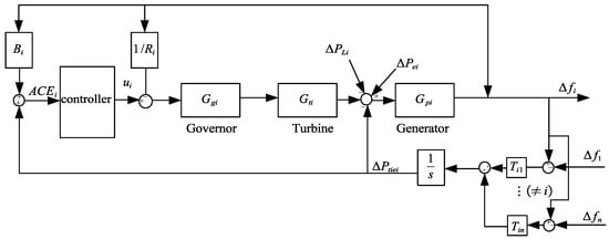
Figure 1.
Block diagram of control area .
In Figure 1, , and represent the transfer functions of the governor, turbine, and generator of area , respectively. For this system, it is simple to determine the relationship among the deviation of the frequency and the input of the control :
where is the load disturbance in this area; the output power deviation generated by renewable energy sources is denoted as . The tie-line exchanged power can be expressed as:
The Area Control Error (ACE) is a crucial parameter in the AGC system responsible for maintaining a balance between the real-time generation and demand. The AGC system continuously adjusts the generator’s power output to regulate the ACE and keep the system frequency within an acceptable range. Typically, ACE can be expressed as:
2.1. Two-Area Interconnected Power System with Solar Thermal Power Plant
Figure 2 shows the framework schematic for the two-area interconnected power system with solar thermal power plants [32], with its parameters and meanings listed in Table 2. As shown in the diagram, the power grid under study consists of two interconnected areas, each area of a STPP and a fuel unknit comprising of a single reheat turbine. The governor and the reheat turbine are both important components of the AGC system, with the governor primarily being used to control the velocity of the turbine power section and the non-reheat turbine being used to supply mechanical power to the generator [33]. We have utilized nonlinear links comprising of a governor dead band (GDB) of 0.06% (0.036 Hz) and a generation rate constraint (GRC) of 3%/min, with the intention of bringing the entire system closer to reality.
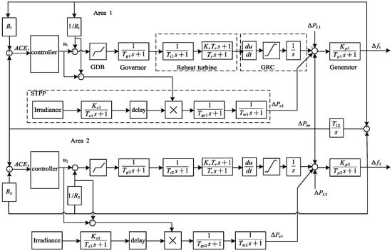
Figure 2.
Transfer function model of the two-area interconnected power system.
Table 2.
Symbolic representation of two-area interconnected power system with STPP.
A STPP is a type of power generation plant that converts solar energy into usable electricity. The process begins with a large field of mirrors, called heliostats, which track the sun and reflect its rays onto a receiver located at the top of a central tower. The receiver absorbs the heat from the concentrated sunlight, which is then used to heat a fluid, usually a synthetic oil, that flows through the receiver [34]. The heated fluid is then sent to a heat exchanger where it heats water to produce steam. The steam drives a turbine, which in turn generates electricity. Typically, is used to describe the receiver’s transfer function, where is time constant and denotes solar field gain. Due to the inherent response latency of the control system regarding variations in solar irradiance or tracking adjustments, the STPP also accounts for a nominal one-second delay.
The STPP’s output power may be determined through Figure 2 and is as follows:
and the frequency deviation is:
where , , .
Then, the is:
2.2. Five-Area Interconnected Power System with WTG-PV-Thermal-Hydro-Gas
The structure diagram of a five-area interconnected power system is shown in Figure 3. Area 1 is interconnected with Areas 2, 3, and 4, while Area 5 is interconnected with Areas 2, 3, and 4, and Area 5 is only interconnected with Area 1. Additionally, each of the five areas has a distinctive framework, including WTG, PV systems, thermal power generator, hydro turbines [18], and natural gas units [17]. The meaning and specific parameters of the researched model are detailed in Table 3.
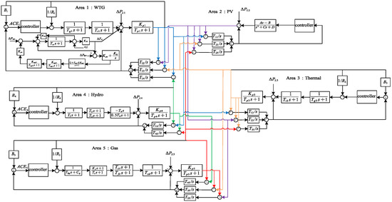
Figure 3.
Transfer function model of the five-area interconnected power system.
Table 3.
Symbolic representation of the five-area interconnected power system.
The calculation of the expression that describes the relationship between the controller input and the controller output can be derived in a similar way as shown in Equations (1)–(3), resulting in the following expressions:
However, it is worth noting that Area 2 does not have an ACE, and the input to the controller is . For Area 4, it can be seen from its transfer function that there are zeros in the right half-plane of the complex plane. Therefore, a compensator, such as the one proposed in reference [35], needs to be added.
From the above analysis, it is evident that in a mixed multi-area interconnected power system, such as the one mentioned above, means a single area can be subjected to both load disturbances (internal disturbances) and the influence of other areas (external disturbances). Additionally, there may be unmodeled dynamics and parameter perturbations, which can have an adverse effect on the entire system. Therefore, designing a controller that responds quickly and can overcome disturbances is of utmost importance.
3. Design of NFOADRC
The most frequently employed technique for load frequency control is called tie-line bias control (TBC), which employs ACE as the input signal to the controller, so that and can be simultaneously stabilized at 0. In LADRC, the LESO can observe disturbances even when the system model is unknown. This feature of LESO satisfies the requirements of LFC. Additionally, compared to classical integer-order PD controllers, FOPD controllers have better interference suppression and faster response times, making them more robust. As a result, this paper chooses to combine LADRC and FOPD to create a unique FOADRC, abbreviated as NFOADRC, for controlling the power system’s load frequency.
The power exchange between the tie lines can be overlooked throughout the design of the controller phase. Let , then the input–output relationship of the system is as follows:
where , , and denote the Laplace transform of , and , respectively, which represent the system’s input, output, and disturbance. Generally, and can be represented as follows:
Then, with a total order of , the system can be compactly abbreviated as follows:
where is the total disturbance.
Equation (12) can generally be simplified as
where is the compensator coefficient of the system.
In fact, when using NFOADRC to control each area of the interconnected power system separately, LESO needs to know the order of the system in each area to effectively estimate the disturbance of the system. Therefore, we also need to calculate the system order of each area in the interconnected power system, which will be provided in the subsequent simulation experiments.
In this paper, the structure of the NFOADRC designed is illustrated in Figure 4. The most crucial aspect of this controller is the LESO that estimates the total disturbance of the system, along with the FOPD controller that compensates for the disturbance . For an n-order system represented by Equation (16), the state equation can be obtained by setting , , …, , , then it can be obtained that the state equation is
and the LESO can be designed as follows:
where , , …, , are the estimates of , , …, , , and is the observation gain vector:
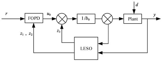
Figure 4.
Structure of the NFOADRC.
To facilitate practical applications, the pole placement method [36] is commonly used to configure the observer gain at the pole of , as shown in Equation (20).
The disturbance can then be eliminated using fractional-order control laws, as shown in Equations (21) and (22).
where is the output of the FOPD controller.
The FOPD controller’s transfer function is provided by:
where and are the proportional and differential gains, respectively, is the fractional order and .
It can be observed that the FOPD controller has parameters. To facilitate tuning, we can also use the pole-placement method to configure it at the pole of , as shown in Equation (23).
Therefore, tuning the parameters of NFOADRC can be transformed into tuning the parameters , and .
4. NFOADRC Parameter Tuning Based on IMPA
The pole-placement method can significantly reduce the number of parameters in NFOADRC; however, the parameter tuning issue still needs to be considered. This is because the parameters of the NFOADRC directly affect its control effect, which is still an indispensable part of controller design. MPA is a new natural-inspired algorithm proposed in recent years. The inspiration for this algorithm comes from the characteristics of predators and prey in nature. It uses an adaptive step-size strategy, which can continuously adjust the step size in the search process, thus speeding up the search process and improving the convergence speed. However, it also has shortcomings, such as uneven initial position selection and easy entrapment in local optima during the iterative process. Therefore, this paper needs to improve MPA from the following aspects and apply it to the parameter tuning of NFOADRC.
4.1. Design of Improved Marine Predator Algorithm
- (1)
- Chaotic opposite-based learning strategy
To address the issue of uneven initial position distribution, a new strategy called “Chaotic Opposition-based Learning” (COBL) is proposed. COBL combines the Tent map chaos [37] with the opposition-based learning strategy [38], forming a new Tent and Opposition-based Learning (TOBL) mechanism. The mathematical model of TOBL is as follows:
where represents the -th component of the -th prey’s opposite position. and are the upper and lower bounds of the objective function, respectively. represents the chaotic number generated by using the Tent map in the -th iteration.
The TOBL strategy can be thought of as a dynamic compression of the initial population distribution range, using the uniform variation of Tent, with the sum of the upper and lower bounds of the objective function as the center. This compression is carried out in such a way as to achieve uniformity in the population distribution as much as possible.
- (2)
- Gaussian distribution
After updating the position of the prey in the fundamental MPA, it is important to find and update the location of the top predator and carry out one marine memory storage. Next, the influence of FADs is considered to further update the prey’s position. In order to ensure the effectiveness of this memory storage, a Gaussian distribution operator is introduced. Before simulating the influence of FADs, the position of the prey is mutated using the Gaussian distribution operator. If the mutated position is better, it replaces the original position. The mathematical model is as follows:
- (3)
- Grouping dimension learning strategy
Some prey position dimensions have potentially reached their optimum position during an algorithm iteration in the past. However, the fitness of these prey situations could deteriorate as a result of the effect of specific individual dimensions. A grouping dimension learning approach is suggested as a solution to this problem. After the impact of FADs, the prey is sorted according to their fitness and then divided into two groups: the elite group, which consists of individuals with high fitness, and the learning group, which consists of individuals with low fitness [39].
Due to the fact that each dimension of the elite group has its own strengths and weaknesses, the average value of the dimensions of the elite group’s position is taken. Each prey in the learning group leans towards the average dimensions of the elite group. This strategy calculates the difference between each dimension of each prey in the learning group and the average dimension of the elite group. Then, it follows the principle of prioritizing those with larger absolute differences, and selects the top dimensions with the largest absolute differences for crossover one by one. If the fitness of the prey is improved after the crossover, the corresponding dimensions are crossed; otherwise, they are not crossed. The mathematical model of this strategy is as follows:
where is the position of the -th prey in the learning group, represents the position of the -th prey after crossing with the -th dimension of the average dimension value of the elite group, denotes the absolute difference between the -th dimension of the -th prey in the learning group and the -th dimension of the average dimension value of the elite group, and represents the -th dimension of the average value of the elite group.
The learning group dimension crossover strategy refers to the grouping of individuals based on grouping information during crossover operations, rather than performing a crossover on each dimension like in normal genetic algorithms. This approach ensures that the individuals within each group have more similar fitness, which can maintain population diversity and improve search efficiency. It is important to note that during learning group dimension crossover, the crossover operation between individuals is not performed independently, however, it takes into account the similarity within the group. Therefore, the algorithm adopts a similarity-based crossover probability adjustment strategy, where individuals with a higher similarity have a lower crossover probability, and individuals with a lower similarity have a higher crossover probability, to balance population diversity and convergence speed.
In the elite group dimension crossover strategy, the elite group is considered a subset of individuals with excellent fitness. Since the elite group is relatively close to the global optimum, it is not suitable for perturbation mutation on all dimensions, as this may cause the elite individuals to linger around the optimal solution and affect convergence accuracy. Instead, the prey of the elite group learns from each other by exchanging their advantages and improving their deficiencies while retaining their own advantageous dimensions. The crossover principle of this strategy is the same as that of the learning group prey crossover strategy, except that the crossover pair is replaced by the neighboring prey of the current prey, and the elite group exchanges the top neighboring corresponding dimensions with the greatest absolute difference. This strategy only moves the individuals towards the direction of the dimension being crossed, which preserves other advantageous dimensions. Compared with the mutation of the entire individual, this strategy has stronger selection superiority, which can effectively enhance the algorithm’s dimension depth mining performance and improve convergence accuracy.
4.2. IMPA Optimized NFOADRC
In multi-area interconnected power systems, the increase in frequency deviation is not only caused by factors such as the parallel connection of renewable energy grids and external disturbances, but also by inappropriate controller parameter settings. Therefore, in order to achieve a better load frequency control and improve the power system quality, this paper chooses IMPA to adjust the parameters of NFOADRC.
For the designed NFOADRC in this paper, the only parameters that need to be optimized are and , while has little effect on the system’s stability, and is therefore fixed [40]. The selection of parameter needs to be based on the actual situation and experience of the system because intelligent algorithms can usually optimize the performance of the system, however, they cannot guarantee its stability. If intelligent algorithms are used to tune , it may lead to an unstable system. Therefore, this paper adopts the method in reference to [41] to select . The implementation process of IMPA is as follows:
- Initialize the position of the prey using chaotic opposition-based initialization and set related parameters such as population size, maximum number of iterations, FADs, etc.
- Compute the fitness value of each prey, compare and replace the fitness values, and construct the top predator matrix consisting of the best prey, and perform ocean memory storage.
- Update the position and step size of the prey.
- Perform position disturbance update using the Gaussian mutation operator of Equation (25) and retain the best position.
- Recalculate the fitness value of each prey, compare and replace the fitness values, construct the top predator matrix consisting of the best prey, and store the memory of the ocean.
- Consider the influence of FADs and vortices and further update the position while retaining the best position.
- Divide the updated population into learning groups and elite groups with equal fitness based on Equations (26) and (27), and perform dimensional crossover, crossing the corresponding dimension if the fitness improves and vice versa.
- Check whether the iteration condition is satisfied. If yes, terminate the algorithm, otherwise return to step 2.
When optimizing the parameters of the IMPA controller, the Integral Time Absolute Error (ITAE) is selected as the fitness function, as . The principle diagram of parameter optimization based on IMPA is shown in Figure 5.
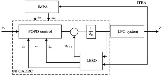
Figure 5.
IMPA-based NFOADRC control structure diagram.
5. Simulation Results and Discussions
In this section, we first select nine test functions to compare and analyze the optimization performance of the proposed IMPA algorithm with MPA [30], WOA [28], and CWOA [29]. Then, based on the two models introduced in Section 2, we implement the IMPA-NFOADRC method and further analyze the simulation results.
5.1. Benchmark Function Tests
The test functions include three multidimensional single-peaked functions, F1–F3, three multidimensional multi-peaked functions, F4–F6, and three fixed-dimension multi-peaked functions, F7–F9 [42]. The specific function information is shown in Table 4. All algorithms were set to 200 iterations with a population of 40. The multidimensional test function has a dimension of 50, while the fixed-dimension functions F7–F8 have 4 dimensions, and F8 has 3 dimensions. Each algorithm was independently run 30 times to calculate the best fitness value, the average best fitness value, and the standard deviation of the best fitness value among the 30 runs.
Table 4.
Test function.
Figure 6 depicts the convergence curves of the four algorithms in 30-dimensional space for three unimodal test functions, three multimodal test functions, and three fixed-dimensional test functions.
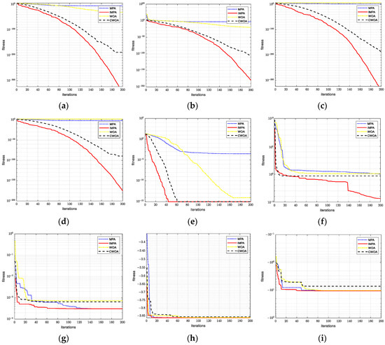
Figure 6.
Convergence curve of partial function: (a) F1 iterative curve; (b) F2 iterative curve; (c) F3 iterative curve; (d) F4 iterative curve; (e) F5 iterative curve; (f) F6 iterative curve; (g) F7 iterative curve; (h) F8 iterative curve; (i) F9 iterative curve.
Based on the data in Table 5, it is evident that IMPA demonstrates a remarkable performance in optimizing unimodal functions. It achieves optimal solutions and average values closest to zero, with a standard deviation of zero. This highlights the clear advantage of the proposed IMPA algorithm over MPA, WOA, and CWOA in the optimization of unimodal functions. Moreover, IMPA exhibits excellent performance in handling multimodal functions, as its optimal solutions closely approximate the theoretical optimal values of the benchmark functions. This consistency is not coincidental, as the average values of IMPA are closer to zero compared to the other three algorithms, indicating that each optimization result is closer to the theoretical optimum. Furthermore, even in the presence of multiple local optima, IMPA effectively avoids becoming trapped in such suboptimal solutions. For the three fixed-dimensional multimodal functions, the theoretical optimal solutions are 0.0003, −3.32237, and −10.5363, respectively. From Table 5, it can be observed that only MPA and IMPA achieve optimal values of 0.0003075, −3.322, and −10.536, respectively, which are closest to the theoretical optima. Additionally, the smaller standard deviation of the multiple optimization results further confirms the superior optimization capabilities of IMPA compared to the other three algorithms. This superiority of IMPA is also reflected in Figure 6, where the red curve represents the optimization curve based on IMPA. It is evident that IMPA not only converges faster than other algorithms but also approaches the theoretical optimum more closely. Hence, the proposed IMPA algorithm exhibits significant advantages over WPA, WOA, and CWOA in the field of function optimization.
Table 5.
Test data of function.
5.2. Control of Two-Area Interconnected Power System with Solar Thermal Power Plant
This article’s first model is a two-area interconnected power system, as shown in Figure 2. These two areas have the same structure and parameters and are controlled by controllers designed with the same parameters. Below, we will illustrate the design of the controller for Area 1, as an example. Firstly, the design of LESO in NFOADRC requires knowledge of the order of the system, which can be determined using the following equations.
where . Then, we can get the system order is 3.
Suppose that step load perturbation (SLP), p.u. is added in Area I at s. The population size for IMPA, MPA, CWOA, and WOA are all set to 50, and the maximum number of iterations is set to 30. Additionally, the fitness function chosen for parameter optimization in all cases was the integrated time and absolute error (ITAE) as .
Then, to compare the performance indicators of the controllers, NFOADRC, PID [20], FOPID [43], and LADRC [18] were applied to the same interconnected power system. In the NFOADRC, is set to 0.05 and is set to 20. The ranges of values for and optimized using IMPA are determined as: , and the optimized results are as follows: . To make a fair comparison, the value of in the LADRC is also set to 20, and the range of values for and are set as follows: . The optimization results using MPA are and ; The parameter ranges for the three PID controller parameters are set as follows: . The optimization result obtained by CWOA are: . The integral order and derivative order of the FOPID controller, along with its three parameters, are set to the following ranges: . And the optimization result obtained by WOA are: .
The response curves obtained by applying the above controllers to the two-area interconnected power system are shown in Figure 7. Table 6 illustrates the various specifications of the system performance, such as overshoot (), undershoot (), and settling time (). Additionally, the settling time is defined as the shortest time required for the output to reach and stabilize within .
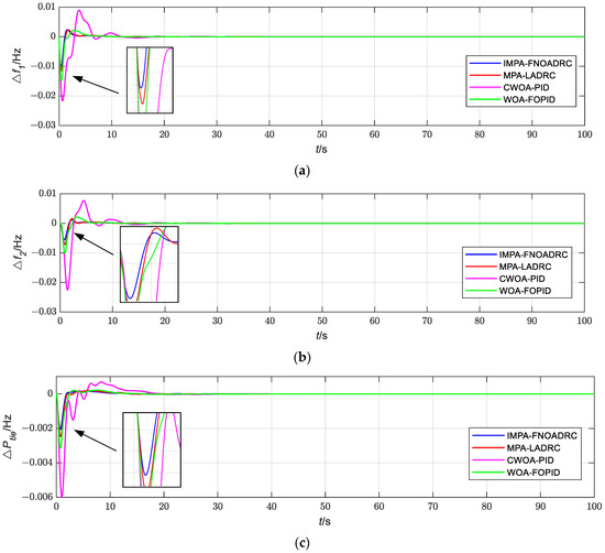
Figure 7.
Dynamic power grid responses of the two-area interconnected power system when (a) Frequency deviation of Area 1. (b) Frequency deviation of Area 2. (c) Tie-line exchanged power.
Table 6.
Comparison of the transient response specifications of two-area power systems.
From Figure 7, it can be observed that in the steady state, the frequency deviation and tie-line exchanged power of each area stabilize at 0 under the control, indicating a similar steady-state performance of the controllers. From Table 6, it is evident that in Area 1, IMPA-NFOADRC exhibits a decrease in undershoot compared to CWOA-PID by 0.0102, which corresponds to a reduction of 52.99%. Compared to WOA-FOPID, it decreases by 0.0047, equivalent to a decrease of 31.54%. In comparison to MPA-LADRC, it decreases by 0.0115, which corresponds to an 11.30% reduction. Overall, IMPA-NFOADRC demonstrates a smaller undershoot in frequency deviation in Area 1, indicating a smaller undershoot. Regarding overshoot, IMPA-NFOADRC reduces it by 73.33% compared to CWOA-PID, which decreases it by 7.69% compared to WOA-FOPID, and matches MPA-LADRC’s overshoot. In terms of settling time, IMPA-NFOADRC clearly exhibits a shorter settling time.
Similarly, in Area 2, it can be analyzed that IMPA-NFOADRC exhibits a decrease in undershoot of 21.12% compared to MPA-LADRC, a reduction in overshoot of 31.25%, and a shortening of settling time by 4.22 s. In terms of tie-line exchanged power, IMPA-NFOADRC shows a decrease in undershoot of 19.05% compared to MPA-LADRC, a reduction in overshoot of 50%, and a reduction in settling time by 1.07 s.
From the simulation results, it can be observed that the proposed method in this study outperforms the other three methods in terms of undershoot, overshoot, and settling time in the control of the two-area interconnected power system. This superiority can be attributed to the introduction of fractional-order differentiation in IMPA-NFOADRC, which expands the frequency response characteristics of the controller, enabling better suppression of fast oscillations and noise interference in the system. When frequency deviation occurs or an area control error increases, NFOADRC can adjust more quickly and accurately, maintaining the system in a stable operating state, resulting in reduced undershoot, overshoot, and shorter settling time.
5.3. Control of Five-Area Interconnected Power System with WTG, PV, Gas and Hydro Turbine
This article’s second model is a five-area interconnected power system, as shown in Figure 3. Each area has its own unique structure and parameters, including wind turbines, photovoltaic power generation, thermal turbines, hydro turbines, and natural gas units. Therefore, the parameters of designed controllers for each area are also distinct. For the first area, the transfer function is provided as follows:
Therefore, the order of the system in the first area can be determined as 3. Similarly, we can obtain the system orders of the remaining four areas as 2, 3, 3, and 3, respectively.
To validate the control performance of the NFOADRC optimized based on IMPA in a five-area interconnected grid under step-load perturbation (SLP) and renewable energy influence, two types of disturbances are assumed:
- (1)
- At s, the SLP with p.u. was added to Areas 1, 3, and 5. At s, the SLP with p.u. was added to Areas 2 and 4.
- (2)
- At s and s, the SLP of p.u. will be applied to all five areas.
Furthermore, a LADRC controller based on MPA optimization is employed to control a five-area interconnected power system under the same conditions, and their system response results are compared.
Then, under these two types of disturbances, the system response results of the five-area interconnected power grid will be compared when controlled using the NFOADRC optimized by IMPA and the LADRC optimized by MPA, both under the same conditions. The values of for the five areas are 50, 40, 40, 8000, and 8000, respectively. is equal to 0.2. The parameters’ domain for five areas have been set as follows: , , , . The optimization results of the controller parameters under the two disturbances are shown in Table 7, and the corresponding power system responses are depicted in Figure 8 and Figure 9.
Table 7.
Optimization results of controller parameter.
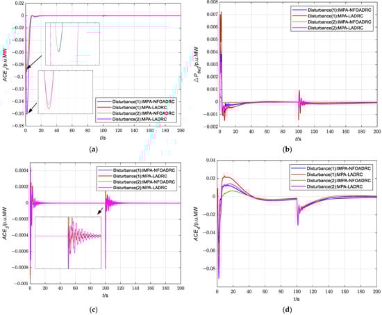
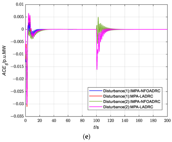
Figure 8.
Controller input: (a) ; (b) ; (c) ; (d) ; (e) .
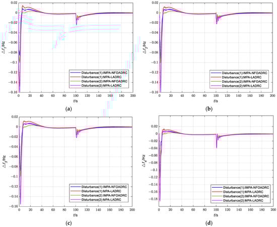
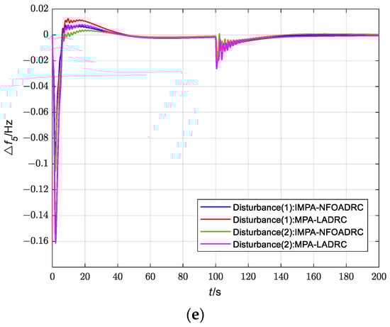
Figure 9.
Frequency deviation of the five-area interconnected power system: (a)Frequency deviation of Area 1; (b) Frequency deviation of Area 2; (c) Frequency deviation of Area 3; (d) Frequency deviation of Area 4; (e) Frequency deviation of Area 5.
Figure 8 illustrates the comparison of area control errors in the five-area interconnected power system under two different disturbances. Table 8 and Table 9 present the undershoot, overshoot, and percentage improvement of IMPA-NFOADRC compared to MPA-LADRC for each area under disturbance (1) and disturbance (2), respectively. From Figure 8, it can be observed that both IMPA-NFOADRC and MPA-LADRC stabilize the entire system under both disturbances, however IMPA-NFOADRC exhibits smaller errors. Specifically, Table 8 and Table 9 show that IMPA-NFOADRC reduces undershoot and overshoot in regional control errors by approximately 20% to 40%, compared to MPA-LADRC.
Table 8.
Comparison of area control errors in a five-area power system under disturbance (1).
Table 9.
Comparison of area control errors in a five-area power system under disturbance (2).
Figure 9 displays the comparison of frequency deviation under two different disturbances, while Table 10 and Table 11 represent the undershoot, overshoot, and percentage improvement for each corresponding metric. From Figure 9, it is evident that IM-PA-NFOADRC achieves a smaller frequency deviation compared to MPA-LADRC, regard-less of the disturbance type. This observation is further supported by Table 10 and Table 11, which show that IMPA-NFOADRC reduces undershoot and overshoot in frequency deviation by approximately 35% to 55%, compared to MPA-LADRC.
Table 10.
Comparison of frequency deviation in a five-area power system under disturbance (1).
Table 11.
Comparison of frequency deviation in a five-area power system under disturbance (2).
In conclusion, the proposed IMPA-optimized NFOADRC in this paper exhibits smaller frequency deviation and area control error compared to MPA-LADRC. This superiority can be attributed to several factors. Firstly, NFOADRC possesses the characteristics of a fractional-order controller, which enables it to have better frequency response properties and effectively overcome system instability, thereby reducing frequency deviation and area control error. Secondly, the improvements in the initial population distribution and escaping local optima of IMPA result in a more flexible parameter adjustment capability compared to MPA. This enhanced adaptability allows IMPA to better cope with system variations and uncertainties.
6. Conclusions
In this paper, a novel fractional-order adaptive controller (NFOADRC) based on an improved marine predator algorithm (IMPA) optimization is proposed for load frequency control (LFC) in automatic generation control systems containing renewable energy sources. Firstly, the performance of the IMPA was enhanced by using chaotic opposition-based initialization, Gaussian distribution mutation operator, and group dimension learning, which improves its optimization performance as demonstrated by testing on nine benchmark functions. Next, taking advantage of the strong disturbance suppression capability and fast response time of the FOPD controller, the LADRC was improved to form the NFOADRC. The proposed algorithm was employed to tune its parameters. The simulation results on two-area and five-area interconnected power systems demonstrated that the proposed method outperforms LADRC, PID, and FOPID in terms of performance metrics, such as overshoot, undershoot, and settling time. Moreover, the proposed method effectively overcomes the effects of SLP and renewable energy sources, making it an efficient approach for LFC.
As the application of fractional-order control methods in practical experiments is still limited, future research will focus on applying the method proposed in this paper to real-world scenarios. Additionally, the parameter ranges optimized by IMPA in this study were manually selected, and the precise and feasible ranges of controller parameters also need to be analyzed and determined in the next step.
Author Contributions
Conceptualization, W.H. and Y.Z. (Yuemin Zheng); methodology, W.H. and Y.Z. (Yujuan Zhou); software, W.H. and Y.Z. (Yuemin Zheng); validation, Q.S., Y.Z. (Yujuan Zhou) and J.T.; formal analysis, W.H. and Y.Z. (Yuemin Zheng); investigation, W.H.; resources, Y.Z. (Yuemin Zheng); data curation, W.H.; writing—original draft preparation, W.H.; writing—review and editing, J.T., J.W. and Y.Z. (Yuemin Zheng); supervision, J.T. and J.W.; funding acquisition, J.W. All authors have read and agreed to the published version of the manuscript.
Funding
This research was funded by the National Natural Science Foundation of China, Grant/Award Number: 61963006, the National Science Foundation of Guangxi Province of China, Grant/Award Number: 2018GXNSFAA050029 and 2018GXNSFAA294085, the Major Science and Technology Projects in Guangxi, Grant/Award Number: Guike AA22068064, and the Industry-University-Research Innovation Fund for Chinese Universities, Grant/Award Number: 2021ZYA08002.
Institutional Review Board Statement
Not applicable.
Informed Consent Statement
Not applicable.
Data Availability Statement
Data sharing not applicable.
Conflicts of Interest
The authors declare no conflict of interest.
Appendix A
Table A1.
Abbreviation Key.
Table A1.
Abbreviation Key.
| Abbreviations | Full Forms |
|---|---|
| LFC | Load frequency control |
| AGC | Automated generation control |
| ACE | Area control error |
| GDB | Governor dead band |
| GRC | Generation rate constraint |
| TBC | Tie-line bias control |
| STPP | Solar thermal power plant |
| WTG | Wind turbine generator |
| PV | Photovoltaic |
| SLP | Step load perturbation |
| IMPA | Improved marine predator algorithm |
| WOA | Whale optimization algorithm |
| CWOA | Chaotic whale optimization algorithm |
| MPA | Marine predators algorithm |
| COBL | Chaotic opposition-based learning |
| TOBL | Tent and opposition-based learning |
| FAD | Fish aggregating devices |
| ITAE | Integrated time and absolute error |
| NFOADRC | Novel fractional order active disturbance rejection controller |
| PID | Proportional-integral-derivative |
| MPC | Model predictive controller |
| SMC | Sliding mode controller |
| LADRC | Linear active disturbance rejection controller |
| LESO | Linear extended state observer |
| IOPD | Integer-order PD |
| FOPD | Fractional-order PD |
References
- Abazari, A.; Soleymani, M.M.; Babaei, M.; Ghafouri, M.; Monsef, H.; Beheshti, M.T.H. High penetrated renewable energy sources-based AOMPC for microgrid’s frequency regulation during weather changes, time-varying parameters and generationunit collapse. IET Gener. Transm. Distrib. 2020, 14, 5164–5182. [Google Scholar] [CrossRef]
- Khan, I.A.; Mokhlis, H.; Mansor, N.N.; Illias, H.A.; Awalin, L.J.; Wang, L. New trends and future directions in load frequency control and flexible power system: A comprehensive review. Alex. Eng. J. 2023, 71, 263–308. [Google Scholar] [CrossRef]
- Jalali, N.; Razmi, H.; Doagou-Mojarrad, H. Optimized fuzzy self-tuning PID controller design based on Tribe-DE optimization algorithm and rule weight adjustment method for load frequency control of interconnected multi-area power systems. Appl. Soft Comput. 2020, 93, 106424. [Google Scholar] [CrossRef]
- Zheng, Y.; Zhou, J.; Xu, Y.; Zhang, Y.; Qian, Z. A distributed model predictive control based load frequency control scheme for multi-area interconnected power system using discrete-time Laguerre functions. ISA Trans. 2017, 68, 127–140. [Google Scholar] [CrossRef] [PubMed]
- Kumar, R.; Sikander, A. A novel load frequency control of multi area non-reheated thermal power plant using fuzzy PID cascade controller. Sādhanā 2023, 48, 25. [Google Scholar] [CrossRef]
- Zhong, Q.; Yang, J.; Shi, K.; Zhong, S.; Li, Z.; Sotelo, M.A. Event-triggered H∞ load frequency control for multi-area nonlinear power systems based on non-fragile proportional integral control strategy. IEEE Trans. Intell. Transp. Syst. 2021, 23, 12191–12201. [Google Scholar] [CrossRef]
- Khamies, M.; Magdy, G.; Ebeed, M.; Kamel, S. A robust PID controller based on linear quadratic gaussian approach for improving frequency stability of power systems considering renewables. ISA Trans. 2021, 117, 118–138. [Google Scholar] [CrossRef]
- Sun, J.; Chen, M.; Kong, L.; Hu, Z.; Veerasamy, V. Regional load frequency control of BP-PI wind power generation based on particle swarm optimization. Energies 2023, 16, 2015. [Google Scholar] [CrossRef]
- Gulzar, M.M.; Iqbal, M.; Shahzad, S.; Muqeet, H.A.; Shahzad, M.; Hissaom, M.M. Load frequency control (LFC) strategies in renewable energy-based hybrid power systems: A review. Energies 2022, 15, 3488. [Google Scholar] [CrossRef]
- Ali, H.H.; Fathy, A.; Kassem, A.M. Optimal model predictive control for LFC of multi-interconnected plants comprising renewable energy sources based on recent sooty terns approach. Sustain. Energy Technol. Assess. 2020, 42, 100844. [Google Scholar] [CrossRef]
- Yousri, D.; Babu, T.S.; Fathy, A. Recent methodology based Harris Hawks optimizer for designing load frequency control incorporated in multi-interconnected renewable energy plants. Sustain. Energy Grids Netw. 2020, 22, 100352. [Google Scholar] [CrossRef]
- Mani, P.; Joo, Y.H. Fuzzy logic-based integral sliding mode control of multi-area power systems integrated with wind farms. Inf. Sci. 2021, 545, 153–169. [Google Scholar] [CrossRef]
- Oshnoei, S.; Oshnoei, A.; Mosallanejad, A.; Hahjoo, F. Novel load frequency control scheme for an interconnected two-area power system including wind turbine generation and redox flow battery. Int. J. Electr. Power Energy Syst. 2021, 130, 107033. [Google Scholar] [CrossRef]
- Sobhy, M.A.; Abdelaziz, A.Y.; Hasanien, H.M.; Ezzat, M. Marine predators algorithm for load frequency control of modern interconnected power systems including renewable energy sources and energy storage units. Ain Shams Eng. J. 2021, 12, 3843–3857. [Google Scholar] [CrossRef]
- Vedik, B.; Kumar, R.; Deshmukh, R.; Verma, S.; Shiva, C.K. Renewable energy-based load frequency stabilization of interconnected power systems using quasi-oppositional dragonfly algorithm. J. Control Autom. Electr. Syst. 2021, 32, 227–243. [Google Scholar] [CrossRef]
- Khadanga, R.K.; Kumar, A.; Panda, S. A modified grey wolf optimization with cuckoo search algorithm for load frequency controller design of hybrid power system. Appl. Soft Comput. 2022, 124, 109011. [Google Scholar] [CrossRef]
- Elkasem, A.H.; Khamies, M.; Hassan, M.H.; Agwa, A.M.; Kamel, S. Optimal design of TD-TI controller for LFC considering renewables penetration by an improved chaos game optimizer. Fractal Fract. 2022, 6, 220. [Google Scholar] [CrossRef]
- Zheng, Y.; Tao, J.; Sun, Q.; Sun, H.; Chen, Z.; Sun, M. Deep reinforcement learning based active disturbance rejection load frequency control of multi-area interconnected power systems with renewable energy. J. Frankl. Inst. 2022; in press. [Google Scholar] [CrossRef]
- Halmous, A.; Oubbati, Y.; Lahdeb, M.; Arif, S. Design a new cascade controller PD-P-PID optimized by marine predators algorithm for load frequency control. Soft Comput. 2023, 27, 9551–9564. [Google Scholar] [CrossRef]
- Ali, T.; Malik, S.A.; Daraz, A.; Adeel, M.; Aslam, S.; Herodotou, H. Load frequency control and automatic voltage regulation in four-area interconnected power systems using a gradient-based optimizer. Energies 2023, 16, 2086. [Google Scholar] [CrossRef]
- Chen, D.; Li, S.; Wu, Q. A novel supertwisting zeroing neural network with application to mobile robot manipulators. IEEE Trans. Neural Netw. Learn. Syst. 2020, 32, 1776–1787. [Google Scholar] [CrossRef] [PubMed]
- Lu, H.; Jin, L.; Luo, X.; Liao, B.; Gup, D.; Xiao, L. RNN for solving perturbed time-varying underdetermined linear system with double bound limits on residual errors and state variables. IEEE Trans. Ind. Inform. 2019, 15, 5931–5942. [Google Scholar] [CrossRef]
- Khooban, M.H.; Niknam, T.; Blaabjerg, F.; Davari, P.; Dragicevic, T. A robust adaptive load frequency control for micro-grids. ISA Trans. 2016, 65, 220–229. [Google Scholar] [CrossRef] [PubMed]
- Gao, Z. On the centrality of disturbance rejection in automatic control. ISA Trans. 2014, 53, 850–857. [Google Scholar] [CrossRef]
- Wang, Y.; Tan, W.; Cui, W.; Han, W.; Guo, Q. Linear active disturbance rejection control for oscillatory systems with large time-delays. J. Frankl. Inst. 2021, 358, 6240–6260. [Google Scholar] [CrossRef]
- Safiullah; Hote, V.Y. Reduced Order Based Active Disturbance Rejection Controller Design with Applications. IETE Tech. Rev. 2023, 1–18. [Google Scholar] [CrossRef]
- Chen, P.; Luo, Y. A two-degree-of-freedom controller design satisfying separation principle with fractional-order PD and generalized ESO. IEEE/ASME Trans. Mechatron. 2021, 27, 137–148. [Google Scholar] [CrossRef]
- Mirjalili, S.; Lewis, A. The whale optimization algorithm. Adv. Eng. Softw. 2016, 95, 51–67. [Google Scholar] [CrossRef]
- Kaur, G.; Arora, S. Chaotic whale optimization algorithm. J. Comput. Des. Eng. 2018, 5, 275–284. [Google Scholar] [CrossRef]
- Faramarzi, A.; Heidarinejad, M.; Mirjalili, S.; Gandomi, A.H. Marine Predators Algorithm: A nature-inspired metaheuristic. Expert Syst. Appl. 2020, 152, 113377. [Google Scholar] [CrossRef]
- Wang, S.; Zhu, H.; Zhang, S. Two-stage grid-connected frequency regulation control strategy based on photovoltaic power prediction. Sustainability 2023, 15, 8929. [Google Scholar] [CrossRef]
- Singh, A.; Sharma, V. Salp swarm algorithm-based model predictive controller for frequency regulation of solar integrated power system. Neural Comput. Appl. 2019, 31, 8859–8870. [Google Scholar] [CrossRef]
- Zheng, Y.; Huang, Z.; Tao, J.; Sun, H.; Sun, Q.; Sun, M.; Chen, Z. A novel chaotic fractional-order beetle swarm optimization algorithm and its application for load-frequency active disturbance rejection control. IEEE Trans. Circuits Syst. II Express Briefs 2021, 69, 1267–1271. [Google Scholar] [CrossRef]
- Feleke, S.; Satish, R.; Pydi, B.; Anteneh, D.; Abdelaziz, A.Y.; EI-Shahat, A. Damping of Frequency and Power System Oscillations with DFIG Wind Turbine and DE Optimization. Sustainability 2023, 15, 4751. [Google Scholar] [CrossRef]
- Tan, W. Unified tuning of PID load frequency controller for power systems via IMC. IEEE Trans. Power Syst. 2009, 25, 341–350. [Google Scholar] [CrossRef]
- Gao, Z. Active disturbance rejection control: A paradigm shift in feedback control system design. In Proceedings of the 2006 American Control Conference (IEEE), Minneapolis, MN, USA, 14–16 June 2006. [Google Scholar]
- Valle, J.; Machicao, J.; Bruno, O.M. Chaotical PRNG based on composition of logistic and tent maps using deep-zoom. Chaos Solitons Fractals 2022, 161, 112296. [Google Scholar] [CrossRef]
- Yuan, Y.; Mu, X.; Shao, X.; Ren, J.; Zhao, Y.; Wang, Z. Optimization of an auto drum fashioned brake using the elite opposition-based learning and chaotic k-best gravitational search strategy based grey wolf optimizer algorithm. Appl. Soft Comput. 2022, 123, 108947. [Google Scholar] [CrossRef]
- Guo, J.; Wang, Q.; Wang, X. Moth Flame Optimization based on learning strategy and neighborhood search. Comput. Eng. Appl. 2021, 57, 170–179. [Google Scholar]
- Xue, W.; Huang, Y. Performance analysis of active disturbance rejection tracking control for a class of uncertain LTI systems. ISA Trans. 2015, 58, 133–154. [Google Scholar] [CrossRef]
- Chen, P.; Luo, Y.; Zheng, W.; Gao, Z.; Chen, Y. Fractional order active disturbance rejection control with the idea of cascaded fractional order integrator equivalence. ISA Trans. 2021, 114, 359–369. [Google Scholar] [CrossRef]
- Zhong, K.; Luo, Q.; Zhou, Y.; Jiang, M. TLMPA: Teaching-learning-based Marine Predators algorithm. Aims Math. 2021, 6, 1395–1442. [Google Scholar] [CrossRef]
- Zaid, S.A.; Bakeer, A.; Magdy, G.; Albalawi, H.; Kassem, A.M.; EI-Shimy, M.E.; AbdelMeguid, H.; Manqarah, B. A new intelligent fractional-order load frequency control for interconnected modern power systems with virtual inertia control. Fractal Fract. 2023, 7, 62. [Google Scholar] [CrossRef]
Disclaimer/Publisher’s Note: The statements, opinions and data contained in all publications are solely those of the individual author(s) and contributor(s) and not of MDPI and/or the editor(s). MDPI and/or the editor(s) disclaim responsibility for any injury to people or property resulting from any ideas, methods, instructions or products referred to in the content. |
© 2023 by the authors. Licensee MDPI, Basel, Switzerland. This article is an open access article distributed under the terms and conditions of the Creative Commons Attribution (CC BY) license (https://creativecommons.org/licenses/by/4.0/).