Abstract
In order to mitigate the environmental pollution caused by sea freight, we focused on optimizing carbon emissions in container terminal operations. This paper establishes a mixed integer programming (MIP) model for a continuous berth allocation problem (CBAP) considering the tide time window. We aimed to minimize the total carbon emissions caused by the waiting time, consumption time and deviation to berth preference. In order to overcome the influence of an uncertain arrival time, the proposed MIP model was extended to mixed integer robust programming (MIRP) models, which applied a two-stage robust optimization (TSRO) approach to the optimal solution. We introduced an uncertainty set and scenarios to describe the uncertain arrival time. Due to the complexity of the resulting models, we proposed three particle swarm optimization (PSO) algorithms and made two novelties. The numerical experiment revealed that the robust models yielded a smaller variation in the objective function values, and the improved algorithms demonstrated a shorter solution time in solving the optimization problem. The results show the robustness of the constructed models and the efficiency of the proposed algorithms.
1. Introduction
Sustainable development has received widespread attention from various industries [1,2,3]. With the increase in the throughput of container terminals worldwide, maritime transport for trade and development has become increasingly important [4]. However, with the progress of human society and industrial manufacturing, the climate problem has become more and more serious. In 2021, according to the statistics of the International Energy Agency (IEA) on CO2 emissions in various fields in the world, the total carbon emissions of the transportation industry ranked second, accounting for less than 11% of the total [5]. These detailed data showed that land transportation accounted for 20%, while sea freight accounted for only 3%. However, according to the estimates of the United Nations Conference on Trade and Development (UNCTAD), the proportion of carbon dioxide produced by maritime transport activities in the total global carbon emissions may rise to 6% in 2022, and if no measures are taken by 2050, this figure may become 18% [6]. In addition, the environmental protection requirements of the shipping industry are set to gradually become stricter in the future. Therefore, realizing low-carbon and sustainable development is a future trend for the international shipping industry. To realize an economic and environmental co-development port, constructing a green container terminal could be a future direction of development [7].
In the link of terminal operation activities, berth planning and allocation are the first steps of a terminal operation. Efficient berth decision-making can help terminal operators reduce the time of container transshipment and yard transportation, thereby improving the traffic congestion at berths and yards, reducing emissions from terminal operations, and improving terminal service quality and environmental benefits. Therefore, Berth allocation has important practical significance, and this issue has always been a research hotspot of scholars. However, only some researchers have considered the effect of tide time conditions on vessel entry and departure in CBAP. In order to make this study more relevant to the actual situation, the deterministic MIP model was structured according to the current conditions of the continuous berth operation and took the influence of the tide time window on vessels in-wharf and out-wharf into account. This paper constructed a MIP model of CBAP to allocate the berth position, berthing time, and departure time for arrival vessels and to minimize the total emissions during the vessel berthing process.
Most of the early literature studied the berth allocation problem (BAP) in a deterministic environment, assuming that all parameters were known and invariable. However, as a highly complex and dynamic system, berth allocation in container terminals is particularly vulnerable to uncertain events [8,9]. The quality of berth allocation decisions can be significantly affected by frequent uncertain factors and unpredictable events. In addition, the berth plan is the basis of various operation planning in the terminal, and any adjustment to it could cause a series of changes to all subsequent operations. Therefore, it is essential to consider the impact of uncertainty in relevant decision-making.
In recent years, the related field of BAP under an uncertain environment has attracted the attention of many scholars and achieved specific results. Regarding the uncertainty research on issues relating to berth allocation, the modeling methods of uncertain BAP mainly focused on robust optimization (RO) [10], stochastic programming (SP) [11], fuzzy programming (FP) [12], etc. Among these, the RO method made up for the shortcomings of traditional optimization methods and had certain advantages. Although RO is gradually maturing with a high research value and practical application, these applications must be extended significantly in BAP. The most existing robust berth allocation problem (RBAP) in the research included uncertain optimization methods primarily focused on scenario-based stochastic programming and almost robust models, with few studies applying two-stage robust optimization (TSRO) methods. Moreover, for uncertain scenarios, a few studies were considered using machine learning techniques on historical data to handle multiple scenarios, aiming to estimate more accurate uncertain factors or construct uncertainty sets. In addition, almost all RBAP researchers have classified uncertain scenarios into multiple uncertainty sets, while the concept of the uncertainty set in robust classical theory still needs to be addressed. To bring the study closer to the real world, in this paper, the two-stage RO theory was applied to CBAP for uncertain optimization to solve the fluctuation in arrival times, which are represented by continuous variation uncertainties within a specific range. The effect of the tide time window was taken into account since it may induce the additional waiting time of vessels. To overcome the over-conservative problem caused by robustness, this paper constructed two types of TSRO models: uncertain set-induced and uncertain scenario-induced robust models.
The main contributions and innovations of this study are as follows:
- A MIP model was constructed to solve the CBAP considering the influence of the tide time window, aiming to minimize the carbon emissions of waiting time, consume time, and the deviation to berth preference.
- The deterministic model was extended to two types of TSRO models when the arrival time was uncertain.
- Since the resulting models were challenging to solve, this paper investigated three PSO algorithms with improvements in their virtual time axis and a first-come-first-service (FCFS) approach.
The rest of this paper is organized as follows. Section 2 introduces the related work. Section 3 proposes a deterministic MIP model and two types of TSRO models. Section 4 presents efficient heuristic algorithms to solve the proposed models. The results of numerical experiments and relative analysis are given in Section 5. Section 6 concludes the paper.
2. Review of the Literature
Over the past few decades, research on BAP has aroused extensive attention from scholars [13]. For a comprehensive overview of BAP, the works given by Bierwirth and Meisel [14], Bierwirth and Meisel [15], and Rodrigues and Agra [16] provide more details. According to the spatiotemporal characteristics of vessels berthing under the wharf layout, the research on BAP can be divided into two categories: discrete berth and continuous berth. Discrete berth means that the wharf is divided into multiple units to serve one vessel at a time [17,18,19], while the latter concerns vessels that can berth anywhere on the quay and receive absolute service [20,21]. Compared to CBAP, the discrete berth allocation problem (DBAP) can simplify some attributes of vessels and berths to reduce the problem’s complexity but can still lead to the expense of under-utilized berthing resources [22]. Conversely, CBAP makes greater use of the shoreline and berth resources. Furthermore, some experts and scholars have also explored the influence of the tide time window [23]. With the rapid development of the shipping industry, researchers usually concentrate on BAP under deterministic conditions [24,25]. However, in the real world, various factors relating to the actual operation of the container terminal have a certain degree of randomness, such as weather conditions, facility failures, port congestion, ship arrival time, loading and unloading workload, routes, etc., all of which can lead to deviation in the arrival time of vessels. In general, the consideration of uncertainty in BAP decision-making is necessary. Therefore, more and more researchers are paying attention to this uncertainty area of BAP [26,27,28,29]. It is common to study the calling vessels’ uncertain arrival and operation times [30,31]. However, there are still some limitations in previous BAP studies considering uncertainty. Due to the lack of real-world data, the probability distribution of arrival time is difficult to estimate and replace the uncertainties. Therefore, it is necessary to find an appropriate approach to optimize the performance of BAP in an uncertain environment.
The RO approach is becoming a widespread approach when dealing with uncertainties in BAP. The RO theory was first proposed by Soyster [32] and then developed by Ben-Tal and Nemirovski [33] and Bertsimas and Sim [34]. After years of development, RO can now compensate for the limitations of other traditional optimization theories. Compared with the SP approach, RO does not need probability [35]. Even considering worst-case scenarios, it can maintain a high quality under uncertain parameter changes, including solution feasibility and target level [36]. The key to RO is presenting information on unknown parameters by a specific set [37,38,39]. RO has been used in BAP as an effective tool for solving optimization problems that are affected by uncertainty [40]. In research on issues related to BAP in uncertain environments, the uncertain parameter of the vessel arrival time is very common [30]. In the event of uncertainty about arrival times and operation times, Xu et al. [10] and Golias et al. [29] discussed RBAP. Xiang et al. [41] formulated a bi-objective RBAP model that focused on economic performance and customer satisfaction. Zhen et al. [6] proposed a two-stage model to solve berth allocation with the quay crane assignment (BACAP) problem while considering carbon emissions related to the quay crane (QC). They used the column generation algorithm to solve this model. Chargui et al. [42] considered the impact of energy drive changes on the port equipment influenced by operating costs, and a corresponding robust model for BACAP was proposed. The classification of some BAP in the literature under uncertainty is shown in Table 1. To save space, we used the acronyms in Appendix A.

Table 1.
Classification for the literature related to BAP under uncertainty.
To sum up, there have been many types of research on BAP. With uncertain factors’ increasing complexity and importance, berth allocation in uncertain environments often significantly affects decision-making risks and data. By summarizing and analyzing the relevant literature on the RO theory, we know that this method could effectively deal with BAP in an uncertain environment. However, there are still some research gaps in existing problems related to BAP in uncertain environments.
- Few scholars have considered the impact of tidal conditions on the time window of vessels entering and leaving the port under uncertainty, which does not conform to the actual environment. Therefore, this paper considered the influence of tide and ensured that vessels could only berth or depart during the tide time window.
- In terms of dealing with uncertainties, almost half of the papers used SP models, and some scholars proposed the RO approach to deal with BAP. However, it is undeniable that the classical RO model may be too conservative. Therefore, this study adopted TSRO to solve the problems and overcome the high cost of robustness.
- Some researchers have proposed soft robust, and almost robust models to overcome conservatism, that is, using the scenario description method. Scenarios can be generated from historical data when the uncertain parameters’ probability distribution is unknown. However, this method usually requires many scenarios to capture parameter uncertainty. Since it may lead to a complex solution process, researchers usually select some scenarios based on general experience, from which it may be difficult to describe the uncertainty accurately. To overcome this problem, we used a data-driven approach to handle the historical data and construct the uncertain scenario set.
3. Berth Allocation Models
This study first introduces the DBAP model, then extends it to the two-stage robust optimization BAP (TSROBAP) models. The notations used in this paper are mainly listed as Abbreviations.
3.1. Problem Definition
The core of BAP is to determine the vessels’ berthing time and position [41]. CBAP means that the shoreline is continuous, and vessels can berth at any position within the shoreline. The vessel first berths at the anchorage before waiting for the arrangement. At this time, the vessel needs to start its auxiliary machine to maintain the crew’s electricity consumption, which can result in an emission of waiting time (WT). We define WT as the difference between the vessels’ estimated time of arrival (ETA) and their in-wharf time. During the vessels’ operation, shore power can provide electricity which is not considered. The shore power supply will be limited, however, as a resource in ports. Therefore, each vessel should have the latest shore power service time. When the vessel departs after this time, auxiliary engines must be activated to maintain the vessel’s consumption. Therefore, we defined consumed time (CT) as the tardiness of the vessels’ estimated time of departure. Furthermore, since each vessel’s containers would be transported to multiple and different container areas in the yard, the liners could arrange preferable berths for each vessel. Any deviation from this berth preference could result in lower operational efficiency and corresponding deviation emissions. Berth deviation (BD) presents the distance between the desirable berth and the vessel’s actual berth position. Detailed definitions of WT, CT, and BD are shown in Figure 1.
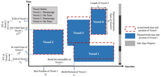
Figure 1.
A berthing plan for CBA.
In addition, we considered two essential features in this study: the tide time window and stochastic fluctuation of the vessels’ arrival time. Since most ports’ depth could not meet the draft requirements of all vessels, the port authority might ask the vessel to conduct its in-wharf and out-wharf operation in the tide time window. Hence, we introduced the tide time window, which meant that vessels could only in-wharf or out-wharf in specific time windows. The vessel’s berthing process in the tidal terminal is shown in Figure 2. Another feature of the proposed CBAP model is the uncertainty of vessels’ arrival time. Though vessel owners may provide their expected time of arrival (ETA), vessels usually delay due to the influence of uncertainty, e.g., the weather or a technical fault. Therefore, fluctuation exists in the arrival time of vessels and affects the overall objective value. As shown in Figure 2, the planned berth time and place of Vessel 1 and Vessel 3 were disrupted by delays which increased carbon emissions. Therefore, this paper introduces the RO theory to consider how to keep the minimizing objective value in the worst situation. In order to solve our BAP, we considered the following basic assumptions.
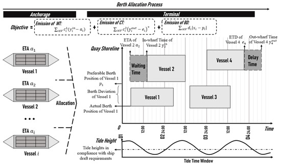
Figure 2.
Vessels berthing process in tidal terminal.
- The shoreline could be divided into several length units, and each vessel could berth at any position within the shoreline.
- Each vessel had a desirable position; deviating from this position would result in additional deviation costs.
- The planning period could be divided into several time units of equal length, and all vessels could only be in-wharf or out-wharf within the tide time window.
- The operation time of each vessel started from the berthing time until the departure time without interruption, and all arriving vessels could only be served once.
- The operation time of each vessel was known and could be completed on time.
- The vessel operation process was unaffected by external disturbances such as sudden vessel accidents or adverse weather conditions.
3.2. DBAP
This paper first introduces the deterministic berth allocation problem (DBAP). The mathematical mixed integer programming model could be formulated as follows.
The objective function (1) was to minimize the total emissions of WT, CT and BD. Objective (1) contained three parts: the first part was the weighted sum of all vessels’ emission of WT for in-wharf and berthing activity, the second part was the weighted sum of emissions with respect to the vessels’ CT, and the third part was the weighted sum of the emission of BD. Constraints (2)–(7) were the basic constraints for the CBAP. Constraint (2) ensured that each vessel could berth within the shoreline. Constraints (3) and (4) defined the order of vessels’ berthing position and time. Constraint (5) ensured that one vessel could only depart after completing its operation. Constraint (6) avoided time or position conflict between two vessels. Constraint (7) indicated that one vessel could only start its in-wharf process after its arrival. Constraints (8)–(13) were constraints on the tidal condition, which ensured that vessels’ in-wharf time and out-wharf time were in the tide time window. Constraints (12) and (13) ensured that each vessel could only berth or depart once during the tide time window. Constraints (14)–(18) were the domains of decision variables.
There were two non-linear forms and in objective (1). Replace the un-linearized part with and replace part with . Based on the above auxiliary variables, the linearized model was as follows:
s.t. Constraints (2)–(18).
3.3. TSROBAP
This section first constructs the general form of a TSRO model for the CBAP under uncertain vessel arrival time. Though the liners provide the port authority with an ETA, the actual arrival time could fluctuate due to uncertain conditions such as weather, port congestion, etc. Therefore, the port authority would require the crew to provide its arrival information according to the vessels’ position and navigation situation. The information provided by the crew was a relatively accurate time interval with higher reliability. According to the mentioned situation, this study considered the uncertainty of the vessel arrival time for vessel . We introduced an uncertain variable , , where represents the actual arrival time; is the fluctuation factor, ; is the perturbation of arrival time, , and is the disturbance ratio, .
In order to measure the possibility of conflicts between the two vessels, researchers usually introduce the concept of a time buffer, as proposed by Xu et al. [10]. In this study, the time buffer is represented by , as the difference between the in-wharf time of the following vessel and the out-wharf time of vessel . According to the definition of the time buffer, we should rewrite constraint (4). We introduced to identify vessels which may have conflicts, . In actual operations, the port authority could make a baseline schedule according to vessels’ ETA and calculate the corresponding . If , there is a conflict between vessel and the following vessels. Therefore, the port authority needs to improve the efficiency of the port to eliminate this conflict. This improvement could result in additional port operation equipment emissions, in the form of the recourse emissions of each vessel, denoted as . If ; this plan could be considered robust enough to deal with the fluctuation of uncertain arrival time, and there was no recourse emission. According to the definitions above, the could be presented as follows:
s.t. Constraints (2), (3) and (5)–(25),
The objective function (27) of this model aimed to minimize the total cost under the worst-case situation, including the baseline planning costs in the first stage and the recovery costs in the second stage. The cost of the baseline schedule for the first stage consisted of two parts: the first part of the corresponding objective function represented the emissions caused by the vessels’ WT and DT, and the second part represented the emissions of BD. The second stage was the recourse emissions of the delay caused by the uncertain arrival time of the vessels, which was the third part in the objective function (27). The maximum operator refers to the baseline allocation scheme that resulted in the maximum recourse emissions within the uncertainty set of the uncertain arrival time. The sum of the three-emission minimum operator can determine the final berth allocation plan with the minimum total emissions. Constraint (28) explained the time buffer, and Constraints (29)–(31) were the linearization function of .
In addition, a non-linearization item existed in Constraint (27). The un-linearized part could be replaced with , and could be used to linearize . Based on the above auxiliary variables, the linearized model was as follows:
s.t. Constraints (2), (3), (5)–(25) and (28)–(31).
The uncertain variable is contained in Constraint (33). There are generally two methods to describe it: uncertainty sets and scenarios. The former considers the continuous change in uncertain variables and uses different types of uncertainty sets to represent uncertain variables; the latter considers several scenarios to describe uncertain variables. Two ways are introduced and constructed in our two robust programming models: a TSROBAP-based uncertainty set (TSROBAP-US) and a TSROBAP-based scenario (TSROBAP-S).
3.3.1. TSROBAP-US
This section applies the uncertainty set to the classic robust optimization theory to describe . The robust counterpart could also be applied to formulate the TSROBAP-US. Firstly, standard uncertainty sets in robust optimization were introduced in this study, including box uncertainty sets, polyhedral uncertainty sets and ellipsoidal uncertainty sets. The box uncertainty set was the simplest form to solve, but it could easily lead to overly conservative solutions. A polyhedral uncertainty set was considered a particular form of an ellipsoidal set with linear structures, but it was difficult to reflect the correlation between uncertain parameters. The ellipsoidal uncertainty set could consider the probability of uncertainty occurrence to obtain better solutions, but this was harder to solve. Assuming the existence of an uncertain vector with elements, the form of the three uncertainty sets mentioned above could be represented as Formulas (36)–(38) [34,50,51]:
in which, , and represent the uncertain parameter of the box and polyhedral and ellipsoidal uncertainty sets, respectively, which can be used to control the uncertainty level. The robust Constraint (32) belongs to the right-hand side (RHS) type, and the basic form can be represented as Constraint (39):
in which, presents the parameter vector, denotes the decision variable, and is the true value after disruption. Constraint (39) could be transformed into Constraint (40) with formula
Combined with Formulas (36)–(38), Constraint (40) could be presented as follows,
in which could be replaced by , and according to the uncertainty set to be chosen. For the robust Constraint (32), the corresponding robust counterpart could be presented as:
in which, could be replaced by , and according to the uncertainty set to be chosen. With Constraint (42), the could be represented as follows,
s.t. Constraints (2), (3), (5)–(25), (28)–(31), (33)–(34) and (42).
The objective function (43) aimed to minimize the total emissions under worst-case situations, including the emissions of baseline planning in the first stage and the recourse emissions in the second stage. Similar to the objective functions (27) and (35), in function (43), the first part and second part included the decision emissions for the first stage, and the third part represented the recourse emissions for the second stage. The third part’s was selected according to the above three uncertainty sets, corresponding to the box uncertainty set , the polyhedral uncertainty set , and the ellipsoid uncertainty set , respectively. This part represented the allocation scheme that could result in maximum recourse emissions within the three uncertainty sets of an uncertain arrival time; that is, it corresponded with the worst-case situation.
3.3.2. TSROBAP-S
The scenario-based method is the most common tool for handling the BAP models under uncertainty [52]. This section uses scenarios as uncertainty factor descriptions to represent and construct models. The core idea of scenario-based robust programming is to assume a series of discrete scenarios to describe uncertainty. In this section, we assumed that the uncertainty set was known, in which represented the set of uncertain scenarios indexed by . The aforementioned could be transformed into based on uncertain scenarios:
s.t. Constraints (2), (3), (5)–(25) and (28)–(31).
The goal of the objective function (44) was to minimize the total emissions of the first and second stages under the worst scenario, which was similar to the objective function (27). Since the unlinearized form is contained in (44), we introduced positive variables to linearize , and used to replace .
The traditional scenario-based RO models had some of the following problems [26]. When the sets of uncertainties considered were too large (e.g., the RO problem included all possibilities), the solutions could be conservative, resulting in a high price for decision-making. Therefore, this study introduced a weight for the worst-case scenarios of each uncertain set and calculated the weighted sum of these uncertain sets. We adopted a data-driven method, the K-means clustering, which used data from the vessel’s Automatic Identification System (AIS) to construct uncertain scenario sets and search the worst-case scenario of . The process of K-means clustering has been added to Appendix B. The dataset was constructed by AIS alongside the schedule of liner companies. Next, K-means clustering was used to aggregate the dataset into non-overlapping sets, each of which could be considered as an uncertain scenario of the vessel arrival time. Then, we introduced the weight parameter , , and , which could be presented as:
s.t. Constraints (2), (3), (5)–(25), (28)–(31) and (45)–(47),
4. PSO Approaches
Since the proposed CBAP is an NP-hard problem, it is not easy to solve large-scale instances with CPLEX. Therefore, this paper could design a heuristic search method to solve the models mentioned above. Compared with other heuristic algorithms and machine learning approaches [53], the PSO algorithm could directly encode integers, and this was suitable for continuity problems to obtain an optimal solution faster [54]. Hence, we introduced the basic idea of PSO, and the variants investigated by Han et al. [55], Niu et al. [56], and Lu et al. [57] before making some improvements based on the above methods to solve our models. This paper investigated three improved PSO algorithms, including PSO, master-slave communication particle swarm algorithm (MCPSO), and expanded the master-slave communication particle swarm algorithm (EMCPSO) to handle the corresponding TSROBAP models. The improvements in our algorithms could be mainly described as follows:
- A virtual continuous time axis has been constructed by discrete-continuous transformation for the tide time window, which is suitable for PSO to enhance the solution efficiency;
- A first-come-first-service (FCFS) approach is proposed to provide an initial solution for PSO, which could further improve the convergence speed.
Section 4 is organized as follows: Section 4.1 describes the basic PSO algorithm and variants we refer to. Section 4.2 provides the solution representation and improvements of the PSO methods based on BAP. Initialize algorithm and example of the particles are presented in Section 4.3.
4.1. PSO Algorithms
This section describes the basic idea and framework of the PSO referred to by Han et al. [55] and two variants referred to by Niu et al. [56] and Lu et al. [57]. Assuming that a swarm contains particles, which are served as search agents for a specific problem solution, the position of each particle has dimensions, and the value of can be determined by the problem scale. The value of is the number of vessels in this study. The initial position for each particle is randomly generated. Each particle’s position can be considered a solution, and its fitness value can be calculated according to the objective function value. The fitness function is recorded as . Each particle has an individual best position, represented as , and the corresponding optimal value is . The optimal position obtained by the algorithm is the global best position, recorded as , and is the optimal value. For iterations, the speed and position on each dimension can be updated according to Formulas (50) and (51):
Among them, , and are defined parameters. Where can be regarded as an inertia of the particle, and to determine the learning weights of the individual and global optimal, where and are random numbers generated in the range of . The searching process of the PSO algorithm is shown in Figure 3. The speed of the particle in the iteration is determined by , and , which are also the three items in Formula (50).
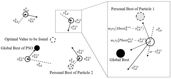
Figure 3.
Searching process of PSO algorithm.
According to the above formulas and process, the pseudocode of PSO algorithm is shown in Algorithm 1.
| Algorithm 1: Particle Swarm Optimization |
| ///* INITIALIZATION PROCESS START */// For each particle For each dimension Initialize position randomly within the permissible range Initialize velocity randomly within the permissible range |
| ///* INITIALIZATION PROCESS END */// Iteration While maximum iterations or stop criterion is satisfied. ///*ITERATION PROCESS START*/// For each particle Calculate fitness value If fitness value is better than in history Set the current fitness value as the Choose the particle having the best fitness value as the For each particle For each dimension Calculate velocity according to the Formula (50) Update particle position according to the Formula (51) ///*ITERATION PROCESS END*/// Output |
The main disadvantage of the traditional PSO algorithm is that it tends to converge too fast and fall into a locally optimal solution. Given the above problem, this paper introduced the MCPSO algorithm. The MCPSO adopted in this research could refer to Niu et al. [56]. In this approach, a particle population consists of one master swarm and several slave swarms. The symbiotic relation-vessel between the master swarm and slave swarms can keep the right balance in exploration and exploitation, which are essential for the success of a given optimization task. Master-slave communication is used to assign fitness evaluations and maintain algorithm synchronization. Each salve swarm executes a single PSO algorithm or its variants, including the velocity update, and creates a new population. When all the slave swarms are ready with new generations, each slave swarm then sends the best local individual position to the master swarm. This study considered the MCPSO algorithm with one master swarm () and slave swarm (). For iterations, the speed on each dimension was updated according to Formula (53):
in which, is a migration factor and is the best global optimal position. For a minimization problem, can be given by,
The overall procedure of MCPSO is described in Algorithm 2.
| Algorithm 2: Master-slave Communication PSO |
| ///* INITIALIZATION PROCESS START */// For each particle For each dimension For each Slave Swarm Initialize position randomly within the permissible range Initialize velocity randomly within the permissible range Run initialization process for master swarm Iterator ///* INITIALIZATION PROCESS END */// ///*ITERATION PROCESS START */// While maximum iterations or stop criterion is satisfied For each Slave Swarm Run iteration process in Algorithm 1 for slave swarm according to the Formula (52) Run iteration process in Alogorithm 1 for master swarm according to the Formula (52) For particle in master swarm and slave swarm. If Update the velocity and position using Formula (52) above, respectively ///* ITERATION PROCESS END */// |
| Output |
The EMCPSO algorithm [57] we referred to is an improvement of the MCPSO [56]. Lu et al. [57] proposed that when a sub-swarm falls into the local optimum, misinformation spreads quickly among the population, increasing the risk of premature convergence. Therefore, adopting a proper cooperating approach when using the multi-swarm technique is crucial. In the case of settling the above problem, Lu et al. [57] introduced a stagnation check for the original MCPSO to avoid it falling into a locally optimal solution. The stagnation check forced the particles to escape from the optimal local solution after a certain number of times and carried on a global search. The checker was denoted by for each slave swarm . During the iteration, when the optimal global value of each slave swarm was unchanged, . When was greater than the parameter we were given in advance, the slave swarm was executed to jump out of the optimal local solution.
For this stagnation check measure, a probability was first given. When the generated random number was less than this probability , the position of this point changed to a new value within the range of random feasible solutions, as shown in the formula: . When the randomly generated random number was larger than this probability interval, took the position of and in proportion to , . It could be seen from the structure that when the global search ability of the algorithm needed to be guaranteed, a smaller and a larger could be set, and when the algorithm needed to converge quickly, a larger and a smaller were required. In addition, represented the variance of the optimal value of the slave swarm in each iteration, which could be calculated as follows for the iteration:
The pseudocode of EMCPSO is shown in Algorithm 3.
| Algorithm 3: Enhanced Master-slave Communication PSO |
| ///* INITIALIZATION PROCESS START */// Initialize populations (Initialization Process in Algorithm 2) Iterator Run initialization process for master swarm Iterator ///* INITIALIZATION PROCESS END *//////*ITERATION PROCESS START */// While maximum iterations or stop criterion is satisfied, For each Slave Swarm Run iteration process in Algorithm 1 for slave swarm according to the Formula (53) Run iteration process in Alogorithm 1 for master swarm according to the Formula (53) For particle in master swarm and slave swarm If ///* STAGNATION CHECKER START*/// For each Slave Swarm If If For each dimension If Else Else ///* STAGNATION CHECKER END*/// Update the velocity and position of the using Formula (52) above, respectively ///* ITERATION PROCESS END */// |
| Output |
4.2. Solution Representation
Apart from the algorithms mentioned above, several developments were conducted due to the characteristics of the proposed model. Based on Guo et al. [58], PSO was more suitable for continuous problems. Since the tide time window was considered in our model, it was not suitable for the particles to perform a continuous movement in the iterative process, which could affect the efficiency of the algorithms. Therefore, this paper introduced the concept of the virtual time axis and actual time axis to improve the original algorithms. The length of the actual time axis was the original planning period. Since this article considered the tide time window, the actual time axis was divided into several time intervals, as shown in Figure 4. A particle was searched on the actual time axis, but due to the continuity of particle motion, this particle inevitably entered the low tide time window. The vessel could not complete the in-wharf and out-wharf process in this non-tidal time window, resulting in invalid iterations. This situation is shown in the position of and in the actual time axis within Figure 4. These invalid iterations affected the convergence efficiency of the algorithms. This study solved this problem by introducing the virtual time axis. For each vessel, the corresponding tide time length was . As shown in Figure 5, the non-tidal time window was removed from the actual time axis, and the feasible tide time window was retained as the virtual time axis.
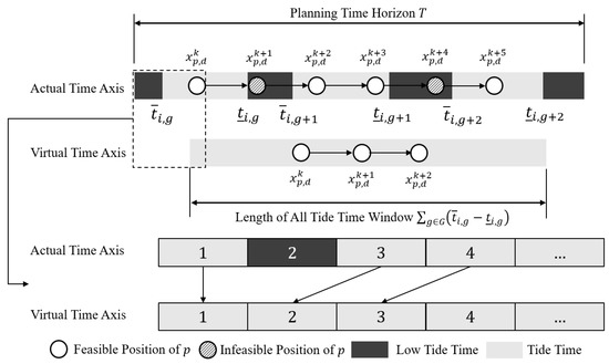
Figure 4.
Presentation of virtual time axis.
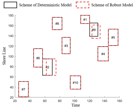
Figure 5.
Solutions of deterministic model and robust model.
4.3. Population Initialization
In addition to the above improvements, the initialization process of PSO (see Algorithms 1–3 for detailed steps) also played a vital role in the algorithm’s efficiency. In order to avoid invalid iterations and an uncertain solution time generated by the arbitrary initial solution generation rule, this paper made some restrictions to the feasible space of initial solution generation to reduce the iterative steps of the algorithm.
- For any vessel , the berth position was generated , , where refers to a random number.
- For any vessel , the left bound and upper bound of its berth time on the actual time axis should be . Due to the possibility that the vessel arrival time might not fall within the tide time window and the large range of the upper bound of , we, therefore, considered the nearest tide time window’s start time and end time to as the upper and lower bounds for the generated variable .
For any vessel , the left bound and upper bounds of the departure time on the actual time axis should be . However, due to the possibility that might not fall within the tie time window and the issue of a potentially large range of the upper bound of , we considered the nearest tie time window’s start time and end time to as the upper and lower bounds for the generated departure time .
In addition to particle generation, the initial position played a crucial role in guiding the convergence of the PSO algorithm; it directly influenced the velocity update direction of all particles, as observed in Equations (51)–(53). Therefore, this paper introduced the FCFS algorithm to generate a feasible solution that served as the initial global best solution for the PSO algorithm. The steps of FCFS are presented as follows:
- According to the arrival time of vessel , calculate the earliest in-wharf time window and denote it as the vessel’s berth time .
- According to the berth time and operation time of vessel , calculate the earliest out-wharf time window and denote it as the vessel’s depart time .
- The berth position of vessel is generated as follows. Sort the vessels in the order of arrival time from the berth position 0. When berth position exceeds the difference between berth length and the max vessel length , the berth position can be generated again from position 0.
5. Numerical Experiment
Extensive numerical experiments were conducted to validate the performance of the proposed models and algorithms. The model validation of the experiment was performed by invoking the CPLEX 12.10 solver through programming and solving in C++ (Visual Studio). This algorithm was implemented using Python 3.8 for relevant program development. All written programs were executed and processed on a PC with the following configuration: 3.60 GHz Intel(R) Core™ i7-12700K CPU and 32 GB DDR4 2666 MHz RAM. Section 5 was organized as follows: Section 5.1 describes how to generate the instances; Section 5.2 compares different models; Section 5.3 provides an algorithm comparison; Section 5.4 takes the sensitivity analysis.
5.1. Instance Generation
Instance-Related Parameters. The planning horizon . The shoreline length was with a unit length of 10 m. The length of vessel was denoted as , . The operation time of vessel was denoted as , . The ETA was , . The was generated according to the following rules: , in which . The expected berth position was . The three emission coefficients , , and , were randomly generated integers within the range . The table of the tide time window used in this study was compiled based on publicly available information. It was derived from the tidal height data of Shanghai Yangshan Port from 1 February 2023 to 7 February 2023. We considered a randomly generated integer within the range of for the vessel draft. Correspondingly, the arrival and departure time window could be calculated based on the draft and the tide time window, as shown in Appendix C.
Uncertainty-Related Parameters. The recourse emission was . The uncertainty set was determined by comparing the historical actual arrival information of domestic liner routes with the ETA data provided by liner companies in their vessel schedules. The AIS data were sourced from Vesselxy, which contained the navigation records of the majority of domestic vessels. The ETA data for vessels were sourced from the Pan Asia Vesselping Schedule. The data used in this study covered the time range from 1 February 2023 to 7 February 2023. In the models based on the box set , the polyhedral set , and ellipsoid set , we excluded outliers (i.e., consider 90% of the voyage records) and rounded the values. We calculated that the fluctuation range in the vessel’s arrival time was approximately within a range of plus or minus 5 h. Therefore, we set the uncertainty level parameter at five for the three uncertainty sets, i.e., . In the model based on uncertain scenarios, we calculated the uncertainty set based on Constraints (47) and (50). We used the K-means clustering data-driven method to aggregate scenarios, resulting in a total of uncertain scenarios. The sample set was constructed from the fluctuation values of the arrival time and preprocessed using AIS data and the Pan Asia Vesselping Schedule for the period from 1 February 2023 to 7 February 2023.
PSO-Related Parameters. The algorithm parameter settings mentioned above are presented in Table 2. As for the termination criterion, this study stated that the algorithm would stop if the global best value remained unchanged after 60 iterations.
Table 2.
Parameter list for three particle swarm optimization algorithms.
For the problem scale, this study utilized a number of vessels as a parameter to control the scale of the problem instances. Four problem instances with different scales were considered, where the vessel quantities were chosen as and denoted as G1, G2, G3, and G4, respectively. Table 3 provides an overview of these problem instances.
Table 3.
The parameter configuration scale of numerical experimental instances.
5.2. Model Performance
5.2.1. Comparison with Deterministic Model
First, we compared the solutions obtained from the two-stage robust optimization and deterministic models. Figure 5 presents a schematic representation of the solutions obtained from the deterministic model and the two-stage extended robust model based on uncertain scenarios and considering an instance with 10 vessels. The solid black line represents the berth allocation results from the deterministic model. In contrast, the dashed red line segments represent the specific berth allocation scheme obtained from the two-stage extended robust model based on uncertain scenarios. Before comparing the algorithms, the solution results of different models were compared.
Figure 5 shows the solution results of an instance considering 10 vessels. The robustness of this model was verified by comparing the deterministic and robust models. The red dashed line is the specific assignment result obtained from the robust model, and the solid black line is the model result obtained from the deterministic model. As shown in Figure 6, the time buffer between the vessels obtained from the robust model was larger than the deterministic model. In addition, the robust model adjusted the specific vessel distribution (e.g., Vessel #2, Vessel #9) compared to the deterministic model. This was in order to cope with possible vessel conflicts. Again, this adjustment led to a large value in the objective function of the robust model.
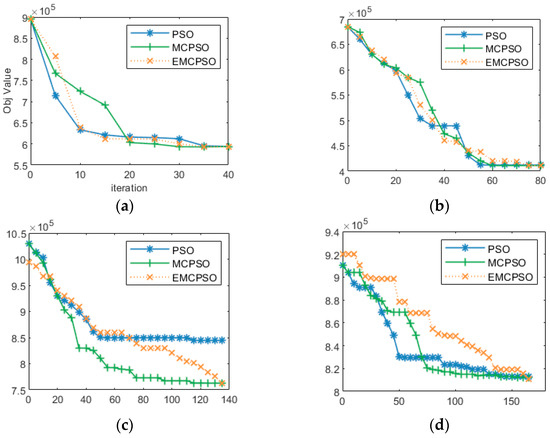
Figure 6.
Convergence of the three particle swarm optimization algorithms. Note: The horizontal axis indicates the number of iterations, and the vertical axis indicates the value of the objective function. (a) Results of solving Example G1-1; (b) Results of solving Example G2-1; (c) Results of solving Example G3-1; (d) Results of solving Example G4-1.
5.2.2. Comparison between Uncertain Models
In order to compare the two robust methods of constructing models, the concept of difference is introduced in this section. The deviation values of the objective function and the solution time are compared between the two models. The formulae are shown in Equations (54) and (55), respectively:
The case sizes G1, G2, G3, and G4 correspond to the number of vessels . For example, case number G1-1 represents the first case of 10 vessels. From the comparison of solution times, the EMCPSO extended the master-slave parallel collaborative PSO algorithm, which was used uniformly for model solutions. The time consumed by aggregating the uncertainty set and using the K-means clustering method in the first stage was separate from the subsequent solution time. Only the time used by the models in the solution phase was compared. The final comparison between the two robust models in terms of objective function values and solution times is shown in Table 4 below.
Table 4.
Comparison of two robust solution times and objective functions.
When comparing the objective function values, the values of the model were lower than those of the model. The deviation value Diff 1 between them was in the range . Based on this result, there was no significant difference in the objective function values between the two two-stage robust planning models.
In the comparison of the solution time, the solution time of the model differed from the solution time deviation value Diff 2 of the model within the range . The value of this deviation value fluctuated widely. Based on this result, there was no significant computation time pattern between the two-stage robust planning models.
5.3. Algorithm Peroformance
5.3.1. Comparison with CPLEX
In this section, the validation of the models studied in this chapter was carried out by the CPLEX solver. The solution results are shown in Table 5. Meanwhile, the TSRO models’ experiment with the three PSO algorithms was used to evaluate the performance of the improved algorithms. This section mainly compares the final objective function values, the solution time, and the iteration efficiency.
Table 5.
Numerical experimental results of robust models of CPLEX, PSO, MCPSO and EMCPSO for solving different problem case sizes.
In addition, since the initial particles of the particle swarm optimization algorithm were randomly generated, it led to a certain degree of randomness in performance fluctuations during the algorithm’s operation. Therefore, in this study, to eliminate the fluctuations caused by the initialization of particles to some extent, we computed each arithmetic case three times. Moreover, the three times calculated for each algorithm’s arithmetic case were taken as the average value for the final algorithm performance. In order to present these conclusions intuitively, the concept of Gap was introduced in this study to measure the accuracy difference between the three particle swarm optimization algorithms and the CPLEX solution results. The gap was calculated as shown in the following equation.
Based on these results in Table 5, we can draw several conclusions as follows:
The CPU time used to solve the proposed models using PSO, MCPSO and EMCPSO was much faster than that used to solve the models directly by CPLEX. When the problem size of instances became larger, the CPU time of CPLEX also increased rapidly. In contrast, the CPU time for solving the models remained relatively stable for the three PSO algorithms.
The performance of three different PSO algorithms is compared. PSO was more efficient and advantageous in small problem sizes. MCPSO and EMCPSO performed better on medium and larger problem sizes, while MCPSO demonstrated a faster solution speed, and EMCPSO had a higher solution accuracy.
Due to the algorithms’ limitations, PSO could fall into local optimum solutions. For example, in cases G3-1 and G4-2 of Table 5, the optimal solutions solved by PSO had a gap value greater than 10% compared with the target value obtained by CPLEX. For MCPSO, there was also the case of falling into an optimal local solution, as shown in example G3-2 of Table 5. However, EMCPSO did not fall into a locally optimal solution in the test data. Therefore, EMCPSO performed better in finding the global optimum. Due to the stagnation check mechanism, the optimal solutions found by EMCPSO were generally the most similar compared to the value obtained by CPLEX.
To calculate the iterative efficiency, the first group of each algorithm (i.e., G1-1, G2-1, G3-1, and G4-1) was chosen to observe its convergence rate. We took the optimal value of every five iterations for a more straightforward presentation. The specific results are shown in Figure 6.
The number of iterations in the figure was interpreted: as the number of iterations when the last of the three PSO algorithms reached the global optimum for the first time. For example, the results in Figure 6a are selected at 40 iterations because the number of iterations when the EMOCPSO algorithm with the slowest solution result reached the global optimum for the first time was 42, and the value of 40 iterations was taken for display. Combining Figure 6 with the final values in Table 5 shows that the basic PSO algorithm had the fastest iterative convergence rate overall. However, it tended to fall into local optimal solutions, affecting the efficiency of the algorithm. As shown in Figure 6b, the trend of the solution results of PSO was between 40 and 50 iterations, and in Figure 6d, the trend of the solution results was after 50 iterations. For EMCPSO, particles could jump out of the local optimal solution. This phenomenon was particularly evident for the large problem size. Figure 6d shows three instances of jumping out of the EMCPSO algorithm after falling into a local optimum. Moreover, the optimal solution result was finally obtained.
5.3.2. Comparison with Traditional PSO
Compared with the traditional PSO, two main improvements (virtual time axis and FCFS generation) were considered in this paper. The comparison in this section could also be measured regarding the specific performance of these two improvements. Moreover, a comparison was made regarding the number of iteration steps and the CPU time.
For the virtual time axis, the comparison results of the subgroups are shown in Figure 7. Since the concept of a virtual time axis aims to reduce the number of iteration steps in the algorithm, Figure 7a–d shows the number of iterations for instances G1-1, G2-1 and G3-1, G4-1, respectively. Among these, an unimproved algorithm with 200 iterations appeared in Figure 7c,d. This case meant that the number of iterations in the algorithm exceeded the upper limit. Moreover, the Gap between the final and CPLEX solution result was more than 30%. From Figure 7a,b, the virtual time axis reduced the number of iterations in the algorithm by about 50%. This could significantly improve the efficiency of the algorithm.
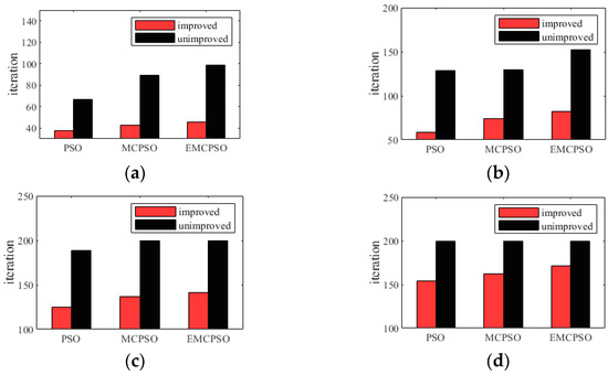
Figure 7.
Virtual time axis efficiency assessment. Note: The vertical axis represents the number of iterations. (a) Solution result of calculation example G1-1; (b) Solution result of calculation example G2-1; (c) Solution result of calculation example G3-1; (d) Solution result of calculation example G4-1.
For the FCFS method comparison, the best position of the initially generated cluster was compared to the global optimum. To improve FCFS, it provided an initial optimal solution that was a better feasible solution for all particles in the swarm. Therefore, its main contribution was to save the overall solving time of the algorithm. Similarly, the comparison of CPU time is shown in Figure 8. It shows that the solution time of the algorithms with the FCFS improvement was significantly less than that of the algorithms without FCFS improvement. For each type of PSO, the strategy of FCFS to generate the initial solution could effectively reduce the CPU time of the algorithms. The algorithm improvement proposed in this paper is, therefore, significantly beneficial.
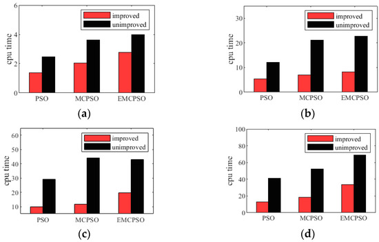
Figure 8.
FCFS efficiency evaluation of the initial solution. Note: The vertical axis represents the solution time. (a) Solution result of calculation example G1-1; (b) Solution result of calculation example G2-1; (c) Solution result of calculation example G3-1; (d) Solution result of calculation example G4-1.
5.4. Sensitivity Analysis
For the disturbance of uncertain factors, different TSRO models could be affected to different degrees and correspondingly produce different amplitudes. In order to evaluate the robustness of the TSRO models and the effectiveness of the solution methods, this section first studies the impact of the degree of uncertainty in the container loading and unloading time on the decision-making of , and then studies the fluctuation in the number of uncertain scenarios that could affect the model. The sensitivity analysis in this section mainly compares the objective function values of different models.
To evaluate the effectiveness and the model’s robustness, this section examines how the handle time uncertainty affected our decisions. We compared the and robust model . Moreover, carried out a sensitivity analysis of the vessel’s container loading and unloading operation time hi. We introduced the sensitivity analysis parameter , and considered the variation in the objective function value and the buffer time mean value . The sensitivity analysis results are shown in Figure 9. The objective function values of the two models increased when the perturbation in the container handling operation time of the vessel increased. Unlike the deterministic model, the robust model might have a situation where the objective function value remains constant. This phenomenon was observed for all four case sizes, as shown in Figure 9a–d. This phenomenon showed that the solution results of the TSRO model itself could cope with the particular risk of uncertainty fluctuations.
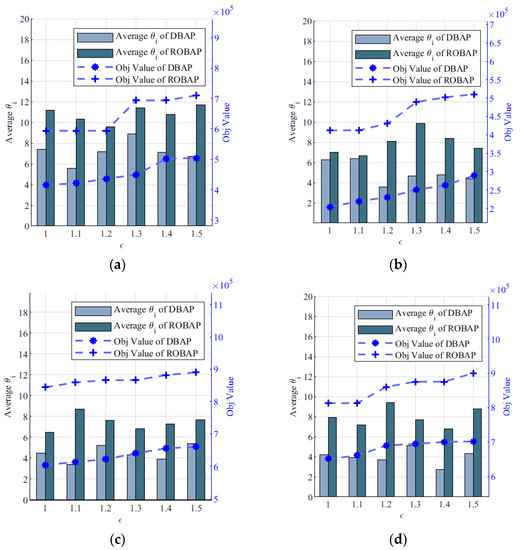
Figure 9.
Sensitivity analysis results. Note: The left vertical axis indicates the mean buffer time . The right vertical axis indicates the objective function value. The horizontal axis indicates the sensitivity analysis parameters . (a) Results of solving Example G1-1; (b) Results of solving Example G2-1; (c) Results of solving Example G3-1; (d) Results of solving Example G4-1.
In addition, the assessment of the buffer time meant that was also a critical factor in evaluating the solution’s risk resistance. From Figure 9, the mean buffer time of the deterministic model was significantly smaller than that of the robust model . Although a shorter buffer time brought a smaller value to the objective function, the solution of the deterministic model could also be subject to the risk of fluctuation due to higher uncertainty.
The number of scenes is an essential parameter in the scenario-oriented model. This parameter directly affects the final result of the objective function. To evaluate the impact of the number of uncertain scenarios on the final results of the model, this paper considered the variation in the objective function when the number of uncertain scenarios was, i.e., . The results of this analysis are shown in Figure 10. In terms of trend, when the number of scenarios increased, the function value gradually decreased. The reason for this phenomenon was that when the number of uncertainties increased, the probability of the worst scenario was more accurate. In other words, more uncertain scenarios could accurately identify the probability of each worst-case and give a more accurate weight . At the same time, it gave a smaller robust solution to the objective function.
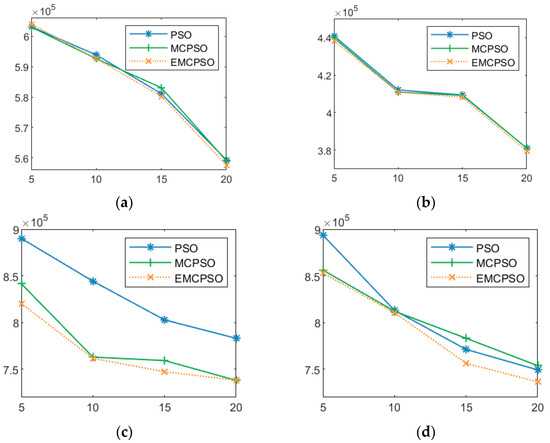
Figure 10.
Results of analysis of fluctuations in the number of uncertain scenarios. Notes: (a) Results of solving Example G1-1; (b) Results of solving Example G2-1; (c) Results of solving Example G3-1; (d) Results of solving Example G4-1.
6. Conclusions
In this paper, the CBAP considered the tide time window and uncertain arrival time. A variety of three improved PSO algorithms were used to solve the models. At the same time, several improved methods for PSO were created, and numerical examples of different instances were used to verify the effectiveness of the algorithm. The main results of this paper are as follows:
- A deterministic MIP model can be constructed to solve the CBAP under tidal conditions, aiming to minimize the carbon emissions caused by waiting time, consumed time and the deviation to berth preference.
- According to real situations in the daily operation of the terminal, this study took vessels’ arrival time as the uncertainty factor to formulate the models. The results have practical significance.
- Both the uncertainties sets and uncertain scenarios were considered in this paper to construct the two-stage robust optimization models. Robust counterpart constraints were applied to transfer the deterministic MIP model into robust programming models according to corresponding theories.
- Three different improved PSO algorithms with enhancements were used to solve the mentioned problems. The characteristics were summarized through the comparison between the algorithms. This contribution could provide a reference for subsequent scholars engaged in related fields.
- The variance in the objective value of the robust models, when the uncertainty fluctuates, is compared. Based on the results, our models have a certain ability to resist unknown risks.
However, this study also has several limitations. For example, there are occasionally extreme uncertainty situations in real life, such as the inability of the vessel to berth or a change in the port of call. The occurrence of this situation would also have a significant impact on the daily operation of the port. There are more uncertain parameters that could affect the BAP, such as facilities interruption, channel capacity, weather conditions, etc. In addition, the port and academic community could also gradually shift their focus to other sources of terminal carbon emissions. These will become the focus of our future research.
Author Contributions
All the authors contributed to the conceptualization, formal analysis, investigation, methodology, and writing (original draft, review, and editing). All authors have read and agreed to the published version of the manuscript.
Funding
This study is supported by the Shanghai philosophy and social science fund under grant 2022ZGL005.
Institutional Review Board Statement
Not applicable.
Informed Consent Statement
Not applicable.
Data Availability Statement
The data developed in this study will be made available upon request to the corresponding author.
Acknowledgments
We would like to express our sincere gratitude to the editor and anonymous referees for their insightful and constructive comments that substantially improved this paper. In addition, we would like to express our deep gratitude to the our colleagues at Shanghai University of Engineering Science for their helpful and constructive suggestions.
Conflicts of Interest
The authors declare no conflict of interest.
Abbreviations
| Indices, Sets and Parameters | |
| set of vessels, indexed by and . | |
| set of planning time, indexed by . | |
| set of tide cycles, indexed by . | |
| length of the shoreline. | |
| vessel length of vessel . | |
| operation time of vessel . | |
| preferable berthing position of vessel . | |
| estimated arrival time of vessel . | |
| latest shore power using time of vessel . | |
| emission index of auxiliary machine of vessel in waiting time. | |
| emission index of auxiliary machine of vessel in consuming time. | |
| the cost of berth deviation of vessel . | |
| berthing time window for vessel in the tide. | |
| a sufficiently large positive number. | |
| Decision Variable | |
| integer, represents the berthing position of vessel . | |
| integer, berthing time of vessel . | |
| integer, departure time of the vessel . | |
| binary, equals one if vessel berths on the left of vessel , and zero otherwise. | |
| binary, equals one if vessel berths before vessel , and zero otherwise. | |
| binary, equals one if in-wharf time of vessel is in the berthing time window of the tide cycle. | |
| binary, equals one if out-wharf time of vessel is in the departing time window of the tide cycle. | |
Appendix A. Acronyms of Table 1
We followed the considered type of layout provided by Bierwirth and Meisel [14]: discrete (D) and continuous (C). We identified the two most common uncertain parameters, i.e., arrival time (AT) and operation time (OT). For the decision variable, we identified the three most common items, i.e., berthing time (BT), departure time (DT) and berth position (BP). The service level of the ports, waiting time (W), was the difference between the expected arrival time and the actual berthing time of the vessel; handling time (H), which is also known as the operation time, corresponded to the difference between the starting time and the ending time of the operation of vessel; completion time (C) corresponded to the difference between the vessel’s arrival time and its ending time of the operation; tardiness (T) was the delay caused by a larger completion time than the expected time of departure; deviation from desirable berth position (P), corresponded to either a deviation from a lower cost position or previously arranged position. We considered two common models to solve the uncertain problem, including stochastic programming (SP) and robust optimization (RO). We identified the solution algorithms used for solving the problem. The operator ‘+’ means a combination of methods; the operator ‘A(B)’ means that method ‘B’ is used inside ‘A’; the operator ‘,’ indicates the use of independent methods; and the operator ‘A → B’ indicates that method ‘A’ is used to obtain ‘B’. Acronyms: SA—simulated annealing; B&B—branch-and-bound; EA—evolutionary algorithm; PFE—Pareto front estimation; MCS—Monte Carlo simulation; HA—heuristic algorithm; GWO—grey wolf optimization; LS—local search; RCEH—recovery cost estimation heuristic; SOH—simulation-optimization heuristic; RHH—rolling horizon heuristic; C&CG—column-and-constraint generation; PSO—particle swarm optimization; GA—genetic algorithm; ML—machine learning.
Appendix B. K-Means Clustering
| Algorithm A1: K-Means Clustering |
| Input: Data Set , Number of Centroids , |
| ///* INITIALIZATION PROCESS START */// Choose points in as centroids ///* K-MEANS PROCESS START */// While ( remains unchanged) For point in For centroid Calculate the distance from to End For Put into with the shortest End For For centroid in : Update according to End For ///* K-MEANS PROCESS END */// Output: position of centroids , clustering sets , where |
Appendix C. Tide Time Window
The tide time window used in this study was compiled according to the public information of Shanghai Yangshan Port from 1 February 2023 to 7 February 2023.
| Planning | D1 | D2 | D3 | D4 | D5 | D6 | D7 | |
| Tide | ||||||||
| 0 | 153 | 205 | 265 | 322 | 368 | 394 | 404 | |
| 1 | 129 | 159 | 206 | 262 | 316 | 362 | 394 | |
| 2 | 126 | 126 | 147 | 189 | 241 | 293 | 339 | |
| 3 | 148 | 116 | 108 | 122 | 158 | 207 | 258 | |
| 4 | 195 | 133 | 94 | 81 | 93 | 124 | 169 | |
| 5 | 254 | 178 | 113 | 70 | 55 | 65 | 96 | |
| 6 | 314 | 245 | 166 | 99 | 53 | 35 | 45 | |
| 7 | 361 | 318 | 250 | 172 | 102 | 52 | 28 | |
| 8 | 386 | 377 | 339 | 276 | 200 | 130 | 75 | |
| 9 | 386 | 409 | 404 | 372 | 319 | 251 | 182 | |
| 10 | 360 | 412 | 436 | 433 | 409 | 367 | 312 | |
| 11 | 315 | 383 | 433 | 457 | 457 | 439 | 409 | |
| 12 | 263 | 329 | 392 | 439 | 465 | 470 | 459 | |
| 13 | 214 | 265 | 325 | 382 | 427 | 455 | 468 | |
| 14 | 177 | 203 | 248 | 301 | 353 | 396 | 427 | |
| 15 | 157 | 154 | 178 | 218 | 264 | 310 | 352 | |
| 16 | 160 | 127 | 125 | 148 | 183 | 223 | 262 | |
| 17 | 189 | 128 | 97 | 97 | 118 | 149 | 183 | |
| 18 | 233 | 167 | 110 | 78 | 74 | 90 | 116 | |
| 19 | 275 | 227 | 170 | 116 | 77 | 62 | 67 | |
| 20 | 303 | 284 | 248 | 200 | 149 | 102 | 68 | |
| 21 | 310 | 321 | 315 | 290 | 250 | 201 | 148 | |
| 22 | 293 | 332 | 350 | 352 | 338 | 306 | 261 | |
| 23 | 253 | 312 | 355 | 378 | 384 | 377 | 354 | |
References
- Mehregan, E. Designing a sustainable development model with a dynamic system approach. NeuroQuantology 2022, 20, 8143–8164. [Google Scholar]
- Kler, R.; Gangurde, R.; Elmirzaev, S.; Hossain, M.S.; Vo, N.V.; Nguyen, T.V.; Kumar, P.N. Optimization of Meat and Poultry Farm Inventory Stock Using Data Analytics for Green Supply Chain Network. Discret. Dyn. Nat. Soc. 2022, 2022, 8970549. [Google Scholar] [CrossRef]
- Dang, T.-T.; Nguyen, N.-A.-T.; Nguyen, V.-T.-T.; Dang, L.-T.-H. A Two-Stage Multi-Criteria Supplier Selection Model for Sustainable Automotive Supply Chain under Uncertainty. Axioms 2022, 11, 228. [Google Scholar] [CrossRef]
- Jiang, M.; Feng, J.; Zhou, J.; Zhou, L.; Ma, F.; Wu, G.; Zhang, Y. Multi-Terminal Berth and Quay Crane Joint Scheduling in Container Ports Considering Carbon Cost. Sustainability 2023, 15, 5018. [Google Scholar] [CrossRef]
- Global CO2 Emissions from Transport by Sub-Sector in the Net Zero Scenario, 2000–2030 [EB/OL]. [2020-11-16]. Available online: https://www.iea.org/data-and-statistics/charts/global-co2-emissions-from-transport-by-sub-sector-in-the-net-zero-scenario-2000-2030 (accessed on 22 September 2022).
- Zhen, L.; Sun, Q.; Zhang, W.; Wang, K.; Yi, W. Column Generation for Low Carbon Berth Allocation under Uncertainty. J. Oper. Res. Soc. 2021, 72, 2225–2240. [Google Scholar] [CrossRef]
- Peng, Y.; Wang, W.; Liu, K.; Li, X.; Tian, Q. The Impact of the Allocation of Facilities on Reducing Carbon Emissions from a Green Container Terminal Perspective. Sustainability 2018, 10, 1813. [Google Scholar] [CrossRef]
- Qu, S.; Shu, L.; Yao, J. Optimal Pricing and Service Level in Supply Chain considering Misreport Behavior and Fairness Concern. Comput. Ind. Eng. 2022, 174, 108759. [Google Scholar] [CrossRef]
- He, Q.; Xia, P.; Hu, C.; Li, B. Public Information, Actual Intervention and Inflation Expectations. Transform. Bus. Econ. 2022, 21, 644–666. [Google Scholar]
- Xu, Y.; Chen, Q.; Quan, X. Robust Berth Scheduling with Uncertain Vessel Delay and Handling Time. Ann. Oper. Res. 2012, 192, 123–140. [Google Scholar] [CrossRef]
- Sheikholeslami, A.; Iiati, G.; Kobari, M. The Continuous Dynamic Berth Allocation Problem at a Marine Container Terminal with Tidal Constraints in the Access Channel. Int. J. Civ. Eng. 2014, 12, 344–353. [Google Scholar]
- Segura, F.G.; Segura, E.L.; Moreno, E.V.; Uceda, R.A. A Fully Fuzzy Linear Programming Model to the Berth Allocation Problem. In Proceedings of the 2017 Federated Conference on Computer Science and Information Systems (FedCSIS), Prague, Czech Republic, 3–6 September 2017; pp. 453–458. [Google Scholar]
- Guo, L.; Zheng, J.; Du, H.; Du, J.; Zhu, Z. The Berth Assignment and Allocation Problem Considering Cooperative Liner Carriers. Transp. Res. Part E Logist. Transp. Rev. 2022, 164, 102793. [Google Scholar] [CrossRef]
- Bierwirth, C.; Meisel, F. A Survey of Berth Allocation and Quay Crane Scheduling Problems in Container Terminals. Eur. J. Oper. Res. 2010, 202, 615–627. [Google Scholar] [CrossRef]
- Bierwirth, C.; Meisel, F. A follow-up survey of berth allocation and quay crane scheduling problems in container terminals. Eur. J. Oper. Res. 2015, 244, 675–689. [Google Scholar] [CrossRef]
- Rodrigues, F.; Agra, A. Berth allocation and quay crane assignment/scheduling problem under uncertainty: A survey. Eur. J. Oper. Res. 2022, 303, 501–524. [Google Scholar] [CrossRef]
- Ting, C.-J.; Wu, K.-C.; Chou, H. Particle swarm optimization algorithm for the berth allocation problem. Expert Syst. Appl. 2014, 41, 1543–1550. [Google Scholar] [CrossRef]
- Agra, A.; Oliveira, M. MIP approaches for the integrated berth allocation and quay crane assignment and scheduling problem. Eur. J. Oper. Res. 2018, 264, 138–148. [Google Scholar] [CrossRef]
- Xiang, X.; Liu, C.; Miao, L. Reactive strategy for discrete berth allocation and quay crane assignment problems under uncertainty. Comput. Ind. Eng. 2018, 126, 196–216. [Google Scholar] [CrossRef]
- Hendriks, M.; Laumanns, M.; Lefeber, E.; Udding, J.T. Robust cyclic berth planning of container vessels. OR Spectr. 2010, 32, 501–517. [Google Scholar] [CrossRef]
- Mauri, G.R.; Ribeiro, G.M.; Lorena, L.A.N.; Laporte, G. An adaptive large neighborhood search for the discrete and continuous berth allocation problem. Comput. Oper. Res. 2016, 70, 140–154. [Google Scholar] [CrossRef]
- Kim, K.H.; Moon, K.C. Berth scheduling by simulated annealing. Transp. Res. Part B Methodol. 2003, 37, 541–560. [Google Scholar] [CrossRef]
- Sheikholeslami, A.; Ilati, R. A sample average approximation approach to the berth allocation problem with uncertain tides. Eng. Optim. 2018, 50, 1772–1788. [Google Scholar] [CrossRef]
- Zhen, L.; Liang, Z.; Zhuge, D.; Lee, L.H.; Chew, E.P. Daily berth planning in a tidal port with channel flow control. Transp. Res. Part B Methodol. 2017, 106, 193–217. [Google Scholar] [CrossRef]
- Hsu, H.-P.; Chiang, T.-L.; Wang, C.-N.; Fu, H.-P.; Chou, C.-C. A Hybrid GA with Variable Quay Crane Assignment for Solving Berth Allocation Problem and Quay Crane Assignment Problem Simultaneously. Sustainability 2019, 11, 2018. [Google Scholar] [CrossRef]
- Xiang, X.; Liu, C. An expanded robust optimisation approach for the berth allocation problem considering uncertain operation time. Omega 2021, 103, 102444. [Google Scholar] [CrossRef]
- Xiang, X.; Liu, C. An almost robust optimization model for integrated berth allocation and quay crane assignment problem. Omega 2021, 104, 102455. [Google Scholar] [CrossRef]
- Zhen, L.; Zhuge, D.; Wang, S.; Wang, K. Integrated berth and yard space allocation under uncertainty. Transp. Res. Part B Methodol. 2022, 162, 1–27. [Google Scholar] [CrossRef]
- Golias, M.; Portal, I.; Konur, D.; Kaisar, E.; Kolomvos, G. Robust berth scheduling at marine container terminals via hierarchical optimization. Comput. Oper. Res 2014, 41, 412–422. [Google Scholar] [CrossRef]
- Ursavas, E.; Zhu, S.X. Optimal policies for the berth allocation problem under stochastic nature. Eur. Oper. Res. 2016, 255, 380–387. [Google Scholar] [CrossRef]
- Liu, C.; Xiang, X.; Zheng, L. Two decision models for berth allocation problem under uncertainty considering service level. Flex. Serv. Manuf. J. 2017, 29, 312–344. [Google Scholar] [CrossRef]
- Soyster, A.L. Convex programming with set-inclusive constraints and application to inexact linear programming. Oper. Res. 1973, 21, 1154–1157. [Google Scholar] [CrossRef]
- Ben-Tal, A.; Nemirovski, A. Robust solutions of uncertain linear programs. Oper. Res. Lett. 1999, 25, 1–13. [Google Scholar] [CrossRef]
- Bertsimas, D.; Sim, M. The price of robustness. Oper. Res. 2004, 52, 35–53. [Google Scholar] [CrossRef]
- Ji, Y.; Ma, Y. The Robust Maximum Expert Consensus Model with Risk Aversion. Inf. Fusion 2023, 99, 101866. [Google Scholar] [CrossRef]
- Bell, W.J.; Dalberto, L.M.; Fisher, M.L.; Greenfield, A.J.; Jaikumar, R. Improving the Distribution of Industrial Gases with an On-Line Computerized Routing and Scheduling Optimizer. Interfaces 1983, 13, 4–23. [Google Scholar] [CrossRef]
- Huang, R.; Qu, S.; Yang, X.; Liu, Z. Multi-stage distributionally robust optimization with risk aversion. Ind. Manag. Opt. 2019, 10, 34–39. [Google Scholar] [CrossRef]
- Ji, Y.; Du, J.; Wu, X.; Qu, D.; Yang, D. Robust optimization approach to two-echelon agricultural cold chain logistics considering carbon emission and stochastic demand. Environ. Dev. Sustain. 2021, 23, 13731–13754. [Google Scholar] [CrossRef]
- Ji, Y.; Du, J.; Han, X.; Wu, X.; Huang, R.; Wang, S.; Liu, Z. A mixed integer robust programming model for two-echelon inventory routing problem of perishable products. Phys. A Stat. Mech. Its Appl. 2020, 548, 124481. [Google Scholar] [CrossRef]
- Goh, J.; Sim, M. Robust optimization made easy with ROME. Oper. Res. 2011, 59, 973–985. [Google Scholar] [CrossRef]
- Xiang, X.; Liu, C.; Miao, L. A bi-objective robust model for berth allocation scheduling under uncertainty. Transp. Res. Part E Logist. Transp. Rev. 2017, 106, 294–319. [Google Scholar] [CrossRef]
- Chargui, K.; Zouadi, T.; Sreedharan, V.R.; Fallahi, A.E.; Reghioui, M. A novel robust exact decomposition algorithm for berth and quay crane allocation and scheduling problem considering uncertainty and energy efficiency. Omega 2023, 118, 102868. [Google Scholar] [CrossRef]
- Karafa, J.; Golias, M.M.; Ivey, S.; Saharidis, G.K.D.; Leonardos, N. The berth allocation problem with stochastic vessel handling times. Int. J. Adv. Manuf. Technol. 2012, 65, 473–484. [Google Scholar] [CrossRef]
- Mohammadi, M.; Forghani, K. Solving a stochastic berth allocation problem using a hybrid sequence pair-based simulated annealing algorithm. Eng. Optim. 2018, 51, 1810–1828. [Google Scholar] [CrossRef]
- Jia, S.; Li, C.L.; Xu, Z. A simulation optimization method for deep-sea vessel berth planning and feeder arrival scheduling at a container port. Transp. Res. Part B Methodol. 2020, 142, 174–196. [Google Scholar] [CrossRef]
- Liu, C.; Xiang, X.; Zheng, L. A two-stage robust optimization approach for the berth allocation problem under uncertainty. Flex. Serv. Manuf. J. 2020, 32, 425–452. [Google Scholar] [CrossRef]
- Park, H.J.; Cho, S.W.; Lee, C. Particle swarm optimization algorithm with time buffer insertion for robust berth scheduling. Comput. Ind. Eng. 2021, 160, 107585. [Google Scholar] [CrossRef]
- Wu, Y.; Miao, L. An efficient procedure for inserting buffers to generate robust berth plans in container terminals. Discret. Dyn. Nat. Soc. 2021, 2021, 6619538. [Google Scholar] [CrossRef]
- Kolley, L.; Rückert, N.; Kastner, M.; Jahn, C.; Fischer, K. Robust berth scheduling using machine learning for vessel arrival time prediction. Flex. Serv. Manuf. J. 2023, 35, 29–69. [Google Scholar] [CrossRef]
- Bertsimas, D.; Thiele, A. Robust and data-driven optimization: Modern decision making under uncertainty. In Models, Methods, and Applications for Innovative Decision Making; INFORMS: Catonsville, MA, USA, 2006; pp. 95–122. [Google Scholar]
- Ben-Tal, A.; El-Ghaoui, L.; Nemirovski, A. Robust Optimization; Princeton University Press: Princeton, NJ, USA, 2009. [Google Scholar]
- Rodrigues, F.; Agra, A. An exact robust approach for the integrated berth allocation and quay crane assignment problem under uncertain arrival times. Eur. J. Oper. Res. 2021, 295, 499–516. [Google Scholar] [CrossRef]
- Wang, B.; Wang, X.; Wang, N.; Javaheri, Z.; Moghadamnejad, N.; Abedi, M. Machine learning optimization model for reducing the electricity loads in residential energy forecasting. Sustain. Comput. Inform. Syst. 2023, 38, 100876. [Google Scholar] [CrossRef]
- Liu, Q.; Kosarirad, H.; Meisami, S.; Alnowibet, K.A.; Hoshyar, A.N. An Optimal Scheduling Method in IoT-Fog-Cloud Network Using Combination of Aquila Optimizer and African Vultures Optimization. Processes 2023, 11, 1162. [Google Scholar] [CrossRef]
- Han, X.L.; Lu, Z.Q.; Xi, L.F. A proactive approach for simultaneous berth and quay crane scheduling problem with stochastic arrival and handling time. Eur. J. Oper. Res. 2010, 207, 1327–1340. [Google Scholar] [CrossRef]
- Niu, B.; Zhu, Y.; He, X.; Wu, H. MCPSO: A multi-swarm cooperative particle swarm optimizer. Appl. Math. Comput. 2007, 185, 1050–1062. [Google Scholar] [CrossRef]
- Lu, J.; Zhang, J.; Sheng, J. Enhanced multi-swarm cooperative particle swarm optimizer. Swarm Evol. Comput. 2022, 69, 100989. [Google Scholar] [CrossRef]
- Guo, L.; Wang, J.; Zheng, J. Berth allocation problem with uncertain vessel handling times considering weather conditions. Comput. Ind. Eng. 2021, 158, 107417. [Google Scholar] [CrossRef]
Disclaimer/Publisher’s Note: The statements, opinions and data contained in all publications are solely those of the individual author(s) and contributor(s) and not of MDPI and/or the editor(s). MDPI and/or the editor(s) disclaim responsibility for any injury to people or property resulting from any ideas, methods, instructions or products referred to in the content. |
© 2023 by the authors. Licensee MDPI, Basel, Switzerland. This article is an open access article distributed under the terms and conditions of the Creative Commons Attribution (CC BY) license (https://creativecommons.org/licenses/by/4.0/).