Improving Energy Consumption and Order Tardiness in Picker-to-Part Warehouses with Electric Forklifts: A Comparison of Four Evolutionary Algorithms

Abstract

Improving energy consumption (EC) and order tardiness (OT) for a warehouse picker-to-parts system is a challenging task since these two objectives are interrelated in a complex way with forklift activities. Thus, this research aims to minimize EC and OT with a multi-objective mixed-integer mathematical model by considering electric forklift operations. The proposed model addresses a lack of studies by controlling (i) order batching, (ii) batch assignment, (iii) batch sequencing, (iv) forklift routing, and (v) forklift battery charging schedule. The feasibility of the presented mathematical model is validated by solving small-sized examples. To solve medium- to large-sized case studies, we also propose and compare four multi-objective evolutionary algorithms (MOEAs). In illustrative examples, this study identifies the number of battery charging, orders, and forklifts as significant parameters affecting EC and OT. Our analysis also provides regression models connecting EC and OT from Pareto-optimal frontiers, and these results can help industrial practitioners and academic researchers find and investigate the relationship between EC and OT for making relevant decisions in warehouses served by electric forklifts. Among the four MOEAs developed, we show that the NSGA-II non-dominated sorting variable neighborhood search dynamic learning strategy (NSGA-VNS-DLS) outperforms other algorithms in accuracy, diversity, and CPU time.

1. Introduction

Order picking is a process of retrieving products or stock-keeping units (SKUs) from storage locations of a distribution warehouse in response to specific requests from external or internal customers [1]. In order-picking processes, energy consumption (EC) and order tardiness (OT) are two crucial factors for warehouse decision makers to consider since these two factors are interrelated via forklift activities. On the one hand, decision makers intend to minimize warehouse EC with a timely consideration by optimizing forklift operations. On the other hand, decision makers also desire to respond to customer requests without any overdue deliveries [2,3]. While EC and OT are connected and need to be considered together, it is a challenging task to improve and manage both EC and OT at the same time since improving OT can affect EC adversely, and reducing EC is likely to impact OT negatively.

Different order-picking systems can be applied in a distribution warehouse [4]. In this paper, we study a picker-to-parts system since it is one of the most typical warehouse order-picking systems. More specifically, we study the picker-to-parts system with a fast charging technology to charge electric forklifts [5]. According to World Industrial Truck Statistics, 60% of the forklifts in the world are electric forklifts, and this amount has increased by more than 5% while the number of non-electric forklifts has decreased from 2014 to 2018 [6]. Therefore, electric forklifts are important material handling equipment in the order-picking process and are considered as having a high potential to improve EC and OT since the charging time changes the scheduling of forklift operations, thereby affecting EC and OT. Thus, optimized scheduling for fast charging can save a significant amount of EC and OT by improving productivity in completing customer orders.

The studies of picker-to-parts systems in the literature have focused mainly on five important decisions: (i) order batching (grouping customer orders into picking orders), (ii) batch assignment (determining forklifts that should handle the order batches or SKUs), (iii) batch sequencing (specifying the sequence of batches that should be carried by forklifts), (iv) forklift routing (determining how forklifts are routed to pick SKUs of customer orders), and (v) forklift battery charging (scheduling forklift battery charging).

Table 1. Summary of literature.

Reference	Decisions					Optimization Objective(s)	Solution Method(s)
	(i) Order Batching	(ii) Batch Assignment	(iii) Batch Sequencing	(iv) Forklift Routing	(v) Battery Charing
[6]				O	O	Makespan, EC cost	Commercial solver
[7]	O					Travel distance	TS and ABHC
[8]	O		O			OT	ILS and ABHC
[9]	O		O	O		OT	Hybrid GA-ACO
[10]	O			O		Travel distance	Hybrid PSO-ACO
[11]	O		O			OT	VND and VNS
[12]	O					Travel costs based on travel distance	Column generation based exact algorithm
[13]					O	Charging time	Heuristic algorithm
[14]	O			O		Makespan, travel time	NSGA-II
[15]	O			O		Travel distance	Heuristic algorithm, ACO
[16]	O	O	O	O		OT	VND
[17]	O		O			OT	VNS
[18]	O	O	O	O		Makespan	VND, hybrid LD-PSO, hybrid SA-ACO
[19]	O					Travel distance	Hybrid ALNS-TS
[20]	O		O			Number of travels, travel time	GA
[21]	O			O		OT	GALNS
[22]	O					Travel time, OT	NSGA-II, SPEA-II, PESA-II
[23]	O			O		Travel distance	Heuristic order batching algorithms
[24]	O	O	O			Travel time, OT	Grouping GA
[25]	O		O			OT	TS

summarizes studies that are relevant to these five decisions.

While most studies have investigated the order batching problem and another order picking problem in conjunction [10,14,15,20], a few studies have considered more than three problems of picker-to-parts systems together [16,18]. Furthermore, just a few research studies have been conducted on non-road-electric vehicles such as forklifts or order pickers in terms of EC and battery charging. For example, the authors of [13] solved a model using a heuristic algorithm based on a location of an occasional charging station to maximize demand coverage of charging break time for non-road electric vehicles. Carlie et al. also proposed a two-step optimization model to control the scheduling of forklift activities and battery replacements by minimizing the total makespan and EC cost [6]. We have also found OT as an important objective in the literature. Henn and Schmid studied two local search meta-heuristics to minimize OT for order batching and sequencing problems [6]. As seen in Table 1 and above, all five decisions are important in a warehouse, but only up to four of these decisions have been studied together so far, suggesting the need for a study considering all five decisions in one problem formulation. Moreover, these five decisions need to be considered based on warehouse parameters such as the number of orders, number of SKUs for each order/order size, number of forklifts, and number of battery chargings. Then, the trade-off between EC and OT can also be analyzed with these warehouse parameters.

It is a computationally demanding task to find an optimal solution within a reasonable amount of time while many variables and decisions are considered. Thus, a variety of meta-heuristic algorithms have been developed and applied to solve these optimization problems, providing a trade-off between solving time and the quality of the solution found. Generally, meta-heuristics start with a set of initial solutions and iteratively improve the solutions by using two methods: local search and perturbation. The local search is a strategy for improving the current set of solutions by exploring regions close to the current solutions. Perturbation is an approach to avoid ending up with local optima by searching random regions in the global problem space. Since these two strategies are performed by the operators adopted with meta-heuristics, the choice/design of the local search and perturbation operators significantly affects the performance of these algorithms [26]. Thus, various meta-heuristics have applied different operators to deal with picker-to-part problems. One study investigated the sequence of releasing batches for a set of customer orders to minimize OT by iterated local search (ILS) and attribute-based hill climber (ABHC) [8]. Chen et al. proposed a hybrid genetic algorithm (GA) and ant colony optimization (ACO) algorithm; GA is responsible for finding near-optimal solutions for batching and sequencing problems, and ACO deals with the routing problem to minimize OT [9]. Henn also applied variable neighbor descent (VND) and variable neighborhood search (VNS) algorithms for the batching and sequencing problems [11]. Menéndez et al. presented a general VNS algorithm to minimize OT for order batching and sequencing problems [17]. Kuhn et al. (2020) also considered an integrated batching and routing problem for a grocery retailer to minimize OT [21]. The study proposed a general adaptive large neighborhood search (GALNS), an improved version of adaptive large neighborhood search (ALNS) with the concept of a general VNS. Moreover, recent studies investigate travel time and OT with the grouping GA and tabu search algorithm [24,25]. For a small-sized multi-objective problem, exact solution methods for generating various Pareto-optimal frontiers (solutions or fronts) such as the augmented ε-constraint method (AUGMECON) can be used instead of meta-heuristics [27].

Among various meta-heuristics, evolutionary algorithms (EA) have been widely used in solving relevant problems [28]. In particular, the non-dominated sorting genetic algorithm-II (NSGA-II) is one of the most popular algorithms for multi-objective optimization problems [28,29]. Due to its reliable performance and advantages, NSGA-II has been widely applied to picker-to-part problems, compared with other algorithms based on ACO and particle swarm optimization (PSO) [28,30,31]. While NSGA-II has performed well, problem-specific operators need to be developed and used for each type of problem [32]. Thus, in this study, all five decisions in Table 1 are considered to address the limitations of previous studies, and new EAs need to be developed and used by improving NSGA-II and its operators. Using multiple operators with NSGA-II, we can expect better performance [26]. Moreover, existing studies have been focusing on OT with objectives such as traveling distances other than EC. When we consider emerging topics in the sustainability of warehouses and logistics such as Net Zero (carbon neutral), ESG, and corporate social responsibility (CSR), current studies clearly show insufficient investigations for considering EC and OT together in one problem framework. Moreover, optimization algorithms have been improved in the area of industrial transportation, and studies in [33,34,35] can be referred to. More specifically, optimal trajectory planning is proposed for EC in electric vehicles [33], and hybrid deep reinforcement learning is presented for electric vehicle power trains [34]. A multi-objective intelligent decision-making framework is provided for power grid enterprises [35].

Responding to the limitations of current studies, this paper presents mixed-integer linear programming (MILP) to minimize EC and OT in an energy-aware picker-to-parts system with fast charging technology. The five important decisions are interrelated via four variables, and the proposed model considers the five important decisions based on the following four variables: (i) the number of orders, (ii) the number of SKUs for each order/order size, (iii) the number of forklifts, and (iv) the number of battery chargings. The travel time of forklifts is formulated based on the forklift acceleration/deceleration (A/D) and velocity for horizontal and vertical movements. From the outputs of the travel time model and real power data provided by a forklift manufacturer [36], we estimate forklift EC to analyze EC and OT more realistically. AUGMECON is used to validate the proposed mathematical model and solve small-sized case studies. For larger-sized problems, among a variety of meta-heuristics, we consider multi-objective evolutionary algorithms (MOEAs) since algorithms based on MOEAs such as NSGA-II show good performance for warehouse problems. More specifically, four MOEAs are considered to deal with big problems: (i) a non-dominated sorting variable neighborhood search (NSVNS), (ii) NSGA-II, (iii) NSGA-II multi-objective VNS (NSGA-MOVNS), and (vi) NSGA-II NSVNS dynamic learning strategy (NSGA-VNS-DLS). This study improves EC and OT by considering various variables and problems in a warehouse and contributes to helping industrial practitioners and relevant academic researchers find a balance between EC and OT as well as learn and apply more sustainable warehousing technologies.

The rest of this paper is organized as follows. In Section 2, we describe the problem of this study and present a mathematical model to minimize EC and OT. Section 3 presents MOEAs to solve the mathematical model for medium- to large-sized case studies. In Section 4, we solve various small-sized examples to show the feasibility of the mathematical model and evaluate the performance of the MOEAs presented in Section 3. Furthermore, we provide a regression analysis to broaden managerial insights into this section. Finally, we show the results of this study and suggest potential future research in Section 5.

2. Problem Description

This section explains the assumptions for the picker-to-parts system and formulates a MILP problem to minimize EC and OT.

2.1. Definitions and Assumptions

In a picker-to-parts system of a distribution warehouse, different groups of customer orders consisting of various SKUs are released and batched simultaneously (order batching). The batches are assigned to the forklifts (batch assignment) and handled by sequence (batch sequencing). The forklifts also pick SKUs in sequence from different locations (forklift routing) and need to be scheduled for battery charging during this process as needed (battery charging) [16,18]. The relationships and effects of important parameters and variables on EC and OT are illustrated in Figure 1.

Depending on the SKU size and type, different types of electric material handling equipment, such as pallet forklifts, pallet jacks, pallet stackers, reach trucks, order pickers, and automated guided vehicles (AGV), can be used in the order picking process. In this study, all material handling equipment implies electric forklifts. A forklift visits a pick location once and retrieves the same SKU from that location for all orders grouped in a batch to optimize the tour length [16,18]. We consider multiple depots where forklifts start and finish batch tours. Forklift operating characteristics (A/D and velocity) and forklift load capacity (weights and the number of SKUs) are also considered as a part of the problem in this study. From an EC perspective, we assume that fast-charging technology is applied to charge forklift batteries. Moreover, we assume that all batteries take the same amount of time to charge and that all batteries receive the same amount of charge (kWh) from each charging session. A forklift can wait to begin a batch if its state of charge (kWh) is not sufficient to complete that batch. Some batches are assigned to the battery charging during which the forklifts are idle and being charged.

2.2. Mathematical Model

Indices

$f\in \{1,\dots , F\}$	Index of forklifts
$b\in \{1,\dots , B\}$	Index of batches
$o\in \{1,\dots , O\}$	Index of orders
$i, j, k\in \left\{1,\dots , N\right\}\cup \{N+1,\dots , G\}$	Index of SKUs $\left\{1,\dots , N\right\}$ and depots $\{N+1,\dots , G\}$

Parameters:

$C^f$	Maximum number of SKUs allowed being assigned to forklift f
$c_{mass}^f$	Maximum mass forklift f can handle (kg)
$m_i$	Mass of SKU i (kg)
$q_{o,i}$	Number of SKU i in order o
$d_o$	Due date of order o (h)
$t_{i, j}^f$	Travel time between SKU i and j by forklift f (h)
${EC}_{ i, j}^f$	EC of forklift f traveling from SKU i to j (kWh)
${EC}_{max}$	Maximum EC of a forklift between two consecutive fast charging (kWh)
$\theta$	Average time of a battery fast charging (h)
M	A big number

Variables:

$x_{b,o}^f$	1 if order o is assigned to batch b of forklift f (otherwise, it is 0)
$y_{b,i, j}^f$	1 if SKU j is immediately picked after SKU i by forklift f in batch b (otherwise, it is 0)
$z_b^f$	1 if the battery of forklift f needs to be charged in batch b instead of picking up SKUs (batch b is identified as a charging batch, in which the forklift f is idle and will return to work in batch b+1) (otherwise, it is 0)
${\tau }_{b,i}^f$	Time of picking SKU i by forklift f in batch b (h)
${ct}_b^f$	Completion time of batch b by forklift f (h)

Intermediate variables:

${\phi }_b^f$	Accumulation of EC from when the battery of forklift f is charged until the forklifts begin batch b (kWh)
${\sigma }_o$	Tardiness of order o (h)

Objective functions:

$f_{EC}$	Total EC
$f_{OT}$	Total OT

Formulation:

$$\mathrm{Min}{f}_{EC}= \sum _{i=1}^G\sum _{ j=1, j\ne i}^G{{EC}_{ i, j}^f·y}_{b, i, j}^f$$

(1)

$$\mathrm{Min}{f}_{OT}= \sum _{o=1}^O{\sigma }_o$$

(2)

$$\mathrm{s}.\mathrm{t}.$$

$$\sum _{f=1}^F\sum _{b=1}^B{x}_{b,o}^f=1\hspace{1em}\hspace{1em}\hspace{1em}\hspace{1em}\hspace{1em}\hspace{1em}\hspace{1em}\forall o\in \left\{1,\dots , O\right\}$$

(3)

$$\sum _{o=1}^O\sum _{i=1}^N{x}_{b,o}^f·q_{o,i}\le C^f\hspace{1em}\hspace{1em}\hspace{1em}\hspace{1em}\hspace{1em}\hspace{1em}\forall f\in \left\{1,\dots , F\right\}, b\in \left\{1,\dots , B\right\}$$

(4)

$$\sum _{o=1}^O\sum _{i=1}^N{x}_{b,o}^f·q_{o,i}·m_i\le c_{mass}^f\hspace{1em}\hspace{1em}\hspace{1em}\hspace{1em}\hspace{1em}\hspace{1em}\forall f\in \left\{1,\dots , F\right\}, b\in \left\{1,\dots , B\right\}$$

(5)

$$\sum _{i=1}^G\sum _{j=1, j\ne i}^G{y}_{b,i, j}^f\le M·\sum _{o=1}^O{x}_{b,o}^f\hspace{1em}\hspace{1em}\hspace{1em}\hspace{1em}\hspace{1em}\hspace{1em}\forall f\in \left\{1,\dots , F\right\}, b\in \left\{1,\dots , B\right\}$$

(6)

$$x_{b,o}^f·q_{o,j}\le M·\sum _{i=1, i\ne j}^G{y}_{b,i, j}^f\hspace{1em}\hspace{1em}\hspace{1em}\hspace{1em}\hspace{1em}\hspace{1em}\forall f\in \left\{1,\dots , F\right\}, b\in \left\{1,\dots , B\right\}, o\in \left\{1,\dots , O\right\}, j\in \left\{1,\dots , N\right\}$$

(7)

$$\sum _{i=N+1}^G\sum _{j=1}^N{y}_{b,i, j}^f\le 1\hspace{1em}\hspace{1em}\hspace{1em}\hspace{1em}\hspace{1em}\hspace{1em}\forall f\in \left\{1,\dots , F\right\}, b\in \left\{1,\dots , B\right\}$$

(8)

$$\sum _{i=1}^N\sum _{j=N+1}^G{y}_{b,i, j}^f\le 1\hspace{1em}\hspace{1em}\hspace{1em}\hspace{1em}\hspace{1em}\hspace{1em}\forall f\in \left\{1,\dots , F\right\}, b\in \left\{1,\dots , B\right\}$$

(9)

$$\sum _{o=1}^O{x}_{b,o}^f\le M·\sum _{i=N+1}^G\sum _{j=1}^N{y}_{b,i, j}^f\hspace{1em}\hspace{1em}\hspace{1em}\hspace{1em}\hspace{1em}\hspace{1em}\forall f\in \left\{1,\dots , F\right\}, b\in \left\{1,\dots , B\right\}$$

(10)

$$\sum _{o=1}^O{x}_{b,o}^f\le M·\sum _{i=1}^N\sum _{j=N+1}^G{y}_{b,i, j}^f\hspace{1em}\hspace{1em}\hspace{1em}\hspace{1em}\hspace{1em}\hspace{1em}\forall f\in \left\{1,\dots , F\right\}, b\in \left\{1,\dots , B\right\}$$

(11)

$$\sum _{i=1, i\ne j}^G{y}_{b,i, j}^f\le 1\hspace{1em}\hspace{1em}\hspace{1em}\hspace{1em}\hspace{1em}\hspace{1em}\forall f\in \left\{1,\dots , F\right\}, b\in \left\{1,\dots , B\right\}, j\in \left\{1,\dots , N\right\}$$

(12)

$$\sum _{i=1, i\ne j}^G{y}_{b,i, j}^f=\sum _{k=1, k\ne j}^G{y}_{b,j, k}^f\hspace{1em}\hspace{1em}\hspace{1em}\hspace{1em}\hspace{1em}\hspace{1em}\forall f\in \left\{1,\dots , F\right\}, b\in \left\{1,\dots , B\right\}, j\in \left\{1,\dots , N\right\}$$

(13)

$${\phi }_1^f\ge \sum _{i=1}^G\sum _{ j=1, j\ne i}^G{{EC}_{ i, j}^f·y}_{1, i, j}^f-M·z_1^f\hspace{1em}\hspace{1em}\hspace{1em}\hspace{1em}\hspace{1em}\hspace{1em}\forall f\in \left\{1,\dots , F\right\}$$

(14)

$${\phi }_b^f\ge \sum _{i=1}^G\sum _{ j=1, j\ne i}^G{{EC}_{ i, j}^f·y}_{b, i, j}^f+{\phi }_{b-1}^f-M·z_b^f\hspace{1em}\hspace{1em}\hspace{1em}\hspace{1em}\hspace{1em}\hspace{1em}\forall f\in \left\{1,\dots , F\right\}, b\in \left\{2,\dots , B\right\}$$

(15)

$${\phi }_b^f\le {EC}_{max}+M·z_b^f\hspace{1em}\hspace{1em}\hspace{1em}\hspace{1em}\hspace{1em}\hspace{1em}\forall f\in \left\{1,\dots , F\right\}, b\in \left\{1,\dots , B\right\}$$

(16)

$${\phi }_b^f\le M·({1-z}_b^f)\hspace{1em}\hspace{1em}\hspace{1em}\hspace{1em}\hspace{1em}\hspace{1em}\forall f\in \left\{1,\dots , F\right\}, b\in \left\{1,\dots , B\right\}$$

(17)

$$\sum _{o=1}^O{x}_{b,o}^f\le M·({1-z}_b^f)\hspace{1em}\hspace{1em}\hspace{1em}\hspace{1em}\hspace{1em}\hspace{1em}\forall f\in \left\{1,\dots , F\right\}, b\in \left\{1,\dots , B\right\}$$

(18)

$${\tau }_{1,j}^f\ge t_{i, j}^f-M·\left(1-y_{1,i, j}^f\right)\hspace{1em}\hspace{1em}\hspace{1em}\hspace{1em}\hspace{1em}\hspace{1em}\forall f\in \left\{1,\dots , F\right\},o\in \left\{1,\dots , O\right\}, i\in \left\{N+1,\dots , G\right\}, j\in \left\{1,\dots , N\right\}$$

(19)

$${\tau }_{b,j}^f\ge {{ct}_{b-1}^f+t}_{i, j}^f-M·\left(1-y_{b,i, j}^f\right)\hspace{1em}\hspace{1em}\hspace{1em}\hspace{1em}\hspace{1em}\hspace{1em}\forall f\in \left\{1,\dots , F\right\}, b\in \left\{2,\dots , B\right\}, o\in \left\{1,\dots , O\right\}, i\in \left\{N+1,\dots , G\right\}, j\in \left\{1,\dots , N\right\}\hspace{1em}$$

(20)

$${\tau }_{b,j}^f\ge {\tau }_{b,i}^f+t_{i, j}^f-M·(1-y_{b,i, j}^f)\hspace{1em}\hspace{1em}\hspace{1em}\hspace{1em}\hspace{1em}\hspace{1em}\forall f\in \left\{1,\dots , F\right\}, b\in \left\{1,\dots , B\right\}, i and j\in \left\{1,\dots , N\right\}$$

(21)

$${ct}_b^f\ge {\tau }_{b,i}^f+t_{i, j}^f-M·(1-y_{b,i, j}^f)\hspace{1em}\hspace{1em}\hspace{1em}\hspace{1em}\hspace{1em}\hspace{1em}\forall f\in \left\{1,\dots , F\right\}, b\in \left\{1,\dots , B\right\}, i\in \left\{1,\dots , N\right\}, j\in \left\{N+1,\dots , G\right\}$$

(22)

$${ct}_b^f\ge {ct}_{b-1}^f+\theta -M·(1-z_b^f)\hspace{1em}\hspace{1em}\hspace{1em}\hspace{1em}\hspace{1em}\hspace{1em}\forall f\in \left\{1,\dots , F\right\}, b\in \left\{2,\dots , B\right\}$$

(23)

$${\sigma }_o\ge {ct}_b^f-d_o-M·(1-x_{b,o}^f)\hspace{1em}\hspace{1em}\hspace{1em}\hspace{1em}\hspace{1em}\hspace{1em}\forall f\in \left\{1,\dots , F\right\}, b\in \left\{1,\dots , B\right\}, o\in \left\{1,\dots , O\right\}$$

(24)

The two objective functions of the models in Equations (1) and (2) are for minimizing total EC and OT, respectively. Equation (3) guarantees that each order is only assigned to one batch of a forklift. Constraints (4) and (5) control the forklift capacity in terms of the number of SKUs and the maximum mass, respectively. Constraint (6) ensures that no SKU can be picked in a batch that is not assigned to an order. Constraint (7) ensures that all SKUs of an order that is assigned to a batch are picked in that batch. Constraints (8) to (11) guarantee that the origin and destination of a forklift batch are among depots if that batch is assigned to at least one order. Constraint (12) and Equation (13) allow a forklift to pick an SKU only once in a batch. Constraints (14) and (15) accumulate the EC of a forklift from the moment when the forklift battery is charged. Constraint (16) ensures that the forklift EC is not crossing a specific state of charge. Constraint (17) assigns a batch to a required battery charging. Constraint (18) does not allow any order to be assigned to a batch that is dedicated to charging batteries. Constraints (19) to (21) calculate the starting time of SKU pickings. Constraints (22) and (23) measure the completion times of forklift batches. Finally, Constraint (24) calculates the tardiness of orders.

3. Multi-Objective Evolutionary Algorithms (MOEAs)

For multi-objective optimization problems of small sizes, we use AUGMECON, the exact solution method for generating various Pareto-optimal solutions (frontiers or fronts) [27]. To deal with medium- to large-sized problems, we would need MOEAs. Among a variety of MOEAs, we develop and present three new MOEAs (NSVNS, NSGA-MOVNS, and NSGA-VNS-DLS) with one popular MOEA (NSGA-II). We code and run all algorithms in MATLAB using a personal computer with the configuration of Intel(R) Core(TM) i7 CPU 2.20 GHz and 8.00 GB RAM.

3.1. Solution Representation and Neighborhood Structures

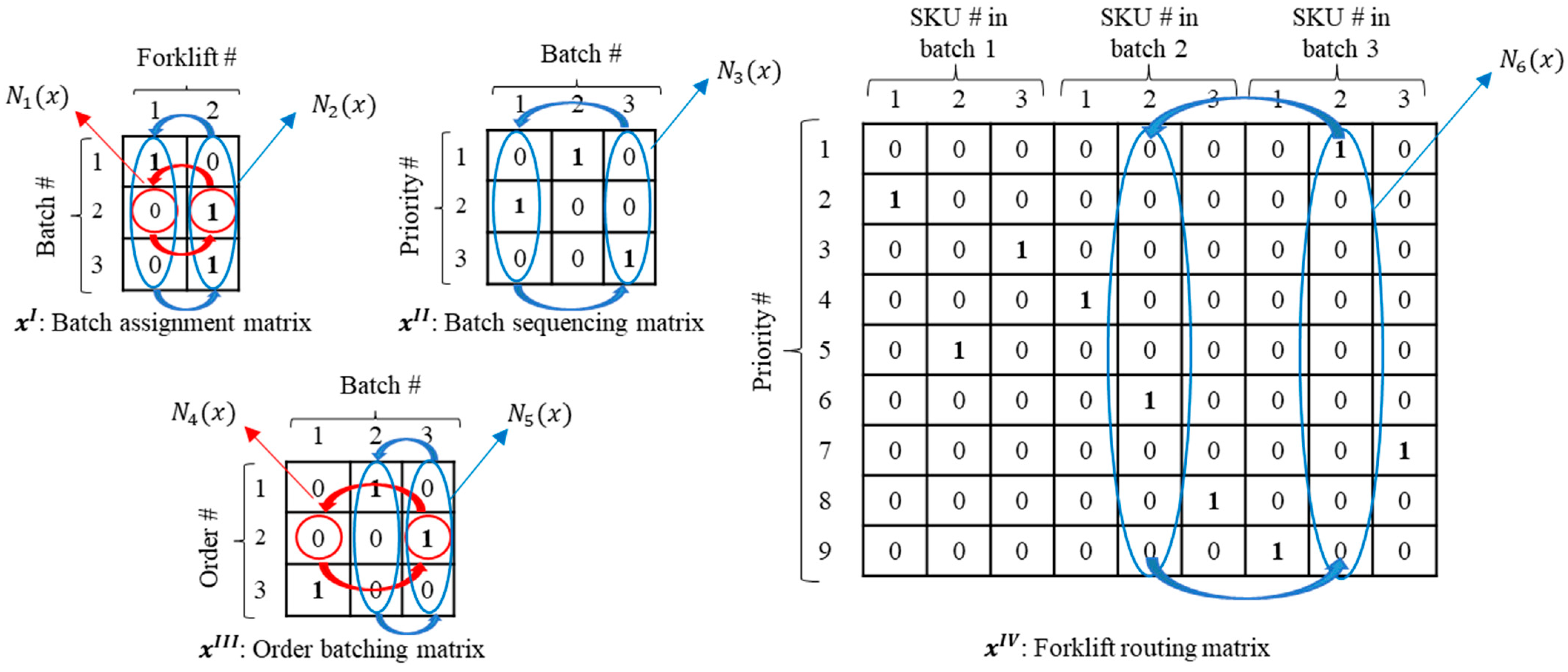
For all MOEAs, we use the same binary solution representation $x$ consisting of four decision matrices: (i) batch assignment, (ii) batch sequencing, (iii) order batching, and (iv) forklift routing. First, the batch assignment matrix is represented by $x^I\left(b,f\right)$, where $b\in \{1,\dots , B\}$ is the batch index, and $f\in \{1,\dots , F\}$ is the forklift index. Batch $b$ is assigned to forklift$f$ if $x^I\left(b,f\right)=1$(otherwise, $x^I\left(b,f\right)=0)$. Second, $x^{II}\left(p,b\right)$ denotes the batch sequencing matrix, where the row number $p\in \{1,\dots , B\}$ is the priority, and column $b\in \{1,\dots , B\}$ is the batch number. If $x^{II}\left(p,b\right)=1$, batch $b$ is prioritized as $p$^th batch (otherwise, $x^{II}\left(p,b\right)=0$). Third, the order batching matrix $x^{III}\left(o,b\right)$ is designed to assign only one batch $b\in \{1,\dots , B\}$ to each order $o\in \{1,\dots , O\}$. Batch $b$ is allocated to order $o$ if $x^{III}\left(o,b\right)=1$ (otherwise, $x^{III}\left(o,b\right)=0$). Last, matrix $x^{IV}\left(i,j\right)$ determines the sequence of forklift movements among $G$ SKUs/depots (SKU # $\in \left\{1,\dots , N\right\}$ and depot # $\in \{N+1,\dots , G\}$) in each batch $b\in \{1,\dots , B\}$.

Six neighborhood structures are designed to find neighborhood solutions for all MOEAs. $N_k(x)$ represents $k$^th neighborhood of solution $x$, where $k\in \{1,\dots , 6\}$. According to the solution representation, six neighborhood structures of solution $x$ can be defined with an example in Figure 2 and

Table 2. Information on illustrative examples for solution representation.

	Batch Assignment and Batch Sequencing			Order Batching				Forklift Routing among SKUs
Forklift No.	1	2	Batch No.	1	2	3	Forklift No.	1	2
Batch No.	1	2, 3	Order No.	3	1	2	SKU No.	Batch 1: 1, 3, 2	Batch 2: 1, 2, 3 Batch 3: 2, 3, 1

. $N_1(x)$ and $N_2(x)$ are associated with batch assignment matrix$x^I$. $N_1(x)$ randomly selects one row and two columns of $x^I$ so that the crossing elements are swapped. In other words, only one batch may be assigned to a new forklift with $N_1(x)$. $N_2(x)$ swaps two random columns in $x^I$; thus, the entire batches that are assigned to two different forklifts may be swapped with $N_2(x)$. For the batch sequencing matrix $x^{II}$, the neighborhood structure $N_3(x)$ is defined to change the sequence of two batches by swapping two random columns of $x^{II}$. $N_4(x)$ and $N_5(x)$ are designed to find a neighborhood solution based on the information on the order batching matrix $x^{III}$. $N_4(x)$ swaps two matrix elements which are chosen by one random row and two random columns from $x^{III}$. Only one order may switch from one batch to another in $N_4(x)$. In addition, $N_5(x)$ exchanges all orders between two batches by swapping two columns of $x^{III}$, randomly. Finally, $N_6(x)$ mutually changes the information in two random columns from the forklift routing matrix $x^{IV}$ to change the priority of two SKUs that should be picked up by forklifts.

3.2. MOEA Operators

The Pareto-optimal front (or frontier) is the set of all Pareto-optimal solutions found. Multi-objective methodologies provide a set of optimal solutions in the form of a Pareto-optimal front or frontier, instead of a single optimal solution. No solution is better than another among the solutions on a Pareto-optimal frontier. In other words, Pareto-optimal solutions are not dominated by any other solution. The strategy of MOEAs is to maintain both accuracy and diversity in obtaining the Pareto-optimal solutions by applying different effective operators. In this study, we improve and use five operators of NSGA-II [37]: (i) fast non-dominated sorting (FNS), (ii) crowding distance measurement (CDM), (iii) solution comparison and sorting (SCS), (vi) genetic crossover (GC), and (v) genetic mutation (GM) [37]. FNS is for sorting all solutions found as non-dominated frontier sets on different non-domination levels. For example, the solutions on the first non-dominated front are Pareto-optimal solutions, and the solutions on the second non-dominated front become Pareto-optimal solutions if the first front solutions are excluded or removed. CDM is the estimated density of the solutions: it is the average perimeter of a cuboid formed using nearest neighbor solutions as vertices. SCS is used for comparing the solutions by using rank and distance solution information. GC is used for exchanging some parts of the solution with another solution in solution representations and is for mixing the solutions and convergence in a subspace. GM is for changing randomly selected parts of one solution to improve the diversity of the population. Algorithms 1–5 introduces the pseudocodes of these five operators.

Algorithm 1. Pseudocode of FNS.

1.  $\mathbf{Input}\mathbf{:} \mathrm{Solutions} x_i$ $\in$ population $P$ 2.  Output: Pareto fronts $F_g$ and ${rank}_{x_i}$ for $x_i\in P$  % ${rank}_{x_i}$ is the non-domination rank of $x_i\in P$ 3.  for $x_i\in P$ do 4.    ${rank}_{x_i}≔$0 5.  end for 6.  $g≔1$         % Front counter 7.  while $\sum _g\left|F_g\right|<\left|P\right|$     % $\left|F_g\right|$ and $\left|P\right|$ are the front size and population size, respectively 8.    $F_g≔\varnothing$ 9.    for $x_i\in P$ do 10.     if ${rank}_i≔$0 then 11.       for $x_{j\ne i}\in P$ do 12.         if $x_i\prec x_j$ then   % If $x_i$ dominates $x_j$ 13.           $F_g≔F_g\cup \left\{x_i\right\}$ 14.           ${rank}_{x_i}≔g$ 15.         else 16.           $F_g≔F_g\backslash \left\{x_i\right\}$ 17.           ${rank}_{x_i}≔0$ 18.         end if 19.       end for 20.     end if 21.   end for 22.   $g≔g+1$ 23. end while

Algorithm 2. Pseudocode of CDM.

1.  $\mathbf{Input}\mathbf{:} \mathrm{Pareto} \mathrm{front} F$ and objective functions $f_{k\in \{1,\dots , K\}}(x_i)$ for $x_i\in F$ 2.  Output: ${distance}_{x_i}$ for $x_i\in F$   % ${distance}_{x_i}$ is the crowding distance of $x_i\in F$ 3.  for $x_i\in F$ do 4.    ${distance}_{x_i}≔0$ 5.  end for 6.  for   $k\in \{1,\dots , K\}$ do 7.    $F≔$sort ($F$)     % Sort $x_i\in F$ from the worst $f_k(x_i)$ or ${f_{}}_k^{max}$ to the best $f_k(x_i)$or ${f_{}}_k^{min}$ 8.    ${distance}_{F(1)}≔\infty$    %$F(1)$ is the first solution of $F$ 9.    ${distance}_{F(|F|)}≔\infty$   % $F(|F|)$ is the last solution of $F$, where $\left|F\right|$ is the font size 10.   for $i=2$ to ($\left|F\right|-1$) 11.     ${distance}_{F\left(i\right)}≔{distance}_{F\left(i\right)}+\frac{{distance}_{F\left(i+1\right)}-{distance}_{F\left(i-1\right)}}{{f_{}}_k^{max}-{f_{}}_k^{min}}$ 12.   end for 13. end for

Algorithm 3. Pseudocode of SCS.

Input: ${rank}_{x_i}$, ${rank}_{x_j}$, ${distance}_{x_i}$, and ${distance}_{x_j}$ Output: $x_i{\prec }_n{x}_j$ or $x_j{\prec }_n{x}_i$ if ${rank}_{x_i}<{rank}_{x_j}$then   $x_i{\prec }_n{x}_j$  else if  ${rank}_{x_i}={rank}_{x_j}$ and ${distance}_{x_i}>{distance}_{x_j}$ then   $x_i{\prec }_n{x}_j$ else   $x_j{\prec }_n{x}_i$ end if

Algorithm 4. Pseudocode of GC.

1.  Input: Solution matrices of parent 1 ($x_{ p1}^I$, $x_{ p1}^{II}$,$x_{ p1}^{III}$, and $x_{ p1}^{IV}$) and parent 2 ($x_{ p2}^I$, $x_{ p2}^{II}$,$x_{ p2}^{III}$, and $x_{ p2}^{IV}$) 2.  Output: Solution matrices of offspring 1 ($x_{ off1}^I$, $x_{ off1}^{II}$,$x_{ off1}^{III}$, and $x_{ off1}^{IV}$) and offspring 2 ($x_{ off2}^I$, $x_{ off2}^{II}$,$x_{ off2}^{III}$, and $x_{ off2}^{IV}$) 3.  $r^I≔$ Random column from $x^I$ 4.  $x_{ off1}^I(:, 1:r^I)≔x_{ p1}^I(:, 1:r^I)$ 5.  $x_{ off1}^I(:,r^I+1:F)≔x_{ p2}^I(:, r^I+1:F)$  % $F$ is the number of forklifts. 6.  $x_{ off2}^I(:, 1:r^I)≔x_{ p2}^I(:, 1:r^I)$ 7.  $x_{ off2}^I(:,r^I+1:F)≔x_{ p1}^I(:, r^I+1:F)$   % $F$ is the number of forklifts. 8.  $r^{II}≔$ Random column from $x^{II}$ 9.  $x_{ off1}^{II}(:, 1:r^{II})≔x_{ p1}^{II}(:, 1:r^{II})$ 10. $x_{ off1}^{II}(:,r^{II}+1:B)≔x_{ p2}^{II}(:, r^{II}+1:B)$   % $B$ is the number of batches. 11. $x_{ off2}^{II}(:, 1:r^{II})≔x_{ p2}^{II}(:, 1:r^{II})$ 12. $x_{ off2}^{II}(:,r^{II}+1:B)≔x_{ p1}^{II}(:, r^{II}+1:B)$   % $B$ is the number of batches. 13. $r^{III}≔$ Random column from $x^{III}$ 14. $x_{ off1}^{III}(:, 1:r^{III})≔x_{ p1}^{III}(:, 1:r^{III})$ 15. $x_{ off1}^{III}(:,r^{III}+1:B)≔x_{ p2}^{III}(:, r^{III}+1:B)$  % $B$ is the number of batches. 16. $x_{ off2}^{III}(:, 1:r^{III})≔x_{ p2}^{III}(:, 1:r^{III})$ 17. $x_{ off2}^{III}(:,r^{III}+1:B)≔x_{ p1}^{III}(:, r^{III}+1:B)$  % $B$ is the number of batches. 18. $r^{IV}≔$ Random column from $x^{IV}$ 19. $x_{ off1}^{IV}(:, 1:r^{IV})≔x_{ p1}^{IV}(:, 1:r^{IV})$ 20. $x_{ off1}^{IV}(:,r^{IV}+1:B·G)≔x_{ p2}^{IV}(:, r^{IV}+1:B·G)$  % $B$ and $G$ are the number of batches and SKUs/depots, respectively. 21. $x_{ off2}^{IV}(:, 1:r^{IV})≔x_{ p2}^{IV}(:, 1:r^{IV})$ 22. $x_{ off2}^{IV}(:,r^{IV}+1:B·G)≔x_{ p1}^{IV}(:, r^{IV}+1:B·G)$  % $B$ and $G$ are the number of batches and SKUs/depots, respectively.

Algorithm 5. Pseudocode of GM.

Input: Incumbent solution $x$ Output: Neighbor solution $x^{\prime }$ Randomly select a neighborhood structure $N_k\left(x\right),$where $k\in \{1,\dots ,6\}$ $x^{\prime }≔$ Random solution generated from the $k$th neighborhood of $x$ ($x^{\prime }\in N_k\left(x\right)$)

In addition to the five operators above, we design a new operator, multi-objective variable neighborhood search (MOVNS) based on the single-objective variable neighborhood search (VNS) [38]. The operator enables the NSVNS, NSGA-VNS, and NSGS-VNS-DLS proposed in this study to find local optimum solutions; MOVNS helps these new algorithms maintain diversity in finding solutions by applying multiple neighborhood structures instead of one. MOVNS executes a sequence of local searches for solution $x$ using the six neighborhood structures $N_{k\in \{1,\dots ,6\}}(x)$ presented in Section 3.1. Algorithm 6 exhibits the pseudocode of the MOVNS operator.

Algorithm 6. Pseudocode of MOVNS.

1.  Input: Incumbent solution $x$and number of searches in each neighborhood structure $NS$ 2.  Output: $x"$ 3.  %Shaking: 4.  $S≔\varnothing$ 5.  Randomly select an initial neighborhood structure $N_{initial}\left(x\right),$where $initial\in \{1,\dots ,6\}$ 6.  for $i\in \left\{1,\dots ,NS\right\}$ do 7.    $x^{\prime }≔$ Random solution generated from the $k$th neighborhood of $x^{\prime }$ ($x^{\prime }\in N_{initial}\left(x\right)$) 8.    $S≔S\cup \left\{x^{\prime }\right\}$ 9. end for 10. $x^{\prime }≔$ Non-dominated solution found from $S$ 11. % Local search: 12. $S≔\varnothing$ 13. for $k\in \left\{1,\dots ,6\right\}\backslash \left\{initial\right\}$ do 14.   for $i\in \left\{1,\dots ,NS\right\}$ do 15.     $x"≔$ Random solution generated from the $k$th neighborhood of $x^{\prime }$ ($x"\in N_{initial}(x\prime )$) 16.     $S≔S\cup \{x"\}$ 17.   end for 18. end for 19. $x"≔$ Non-dominated solution found from $S$

3.3. New MOEA-1: NSVNS

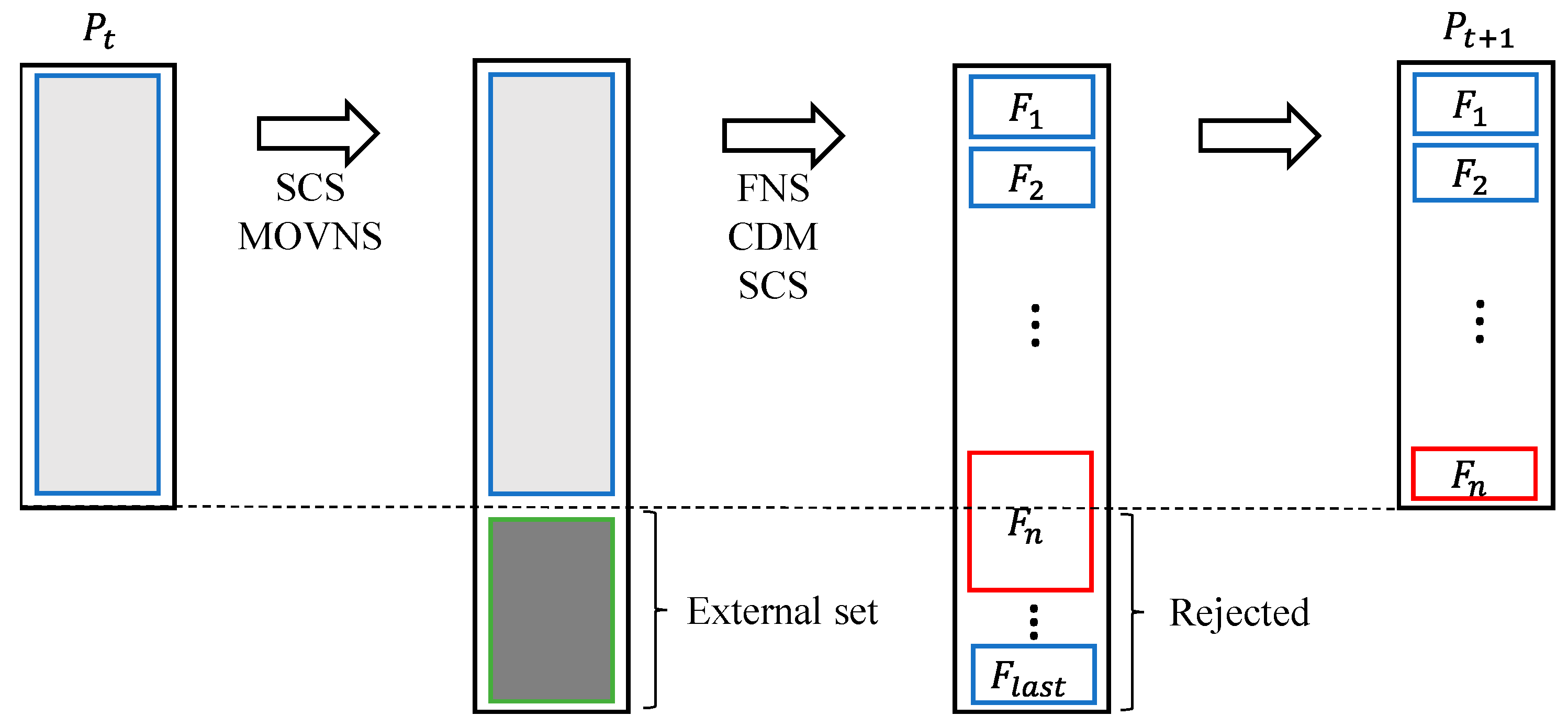
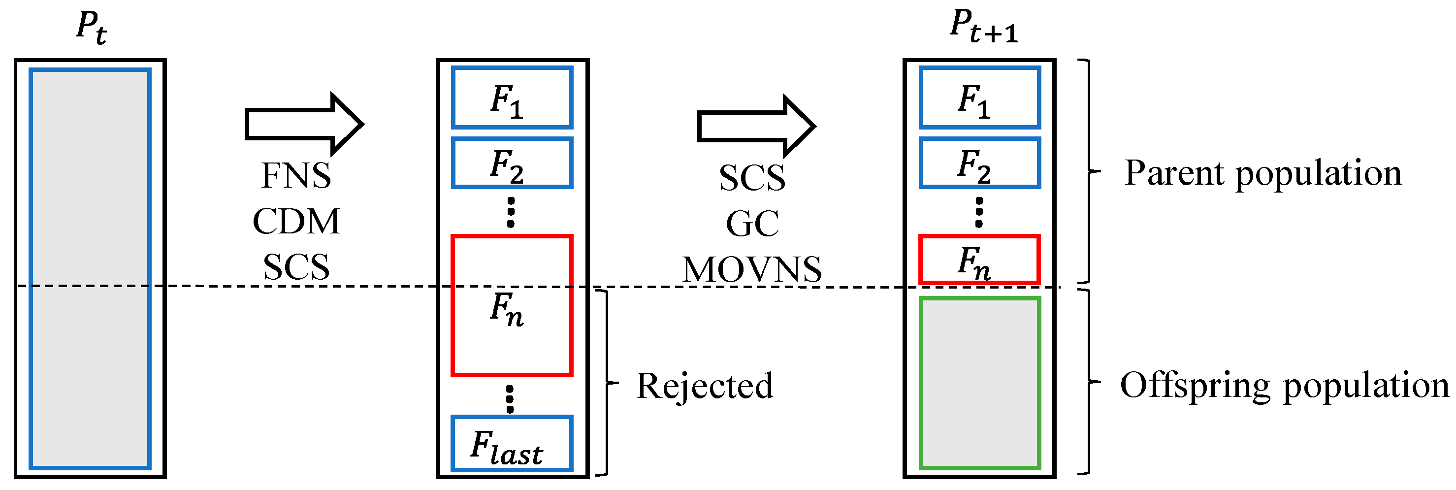
Non-dominated sorting variable neighborhood search (NSVNS) applies fast and elitist operators, FNS, CDM, SCS, and MOVNS, to find a Pareto-optimal front in solving problems. NSVNS also uses an external set consisting of the best neighbors in the population. This algorithm first picks solution candidates from the population using an SCS-based tournament selection in Algorithm 3. Then, the MOVNS operator is executed for each candidate solution to build the external set in Algorithm 6. The external set integrates with the original population to reach a new population with more neighborhood information. NSVNS can find diverse solutions with this dynamic population. In the next step, NSVNS sorts the solutions of the population on different fronts with different ranks using the FNS operator in Algorithm 1. In addition, the CDM operator is applied to calculate the crowding distance value of each solution located on the same front. From the results of FNS and CDM, the SCS operator is again applied to sort the entire population. Finally, extra solutions are removed to return to the original population size. The mechanism and pseudocode of NSVNS are presented in Figure 3 and Algorithm 7.

Algorithm 7. Pseudocode of NSVNS.

1.  Input: Population size $\left|P\right|$, external set size $\left|ES\right|$, number of searches in each neighborhood structure $NS$, and maximum iteration number $t_{max}$ (stopping criterion) 2.  Output: Pareto-optimal front 3.  Randomly generate an initial population $P_1$ 4.  Execute Algorithm 1 for $P_1$    % FNS operator 5.  Execute Algorithm 2 for $P_1$    % CDM operator 6.  Execute Algorithm 3 for $P_1$    % SCS operator 7.  for $t\in \left\{1,\dots ,t_{max}\right\}$ do 8.    $ES≔\varnothing$ 9.    for $i\in \left\{1,\dots ,\left|ES\right|\right\}$ do 10.     Execute an SCS-based tournament selection to pick one candidate solution $x$ from $P_t\left(1:\left|P\right|\right)$ 11.     Execute Algorithm 6 for $x$  % MOVNS operator 12.     $ES≔EC\cup \left\{x\right\}$ 13.   end for 14.   $P_t≔P_t\cup EC$ 15.   Execute Algorithm 1 for $P_t$  % FNS operator 16.   Execute Algorithm 2 for $P_t$  % CDM operator 17.   Execute Algorithm 3 for $P_t$  % SCS operator 18.   $P_t≔P_t\left(1:\left|P\right|\right)$ 19. end for

3.4. New MOEA-2: NSGA-MOVNS

The structure of NSGA-II and MOVNS (NSGA-MOVNS) is similar with a difference in the mutation operator. Both algorithms begin with a random initial population. At each iteration/generation, the solutions of the population are categorized into different Pareto fronts with different ranks by using a sorting operator (FNS) in Algorithm 1. When the solutions are assigned to different Pareto fronts, the crowding distance value of each solution is measured using the CDM operator in Algorithm 2. Then, the population is sorted, and a specific number of solutions are selected to remain for the next generation using the SCS operator based on Algorithm 3. Some of the remaining solutions are chosen as parents using an SCS-based tournament selection to generate the offspring of the generation and complete the population. The selected parents are combined using the GC operator in Algorithm 4. In addition, the offspring may mutate based on the probability of finding local solutions. NSGA-II uses only a single neighborhood structure for the offspring’s mutations such as the GM operator in Algorithm 5; instead, offspring mutate based on multiple neighborhood structures in NSGA-MOVNS using the MOVNS operator in Algorithm 6. The mechanism of NSGA-MOVNS is shown in Figure 4. In addition, Algorithm 8 provides the details of NSGA-MOVNS.

Algorithm 8. Pseudocode of NSGA-MOVNS.

1.  Input: Population size $\left|P\right|$, parent population size $\left|par\right|=\left|par\right| ·$crossover probability $p_m$, maximum iteration number $t_{max}$ (stopping criterion), mutation probability $p_m$, and the number of searches in each neighborhood structure $NS·$ 2.  Output: Pareto-optimal front 3.  Randomly generate an initial population $P_1$ 4.  for $t\in \left\{1,\dots ,t_{max}\right\}$ do 5.    Execute Algorithm 1 for $P_t$   % FNS operator 6.    Execute Algorithm 2 for $P_t$   % CDM operator 7.    Execute Algorithm 3 for $P_t$   % SCS operator 8.    $P_{t+1}\left(1:\left|par\right|\right)≔P_t\left(1:\left|par\right|\right)$ 9.    for $i\in \left\{1,\dots ,\frac{\left|P\right|-\left|par\right|}{2}\right\}$ do 10.     Execute an SCS-based tournament selection to pick two parents from $P_t\left(1:\left|par\right|\right)$ 11.     Execute Algorithm 4 (GC operator) to generate two offspring $x_{off1}$ and $x_{off2}$ 12.     $r≔R$andom number from the uniform distribution U [0, 1] 13.     if $r<p_m$ then 14.       Execute Algorithm 6 for $x_{off1}$   % MOVNS operator 15.     end if 16.     $r≔R$andom number from the uniform distribution U [0, 1] 17.     if  $r<p_m$ then 18.       Execute Algorithm 6 for $x_{off2}$  % MOVNS operator 19.     end if 20.     $P_{t+1}≔P_{t+1}\cup \left\{x_{off1}\right\}$ 21.     $P_{t+1}≔P_{t+1}\cup \left\{x_{off2}\right\}$ 22.   end for 23. end for

3.5. New MOEA-3: NSGA-VNS-DLS

NSGA-II and NSVNS with a dynamic learning strategy (NSGA-VNS-DLS) are designed to balance the advantages of both NSGA-II and NSVNS by achieving an accurate and diverse Pareto-optimal front [26]. The dynamic mechanism of NSGA-VNS-DLS uses a probability rule $p\in [0, 1]$ which is calculated based on the incumbent iteration number $t$ and the maximum iteration number $t_{max}$ of the algorithm ($p=\frac{t}{t_{max}}$). NSGA-VNS-DLS therefore gradually switches from NSGA-II to NSVNS as $p\to 1,$ as shown by Algorithm 9.

Algorithm 9. Pseudocode of NSGA-VNS-DLS.

1.  Input: Population size $\left|P\right|$, parent population size $\left|par\right|$, external set size $\left|ES\right|$, maximum iteration number $t_{max}$ (stopping criterion), mutation probability $p_m$, and the number of searches in each neighborhood structure $NS$ 2.  Output: Pareto-optimal front 3.  Randomly generate an initial population $P_1$ 4.  Execute Algorithm 1 for $P_1$  % FNS operator 5.  Execute Algorithm 2 for $P_1$  % CDM operator 6.  Execute Algorithm 3 for $P_1$  % SCS operator 7.  for $t\in \left\{1,\dots ,t_{max}\right\}$ do 8.    $r≔R$andom number from the uniform distribution U [0, 1] 9.    if $r<\frac{t}{t_{max}}$ then 10.     % Main loop of NSGA-II 11.     Execute the main loop of Algorithm 8 (NSGA-MOVNS) in which Algorithm 6 (MOVNS) is replaced with Algorithm 5 (GM) 12.   else 13.     %Main loop of NSVNS 14.     Execute the main loop of Algorithm 7 15.   end if 16. end for

3.6. Parameter Tuning of MOEAs

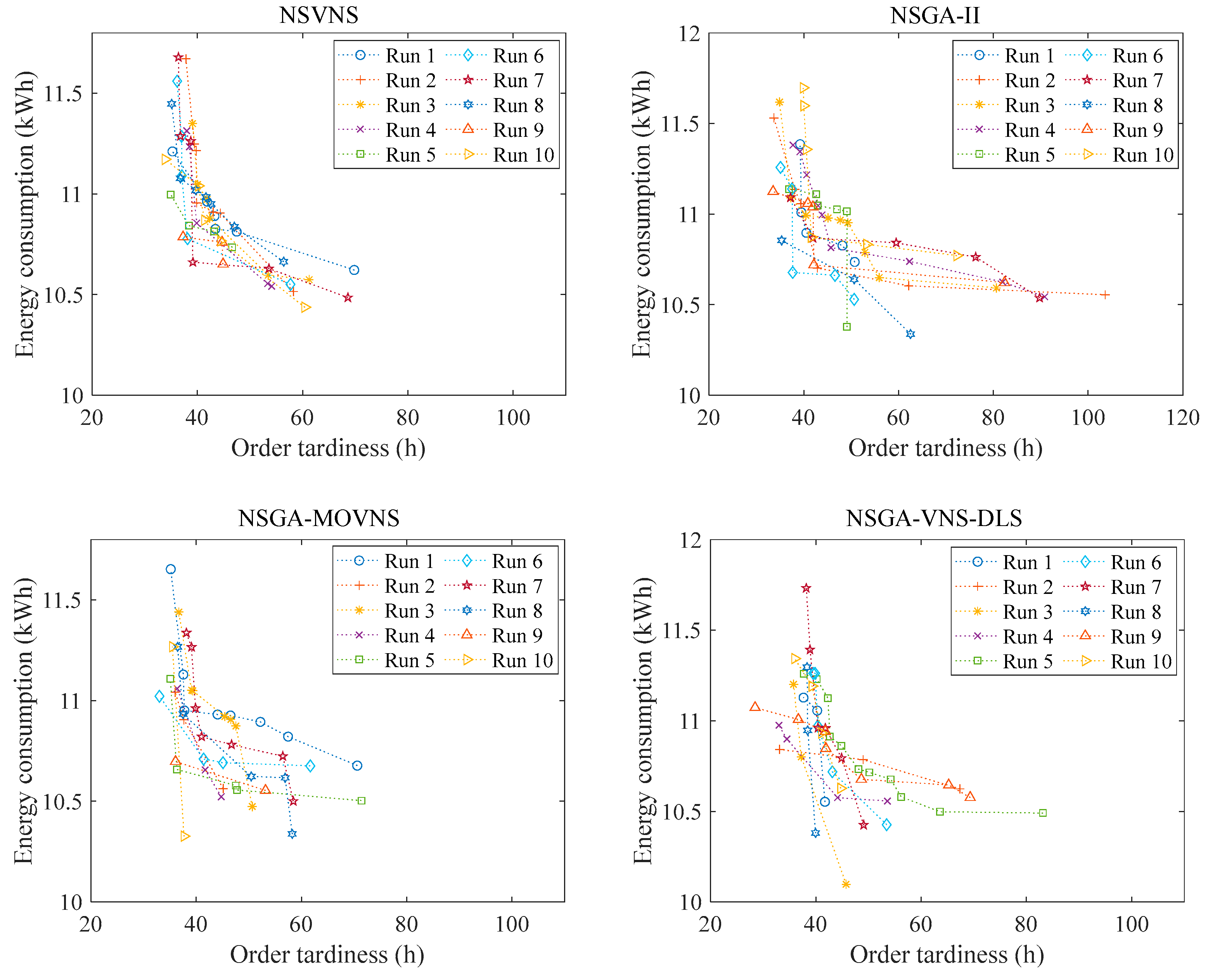
The parameters of MOEAs need to be tuned to guarantee the algorithms’ robustness when compared to each other. To calibrate the parameters of MOEAs, we use the Taguchi experimental design presented by [39] with Minitab 19. The Taguchi design categorizes the parameters into controllable parameters and noise parameters. While a control parameter can be controlled over the process, a noise parameter is uncontrollable and can only be handled during experimentation. Different levels of the experiment need to be defined for each parameter, and a single-to-noise (S/N) ratio is calculated for each combination of the control parameters represented as orthogonal arrays. The average S/N ratio is also measured for each level of each control parameter. The Taguchi design uses the S/N ratio to adjust the control parameters to reduce the variability caused by noise parameters. A higher S/N ratio implies a better experimental level of a control parameter compared to the effects of the noise parameters. Since the goal of this experiment is to minimize a response, we use an S/N ratio formulation known as “smaller-is-better” as $S/N=-10·\mathit{log}(\frac{\sum Y^2}{n})$, where n is the combination of the control parameters, and Y is the response variable [40,41]. In this study, we examine the variability of the response $Y=\frac{MMID}{DM}$, where modified mean ideal distance (MMID), and diversity metric (DM) are the modified mean ideal distance and the diversity metrics, respectively [42,43]. For MMID, smaller values are preferred, and for DM, larger values are preferred. In the Taguchi experimental design, we use the best Pareto-optimal frontiers in terms of $\frac{MMID}{DM}$ obtained from 10 runs of each MOEA for a medium-sized case study with 100 orders, 5 SKUs each, and 5 forklifts, as shown in Figure 5.

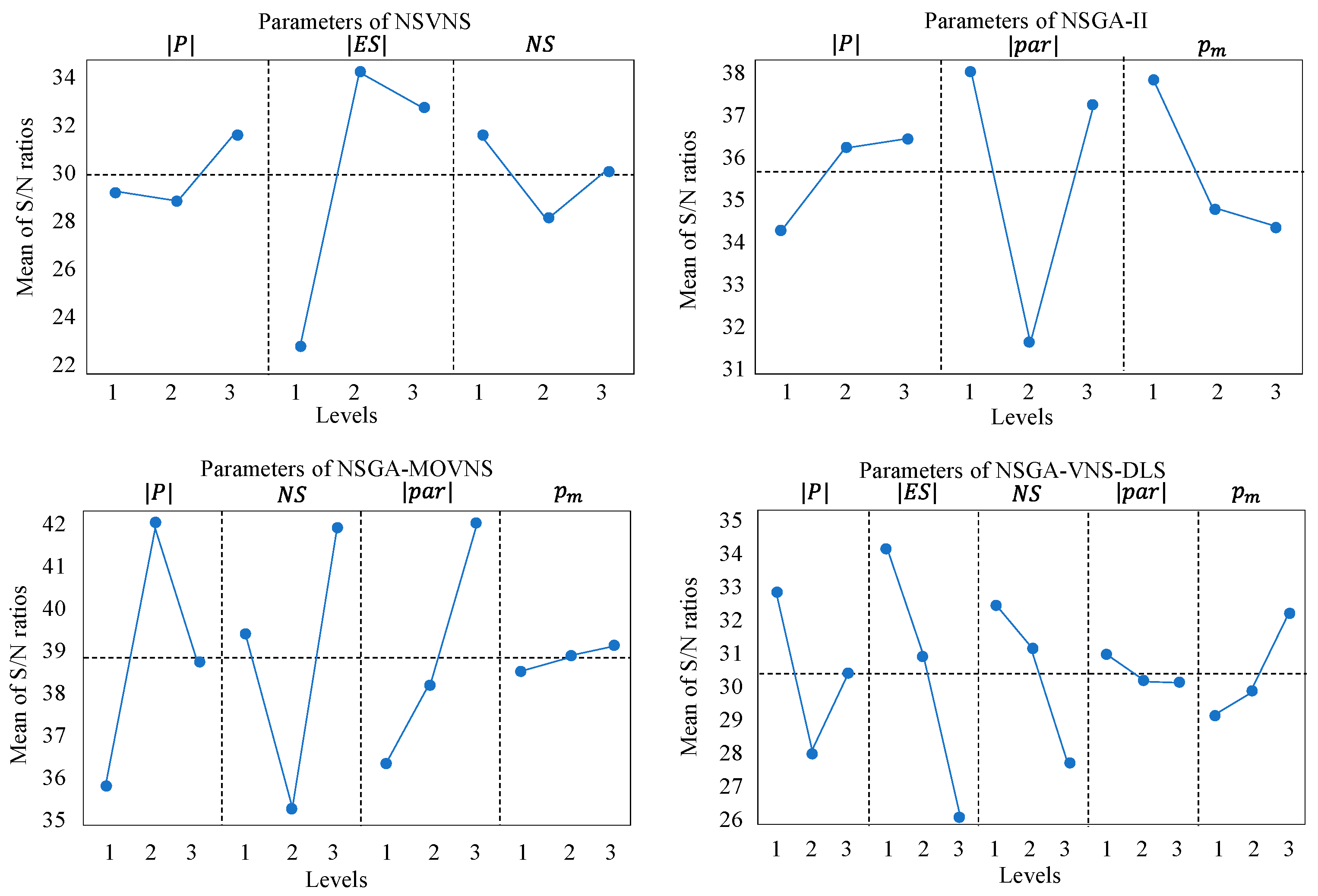
While we assume the same maximum iteration number $t_{max}=1000$ (stopping criterion) for all algorithms, we design the Taguchi experiment for all other parameters of MOEA with three levels, as shown in

Table 3. Parameter tuning of MOEAs using Taguchi method.

Parameters	Levels	Values	Algorithms
			NSVNS	NSGA-II	NSGA-MOVNS	NSGA-VNS-DLS
$\left|P\right|$	1	50				✔
	2	100			✔
	3	200	✔	✔
$\left|ES\right|$	1	$⌊0.1·\left|P\right|⌋$		N/A	N/A	✔
	2	$⌊0.3·\left|P\right|⌋$	✔	N/A	N/A
	3	$⌊0.5·\left|P\right|⌋$		N/A	N/A
$NS$	1	2	✔	N/A		✔
	2	3		N/A
	3	4		N/A	✔
$\left|par\right|$	1	$⌊0.7·\left|P\right|⌋$	N/A	✔		✔
	2	$⌊0.8·\left|P\right|⌋$	N/A
	3	$⌊0.9·\left|P\right|⌋$	N/A		✔
$p_m$	1	0.1	N/A	✔
	2	0.2	N/A
	3	0.3	N/A		✔	✔

. The parameters of this experiment include population size $\left|P\right|$, parent population size $\left|par\right|$, external set size $\left|ES\right|$, mutation probability $p_m$, and number of searches in each neighborhood structure $NS$. The results of the Taguchi experiment suggest that $\left|ES\right|$ significantly affects the response for NSVNS and NSGA-VNS-DLS at a significance level of 0.05 (p-value < 0.05). Furthermore, we found a significant interaction between $NS$ and $p_m$ for NSGA-MOVNS (p-value < 0.05). No other significant parameters or interactions are found for MOEAs. The main effects plot of S/N ratios for all MOEAs is also presented in Figure 6. The maximum value of the S/N ratio is the criterion to select the best level of a parameter. Accordingly, Table 3 reports the tuned parameters with checkmarks.

4. Numerical Experiments

We present and solve 12 case studies in different sizes to verify the mathematical model in Section 2 and evaluate the performance of the MOEAs in Section 3. The relationship between EC and OT on Pareto-optimal frontiers (solutions) is also assessed with some managerial insights. In addition, the effects of important parameters of the problem on EC and OT are discussed.

4.1. Problem Parameters

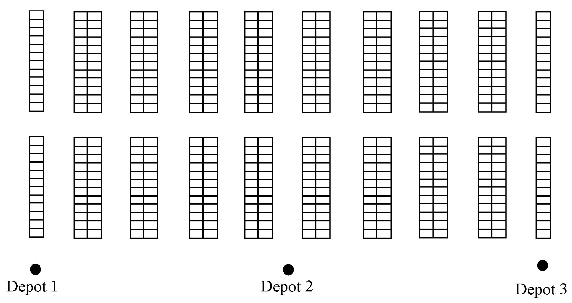
In our case studies, up to 30 SKU types are randomly selected to be picked from 1296 storage locations. In addition, a total of three depots are assumed; they are located at a ten-meter distance from the picking aisles. Figure 7 illustrates a bird’s eye view from the layout of the picker-to-parts system. In addition, the layout specifications of the designed picker-to-parts system are listed in

Table 4. Layout specifications of picker-to-parts system.

Layout Information	Specification
Number of storage locations	1296
Number of depots	3
Number of bays per rack	12
Number of tiers per rack	3
Number of racks	18
Number of aisles	18
Length	74 m
Width	48 m
Height	5 m
Length of rack	22 m
Width of rack	2 m
Height of rack	5 m
Length of aisle	22 m
Width of Aisle	5 m

. We consider 5, 10, 15, 25, 100, and 200 orders in the case studies. In addition, the number of SKUs (order size) is assumed to be 3, 5, or 10 [16,18]. The mass of each SKU ($m_i$) is randomly generated from the uniform distribution U [5, 50] in kg. Moreover, the due date of each order ($d_o$) is randomly chosen from $U\left[\alpha ,\frac{2·\left(1-\gamma \right)· \tilde{\alpha }+\alpha }{\beta }\right],$where $\alpha =7$ is the minimum order picking time in minute,$\tilde{\alpha }$ is the summation of order picking times, $\beta$ is the number of available forklifts, and $\gamma =0.6$ is modified traffic congestion which represents the due date tightness [16,44]. We assume three, five, and eight homogenous forklifts for the case studies. Each forklift is capable of picking a maximum of 45 SKUs ($C^f=45)$ with similar dimensions in each tour [16]. In addition, the mass capacity of forklifts is considered as 1360 kg. The average time of a battery’s fast charging ($\theta$) is assumed to be 20 min [45]. We collected real power data for 20 min from a charger of a lead-acid battery with 38 V, 1105 Ah, and 18 cells. Accordingly, we assume that the maximum EC of the forklift between two consecutive fast chargings $({EC}_{max}$) is 3.73 kWh.

EC of an electric forklift is the amount of power used over its travel time. The operating factors of the forklift such as A/D and velocity are important for modeling the travel time. Following the travel time model proposed by [46], we study the relationships between the forklift A/D, velocity, and travel time. Afterward, we estimate electric-forklift EC based on real power data of a forklift with approximately 5971 kg weight given by a forklift manufacturer [36]. Two scenarios can occur when a forklift travels in the horizontal direction $x$ or vertical direction $y$. In Figure 8, the forklift in the first scenario cannot travel as far as the travel distance ($d_{peak}$), which is needed to reach $v_{max}$, while it reaches the maximum velocity $v_{max}$ in the second scenario. In this study, we assume only the horizontal and vertical movements of a forklift traveling from SKU $i$ to another SKU $j$. Therefore, the general relationships defined between the forklift A/D, velocity, and travel time through the two travel scenarios can be applied to both horizontal and vertical directions. Figure 9 illustrates the four possible combinations with movement directions.

Figure 10 shows the power and velocity of an electric forklift in the time resolution of 0.01 s for the forklift’s horizontal and vertical movements, respectively [36]. According to the data, the forklift applies the average A/D of $a^x=0.409$ m/s² for 8.73 s and remains at the maximum constant velocity of $v_{max}^x=3.576$ m/s from 8.74 to 15.41 s in the horizontal direction $x$. Therefore, we calculate travel time $t_{i,j}^x$ in the horizontal direction $x$ by Equation (25) based on $a^x$, $v_{max}^x$, and the distance between SKUs i and j ($d_{i,j}^x$). Equation (26) measures travel time $t_{i,j}^y$ in the vertical direction $y$ according to $d_{i,j}^y$, $t_v=4.97$ s, and the two vertical constant velocities are $v_1^y=1.162$ m/s (0 to 4.97 s) and $v_2^y=0.76$ m/s (4.97 to 6.8 s). The data implies that the forklift is designed with regenerative braking that can charge the batteries. This study assumes that the forklift can immediately stop without any deceleration or braking time.

$$t_{i,j}^x=\left\{\begin{array}{c}\sqrt{\frac{4·d_{i,j}^x}{a^x}} 0\le d_{i,j}^x\le d_{peak}^x\\ \frac{d_{i,j}^x}{v_{max}^x}+\frac{v_{max}^x}{a^x} d_{peak}^x\le d_{i,j}^x \end{array}\right.$$

(25)

$$t_{i,j}^y=\left\{\begin{array}{c}\frac{d_{i,j}^y}{v_1^y} 0\le d_{i,j}^y\le v_1^y{·t}_v\hfill \\ t_v+\frac{d_{i,j}^y-v_1^y{·t}_v}{v_2^y} v_1^y{·t}_v\le d_{i,j}^y \hfill \end{array}\right.$$

(26)

4.2. Validation and Comparison of Algorithms

To validate and solve multi-objective problems proposed in Section 2, AUGMECON (exact solution method) is applied for 12 case studies [27]; all constraints and equations of the mathematical model presented in Section 2 are checked to be satisfied and validated. AUGMECON could solve three small examples (Cases 1–3), but no answer is obtained within a 20 h run for medium- to large-sized case studies, using the Gurobi 9 solver in Python. AUGMECON finds the Pareto-optimal solutions for Cases 1, 2, and 3 on the average of 32,191 s whereas NSVNS (44 s), NSGA-II (39 s), NSGA-MOVNS (143 s), and NSGA-VNS-DLS (331 s) take significantly less time to solve the three problems. The Pareto-optimal solutions (frontiers) found by AUGMECON and MOEAs are listed in

Table 5. Pareto-optimal solutions by AUGMECON and MOEAs.

Case 1 (5 Orders, 3 SKUs Each, and 3 Forklifts)
		Algorithms
		AUGMECON		NSVNS		NSGA-II		NSGA-MOVNS		NSGA-VNS-DLS
Solutions		${\mathit{f}}_{\mathit{E}\mathit{C}}$	${\mathit{f}}_{\mathit{O}\mathit{T}}$	${\mathit{f}}_{\mathit{E}\mathit{C}}$	${\mathit{f}}_{\mathit{O}\mathit{T}}$	${\mathit{f}}_{\mathit{E}\mathit{C}}$	${\mathit{f}}_{\mathit{O}\mathit{T}}$	${\mathit{f}}_{\mathit{E}\mathit{C}}$	${\mathit{f}}_{\mathit{O}\mathit{T}}$	${\mathit{f}}_{\mathit{E}\mathit{C}}$	${\mathit{f}}_{\mathit{O}\mathit{T}}$
1		0.502	1.216	0.508	1.015	0.623	0.255	0.507	1.147	0.535	0.920
2		0.611	0.366			0.775	0.182	0.691	0.046	0.61	0.704
3		0.651	0.342							0.706	0.073
4		0.77	0.318
5		0.79	0.046
Case 2 (10 orders, 3 SKUs each, and 3 forklifts)
		Algorithms
		AUGMECON		NSVNS		NSGA-II		NSGA-MOVNS		NSGA-VNS-DLS
Solutions		${\mathit{f}}_{\mathit{E}\mathit{C}}$	${\mathit{f}}_{\mathit{O}\mathit{T}}$	${\mathit{f}}_{\mathit{E}\mathit{C}}$	${\mathit{f}}_{\mathit{O}\mathit{T}}$	${\mathit{f}}_{\mathit{E}\mathit{C}}$	${\mathit{f}}_{\mathit{O}\mathit{T}}$	${\mathit{f}}_{\mathit{E}\mathit{C}}$	${\mathit{f}}_{\mathit{O}\mathit{T}}$	${\mathit{f}}_{\mathit{E}\mathit{C}}$	${\mathit{f}}_{\mathit{O}\mathit{T}}$
1		0.962	3.748	0.974	1.85	1.009	3.124	1.007	0.84	0.993	1.775
2		1.068	0.6			1.118	0.338	1.114	0.384	1.032	1.75
3		1.214	0.207					1.099	0.408
Case 3 (15 orders, 3 SKUs each, and 3 forklifts)
		Algorithms
		AUGMECON		NSVNS		NSGA-II		NSGA-MOVNS		NSGA-VNS-DLS
Solutions		${\mathit{f}}_{\mathit{E}\mathit{C}}$	${\mathit{f}}_{\mathit{O}\mathit{T}}$	${\mathit{f}}_{\mathit{E}\mathit{C}}$	${\mathit{f}}_{\mathit{O}\mathit{T}}$	${\mathit{f}}_{\mathit{E}\mathit{C}}$	${\mathit{f}}_{\mathit{O}\mathit{T}}$	${\mathit{f}}_{\mathit{E}\mathit{C}}$	${\mathit{f}}_{\mathit{O}\mathit{T}}$	${\mathit{f}}_{\mathit{E}\mathit{C}}$	${\mathit{f}}_{\mathit{O}\mathit{T}}$
1		2.111	12.058	2.117	1.51	2.174	1.932	2.141	2.231	2.16	5.729
2		2.602	4.318					2.204	2.074	2.177	1.801
3		2.533	3.578					2.326	1.813	2.215	0.865
4		2.673	0.865

. In the table, the AUGMECON solutions are all solutions found by AUGMECON with one run. For the four MOEAs, the Pareto-optimal solutions are found with ten runs, but only solutions non-dominated by any AUGMECON solutions are reported. This clearly shows the limitation of the exact solution method (AUGMECON); it takes almost 10 times longer to run AUGMECON (32191 s) once than to run NSGA-VNS-DLS 10 times (331 × 10 s) while the number of solutions found is comparable between AUGMECON and MOEAs.

4.3. Performance Comparison of MOEAs

To evaluate the quality of non-dominated solutions obtained from MOEAs, we consider five metrics: (i) the number of Pareto-optimal solutions/frontiers (NPS), (ii) MMID, (iii) DM, (iv) spacing metric (SM), and (v) CPU time. NPS is the basic metric to show the number of Pareto-optimal frontiers each MOEA can provide. MMID is calculated based on the distances from non-dominated solutions to an ideal point [42], and lower MMID indicates a better convergence ability toward an ideal point. DM represents the spread of non-dominated solutions in the search domain and is the measurement of the Euclidean distance between the endpoints of Pareto-optimal solutions [43]. Higher DM indicates better Pareto-optimal solutions with more diversity. SM is the standard deviation of solution distances and is used to examine the consistency of distances between solutions [47]. Low SM indicates more distance consistency between the non-dominated solutions. CPU time is an important metric for evaluating the computational cost of each algorithm.

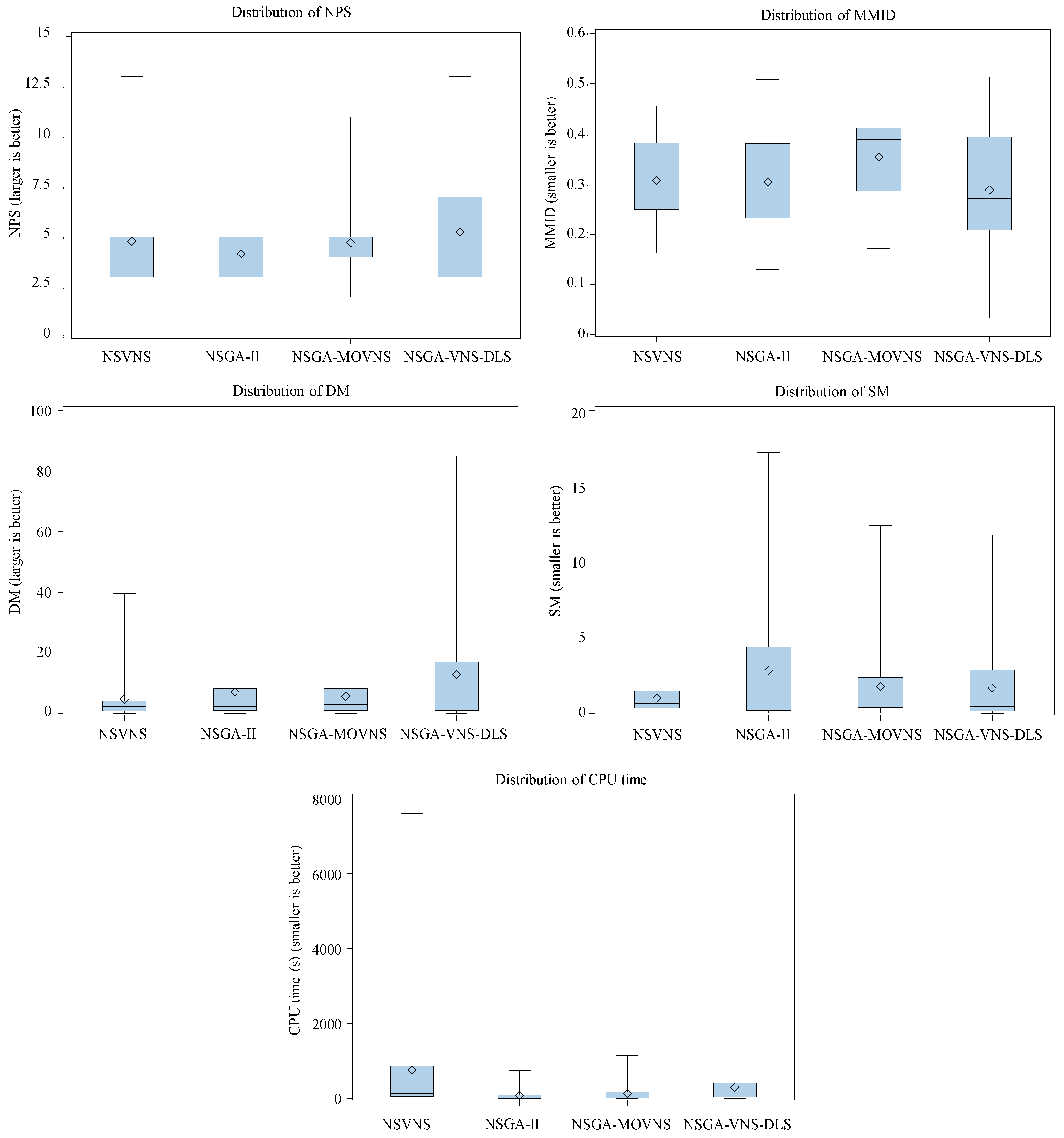
To compare the performances of MOEAs in terms of the metrics of NPS, MMID, DM, SM, and CPU time, we designed two types of experiments: completely randomized design (CRD) and randomized block design (RBD). Each MOEA with 1000 iterations is executed over 10 replications for all 12 case studies to construct CRD and RBD in SAS 9.4 software. We apply the one-way analysis of variance (ANOVA) under CRD to evaluate each metric for each case study individually. Figure 11 illustrates the distributions of all five metrics of each MOEA for all case studies. In this analysis, MOEAs are treatment levels, and metrics are dependent variables of CRD. Overall, we execute 60 one-way ANOVA under CRD to examine the performance of MOEAs. Tukey’s test as a Post-ANOVA test is also employed for CRD to examine the significant difference between pairs of the MOEAs at a significance level of 0.05 from

Table 6. NPS comparison of MOEAs using CRD (larger is better).

Case No.: Number of Orders, Order Size (Number of SKUs), Number of Forklifts	Algorithms
	NSVNS		NSGA-II		NSGA-MOVNS		NSGA-VNS-DLS
	Estimate	Group	Estimate	Group	Estimate	Group	Estimate	Group
Case 1: 5-3-3	3	A	3.5	A	3.5	A	3.75	A
Case 2: 10-3-3	3	A	3.25	A	4.5	A	4	A
Case 3: 15-3-3	4.5	A	4.5	A	4.25	A	3.75	A
Case 4: 20-3-3	3.25	A	3.5	A	5.5	A	3.25	A
Case 5: 50-3-3	3.75	A	4.75	A	5.5	A	6.25	A
Case 6: 50-5-5	4.75	A	4.75	A	5	A	4.75	A
Case 7: 100-3-3	4	A	3.25	A	4.75	A	4.5	A
Case 8: 100-5-5	4.5	A	5	A	4.5	A	6.25	A
Case 9: 100-10-8	4.5	A	4.75	A	5.75	A	6.25	A
Case 10: 200-3-3	6.5	A	3.75	A	4.5	A	5.75	A
Case 11:200-5-5	10	A	5	B	4.5	B	10	A
Case 12: 200-10-8	5.75	A	4	A	4.5	A	4.5	A

,

Table 7. MMID comparison of MOEAs using CRD (smaller is better).

Case No.: Number of Orders, Order Size (Number of SKUs), Number of Forklifts	Algorithms
	NSVNS		NSGA-II		NSGA-MOVNS		NSGA-VNS-DLS
	Estimate	Group	Estimate	Group	Estimate	Group	Estimate	Group
Case 1: 5-3-3	0.249	A	0.275	A	0.3	A, B	0.375	B
Case 2: 10-3-3	0.268	A	0.312	A	0.28	A	0.321	A
Case 3: 15-3-3	0.341	A	0.324	A	0.296	A	0.181	A
Case 4: 20-3-3	0.164	A	0.361	B	0.356	B	0.235	A
Case 5: 50-3-3	0.355	B	0.272	A, B	0.384	B	0.173	A
Case 6: 50-5-5	0.374	A	0.393	A	0.406	A	0.317	A
Case 7: 100-3-3	0.323	A	0.239	A	0.399	A	0.302	A
Case 8: 100-5-5	0.122	A	0.177	A	0.085	A	0.137	A
Case 9: 100-10-8	0.423	A	0.232	A	0.34	A	0.328	A
Case 10: 200-3-3	0.227	A	0.386	A	0.405	A	0.41	A
Case 11:200-5-5	0.276	A, B	0.378	B	0.252	A, B	0.203	A
Case 12: 200-10-8	0.133	A	0.089	A	0.121	A	0.263	A

,

Table 8. DM comparison of MOEAs using CRD (larger is better).

Case No.: Number of Orders, Order Size (Number of SKUs), Number of Forklifts	Algorithms
	NSVNS		NSGA-II		NSGA-MOVNS		NSGA-VNS-DLS
	Estimate	Group	Estimate	Group	Estimate	Group	Estimate	Group
Case 1: 5-3-3	0.887	A	0.72	A	0.677	A	0.734	A
Case 2: 10-3-3	0.753	A	2.317	A	1.613	A	0.78	A
Case 3: 15-3-3	2.073	A	3.505	A	1.648	A	1.397	A
Case 4: 20-3-3	2.11	A	1.46	A	3.12	A	1.219	A
Case 5: 50-3-3	1.726	A	3.54	A	3.347	A	6.352	A
Case 6: 50-5-5	1.331	B	3.062	A, B	2.106	B	8.152	A
Case 7: 100-3-3	1.586	B	3.031	A, B	2.788	A, B	11.656	A
Case 8: 100-5-5	5.493	B	22.181	A	3.555	B	5.234	B
Case 9: 100-10-8	1.785	B	3.34	B	9.615	A, B	16.955	A
Case 10: 200-3-3	13.939	A	15.406	A	15.384	A	24.89	A
Case 11:200-5-5	19.521	B	8.263	B	12.977	B	56.456	A
Case 12: 200-10-8	5.193	A	16.802	A	10.705	A	20.825	A

,

Table 9. SM comparison of MOEAs using CRD (smaller is better).

Case No.: Number of Orders, Order Size (Number of SKUs), Number of Forklifts	Algorithms
	NSVNS		NSGA-II		NSGA-MOVNS		NSGA-VNS-DLS
	Estimate	Group	Estimate	Group	Estimate	Group	Estimate	Group
Case 1: 5-3-3	0.374	A, B	0.07	A	0.884	B	0.391	A, B
Case 2: 10-3-3	0.374	A	0.096	A	0.581	A	0.465	A
Case 3: 15-3-3	0.317	A	0.536	A	0.197	A	0.485	A
Case 4: 20-3-3	2.142	C	0.273	A	0.779	B	0.193	A
Case 5: 50-3-3	0.14	A	1.684	A	0.889	A	0.916	A
Case 6: 50-5-5	0.451	A	2.803	A	0.623	A	1.344	A
Case 7: 100-3-3	0.965	A	1.358	A	0.743	A	2.95	A
Case 8: 100-5-5	2.449	A, B	0.914	A	1.04	A	3.791	B
Case 9: 100-10-8	0.341	A, B	3.55	B	2.774	A, B	0.136	A
Case 10: 200-3-3	2.029	A	5.612	A	5.322	A	0.915	A
Case 11:200-5-5	0.961	A	8.679	B	3.749	A, B	2.255	A, B
Case 12: 200-10-8	1.416	A	11.085	B	3.51	A, B	6.122	A, B

and

Table 10. CPU time (sec) comparison of MOEAs using CRD (smaller is better).

Case No.: Number of Orders, Order Size (Number of SKUs), Number of Forklifts	Algorithms
	NSVNS		NSGA-II		NSGA-MOVNS		NSGA-VNS-DLS
	Estimate	Group	Estimate	Group	Estimate	Group	Estimate	Group
Case 1: 5-3-3	502.66	B	41.094	A	162.42	A	329.92	A, B
Case 2: 10-3-3	517.66	A	36.875	A	116.09	A	155	A
Case 3: 15-3-3	299.84	A	38.75	A	150.39	A	509.14	A
Case 4: 20-3-3	663.75	B	103.13	A	217.73	A	652.03	B
Case 5: 50-3-3	653.44	B	112.27	A	204.22	A	403.98	A, B
Case 6: 50-5-5	701.56	B	165.16	A	206.17	A	414.06	A, B
Case 7: 100-3-3	3975.16	B	352.42	A	864.77	A	2020.47	A, B
Case 8: 100-5-5	3963.25	B	391.725	A	826.257	A	2415.5	A, B
Case 9: 100-10-8	4310.47	B	391.41	A	850.47	A	2441.56	A, B
Case 10: 200-3-3	10933	B	1182.97	A	2179.84	A	5633.83	A, B
Case 11:200-5-5	10932	B	1260.47	A	2188.67	A	5574.3	A, B
Case 12: 200-10-8	11306	B	1444.06	A	2443.75	A	3943.05	A

. Since CRD results may fluctuate between case studies, we use RBD in which the effects of all case studies are considered simultaneously. In other words, RBD uses all case studies as the blocks of the experiment to decrease the error from the performance evaluation of the MOEAs. Tukey’s test is also applied under RBD to compare different pairs of algorithms at a significance level of 0.05, as shown in

Table 11. Comparison of MOEAs using RBD.

Algorithms	NPS (Larger Is Better)		MMID (Smaller Is Better)		DM (Larger Is Better)		SM (Smaller Is Better)		CPU Time (s) (Smaller Is Better)		SAW Score (Larger Is Better)
	Estimate	Group	Estimate	Group	Estimate	Group	Estimate	Group	Estimate	Group
NSVNS	4.792	A	0.307	A	4.700	B	0.997	A	7696.2	B	3.667
NSGA-II	4.167	A	0.304	A	6.969	A, B	2.772	B	819.11	A	4
NSGA-MOVNS	4.708	A	0.354	A	5.628	B	1.757	A, B	1324.97	A	4
NSGA-VNS-DLS	5.299	A	0.288	A	13.013	A	1.663	A, B	2945.43	A, B	4.333

. From the results of Tukey’s test, MOEAs are grouped in “A”, “B”, or “C”, respectively, based on their performance from best to worst. If the algorithms are categorized into the same group, it suggests that there is no significant difference between the performances of the algorithms.

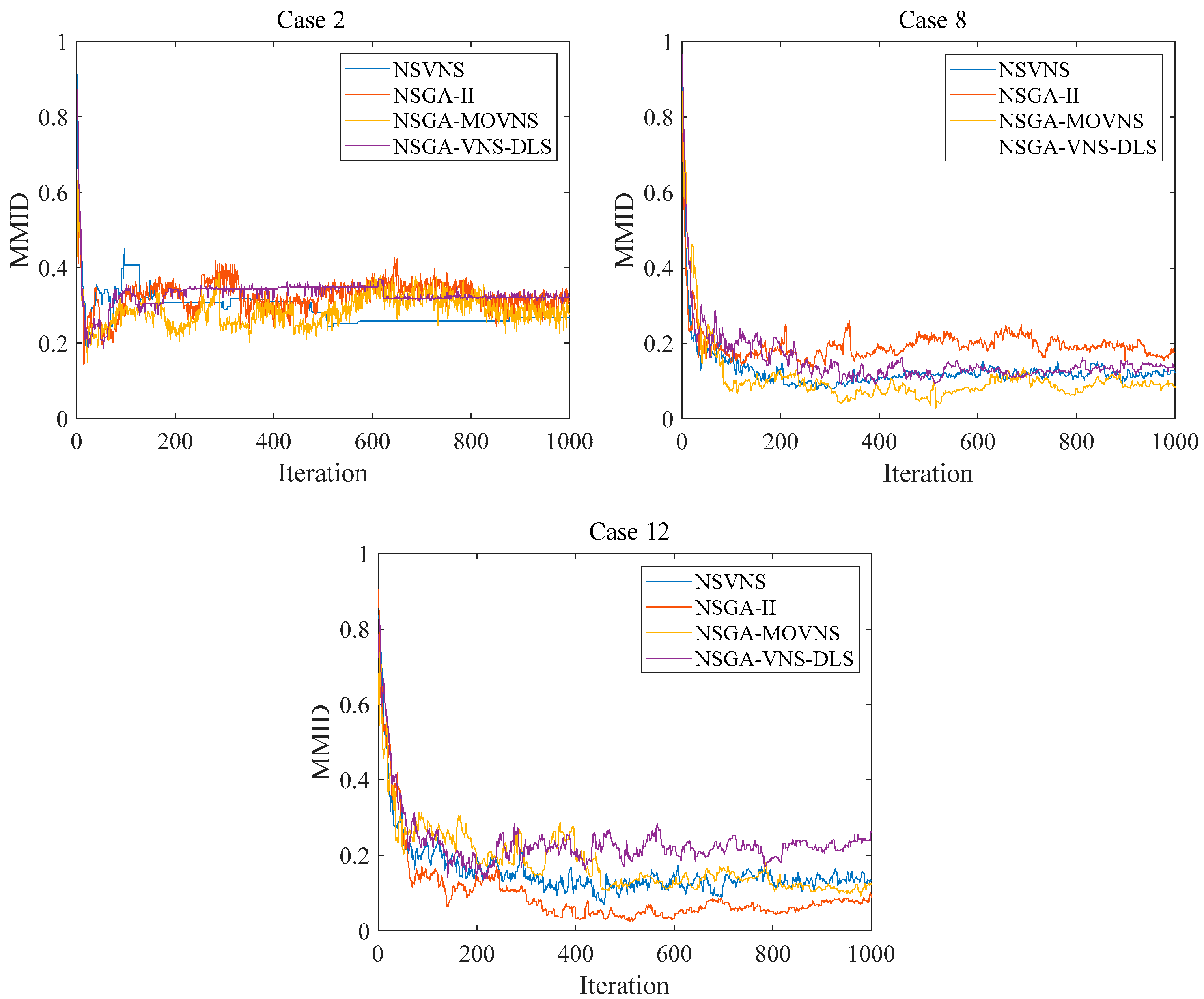
Larger NPS exhibits higher power of MOEAs to find more non-dominated solutions, and smaller MMID indicates more convergence strength of MOEAs. From both NPS and MMID perspectives, no significant difference exists between MOEAs as in Table 11. Figure 12. also verifies the similar convergence power of MOEAs by illustrating the average MMID measured within 1000 iterations over 10 runs for three case studies in different sizes. While Figure 11 shows different distributions of NPS and MMID in solving 12 case studies, the means of NPS and MMID are also similar and estimated at 5 and 0.3, respectively, for all MOEAs. However, NSGA-VNS-DLS slightly has a better performance in finding more non-dominated solutions (NPS) with a better convergence profile (MMID) for most case studies when compared with the other MOEAs as in Table 6 and Table 7. The external set defined in the NSVNS stage of NSGA-VNS-DLS may help this algorithm find more NPS. Also, the switch mechanism of NSGA-VNS-DLS from NSGA-II to NSVNS may contribute to more powerful convergence with less MMID. NSGA-VNS-DLS also significantly outperforms other MOEAs in terms of DM as in Table 11. The distribution of DM for NSGA-VNS-DLS also illustrates and confirms the results in Figure 11. In more detail, the efficacy of MOEAs is similar from Case 1 to 5. From Case 6 to 12, NSVNS-VNS-DLS is the best MOEA while NSVNS is the worst one in most cases as shown in Table 8. NSVNS shows relatively poor performance in most cases since it works with the MOVNS operator which empowers the neighborhood search (exploitation) instead of searching in the entire solution domain (exploration) to contribute to diverse Pareto-optimal frontiers with a better DM. On the contrary, NSGA-VNS-DLS addresses both exploration and exploitation using its switch mechanism between NSGA-II and NSVNS. This feature makes NSVNS-DLS-VNS the strongest algorithm to find diverse non-dominated solutions in most case studies.

On the one hand, the MOVNS operator introduced in Section 3.2 allows an MOEA to find new solutions within a specific distance in the search domain. Six predetermined neighborhood structures are defined for the MOVNS operator when discovering a new solution. Therefore, NSVNS, which is mainly designed based on the MOVNS, is the best algorithm in terms of SM to find non-dominated solutions with a consistent distance between them as seen in Table 11. Since NSGA-MOVNS and NSGA-VNS-DLS also employ the MOVNS operator with less concentration than NSVNS, they are placed in second and third ranks for SM as in Table 11. Last, NSGA-II is the worst algorithm in terms of SM due to a lack of the MOVNS operator as in Table 11. Table 9 and Figure 11 also explain the similar SM results for most case studies.

On the other hand, MOVNS is a significantly time-consuming operator since it needs to check and compare six neighborhood structures to find the best solutions. Thus, NSVNS, which uses MOVNS to create an external set at each iteration, significantly needs more time than other MOEAs as in Table 10 and Table 11. Following NSVNS, both NSGA-MOVNS and NSGA-VNS-DLS solve case studies in a shorter time since MOVNS does not play a key role in their structures as in Table 10 and Table 11. Furthermore, NSGA-II is the fastest MOEA as it does not have the MOVNS operator as shown in Table 10 and Table 11. In addition, Table 10 presents the computational complexity of the MOEAs since more complex algorithms would require a longer time to compute. Also, the distribution of CPU time in Figure 11 suggests the significant difference between NSGA-II and NSVNS.

To select the most efficient algorithm from the MOEAs in this study, we apply simple additive weighting (SAW) on RBD results by considering the same weight for all metrics. For this method, the values of one, two, and three are assigned to Tukey’s groups “B”, “A, B”, and “A”, respectively. The SAW scores are reported in Table 11 and show that NSGA-VNS-DLS with a SAW score of about 4.333 has the best overall performance.

4.4. Managerial Insights

In this subsection, we analyze the effects of four important problem parameters on total EC ($f_{EC}$) and OT ($f_{OT}$): the number of orders ($x_1$), number of SKUs for each order/order size ($x_2$), number of forklifts ($x_3$), and the number of battery chargings ($x_4$). A total of 71 Pareto-optimal frontiers are obtained by NSGA-VNS-DLS over 10 runs of all case studies, and we use these 71 frontiers for this analysis.

From the 71 Pareto-optimal frontiers, we also build 2 multiple linear regression (MLR) models for $f_{EC}$ and $f_{OT}$ as dependent variables to examine the effects of $x_1$, $x_2$, $x_3$, and $x_4$ on EC and OT. We apply a log transformation to the independent parameters ($x_1$, $x_2$, $x_3$, and $x_4$) to make the model residuals normally distributed. The initial MLR results have a multicollinearity issue as the order size ($x_2$) and the number of forklifts ($x_3$) are highly correlated with the variation inflation factor (VIF) $>10$. Thus, we make the final MLR models without $x_2$ for both $f_{EC}$ and $f_{OT}$.

Table 12. MLRs for EC (kWh).

$\mathbf{Regression} \mathbf{Equation}: {\mathit{f}}_{\mathit{E}\mathit{C}}={\mathit{b}}_0+{\mathit{b}}_1·\mathbf{ln}{\mathit{x}}_1+{\mathit{b}}_2·\mathbf{ln}{\mathit{x}}_2+{\mathit{b}}_3·\mathbf{ln}{\mathit{x}}_3+{\mathit{b}}_4·\mathbf{ln}{\mathit{x}}_4$
	Final Model
Terms	Coefficient	p-Value	VIF
Constant	−6.97391	0.0011	0
$\ln x_1$	4.02317	<0.0001	2.78592
$\ln x_2$	-	-	-
$\ln x_3$	3.31685	0.0066	1.78024
$\ln x_4$	0.45979	<0.0001	2.15809
$R^2$	0.8742

shows that $R^2$ is about 87%, and the result validates the reliability of the MLR for EC. In addition, all $x_1$, $x_3$, and $x_4$ are significant at a significance level of 0.05 ($p-value<0.05$).

Table 13. MLRs for OT (hour).

$\mathbf{Regression} \mathbf{Equation}: {\mathit{f}}_{\mathit{O}\mathit{T}}={\mathit{b}}_0+{\mathit{b}}_1·\mathbf{ln}{\mathit{x}}_1+{\mathit{b}}_2·\mathbf{ln}{\mathit{x}}_2+{\mathit{b}}_3·\mathbf{ln}{\mathit{x}}_3+{\mathit{b}}_4·\mathbf{ln}{\mathit{x}}_4$
	Final Model
Terms	Coefficient	p-Value	VIF
Constant	3.27696	0.8486	0
$\ln x_1$	18.50963	<0.0001	1.57369
$\ln x_2$	-	-	-
$\ln x_3$	-	-	-
$\ln x_4$	3.92938	<0.0001	1.57369
$R^2$	0.7741

presents that $x_1$ and $x_4$ are statistically significant ($p-value<0.05)$ while $x_3$ (number of forklifts) does not significantly affect $f_{OT}$. To construct a more accurate model for $f_{OT}$, we remove $x_3$ and obtain the final MLR, as shown in Table 13. $R^2$ of MLR of $f_{OT}$ is high ($77.41\%$), indicating that this MLR is also reliable.

In this regression analysis, we develop Equation (27) to evaluate the effects of independent parameters ($x_1$, $x_3$, and $x_4$) on EC ($f_{EC}$) and OT ($f_{OT}$) [48].

$${\rho }_i=b_i·\ln 1.01$$

(27)

$b_i$ is the coefficient of transformed $x_i$ from an MLR.

The absolute value of ${\rho }_i$ reflects the relative power of parameters $x_i$ to change $f_{EC}$ or $f_{OT}$. In other words, the absolute value of ${\rho }_i$ shows how much $f_{EC}$ or $f_{OT}$ changes by a one-percent change in the parameter $x_i$. In addition, the sign of ${\rho }_i$, which is the same as the sign of $b_i$, indicates a positive/negative correlation between the parameter $x_i$ and $f_{EC}$ or $f_{OT}$. From both EC and OT perspectives, the number of orders ($x_1$) is the most powerful parameter with a positive correlation when compared with the number of forklifts ($x_3$) and the number of battery charging ($x_4$), as shown in

Table 14. Effects of problem parameters on EC and OT.

1% Increase in Parameters	$\mathbf{Change} \mathbf{of} {\mathit{f}}_{\mathit{E}\mathit{C}}$ (kWH)	$\mathbf{Change} \mathbf{of} {\mathit{f}}_{\mathit{O}\mathit{T}}$ (h)
$1.01·x_1$	$b_1·\ln 1.01\approx$ 0.04003	$b_1·\ln 1.01\approx$ 0.18418
$1.01·x_3$	$b_3·\ln 1.01\approx$ 0.033	-
$1.01·x_4$	$b_4·\ln 1.01\approx$ 0.00457	$b_4·\ln 1.01\approx$ 0.0391

. Since more orders ($x_1$) requires more work from forklifts, the demand to recharge batteries increases by leading to more $f_{EC}$. In this case, forklifts also become less available when dealing with more orders in a tight time window, resulting in more $f_{OT}$. The second powerful parameter is the number of forklifts ($x_3$) in terms of EC. More forklifts ($x_3$) increases the number of charging ($x_4$), which eventually contributes to higher EC. Therefore, there is a positive correlation between $x_3$ and $f_{EC}$ or between $x_4$ and $f_{EC}$. Furthermore, more battery chargings ($x_4$) are needed as the least powerful parameter leads to a longer total charging time and less forklift availability, which increases both EC and OT.

One more thing to point out in Table 14 is that for the same 1% increase in both $x_1$ and $x_4$, the increase ratio of OT and EC (OT/EC) is much larger for $x_4$ (8.6 $\approx$0.0391/0.00457) than in $x_1$ (4.6 $\approx$ 0.18418/0.04003). In other words, for the same 1% increase in the number of orders ($x_1$) and number of battery chargings ($x_4$), OT proportionally increases more with the increase in $x_4$ than that in $x_1$. This suggests that warehouse decision makers should expect more increase in OT when the number of battery chargings ($x_4$) increases than when the number of orders ($x_1$) increases.

5. Conclusions

In this paper, EC and OT are studied as two minimization objective functions of a mixed-integer linear model proposed for a picker-to-parts system with fast charging technology. To fill a lack of study in the literature, the proposed model determines the battery charging scheduling of electric forklifts in conjunction with order batching, batch assignment, batch sequencing, and forklift routing problems. To make EC and OT analysis more realistic, we also measure the travel time of forklifts based on the A/D and velocity of the forklifts in different horizontal and vertical movement scenarios. In addition, empirical power data from horizontal and vertical movements of a forklift provided by a forklift manufacturer is used with the measured forklift travel time to estimate EC for case studies.

We use an AUGMECON method to verify the model by solving small-sized case studies. In addition, to deal with medium- to large-sized case studies, four MOEAs are presented. The performances of MOEAs are compared with each other and AUGMECON method, and the results exhibit that NSGA-VNS-DLS is selected as the most efficient algorithm. NSGA-VNS-DLS shows the best performance for all performance metrics: 5.299 (NPS), 0.288 (MMID), 13.013 (DM), 1.663 (SM), 2945.43, (CPU time), and 4.333 (overall avg). This suggests that the results from MOEAs performance analysis in this study can be applied to a variety of picker-to-parts warehouse optimization problems considering many variables, including the five important decisions from the literature: order batching, batch assignment, batch sequencing, forklift routing, and forklift battery charging. From the results of MLRs, the number of orders as the most significant parameter affects EC and OT with positive correlations of 4.0 (EC) and 18.5 (OT). The number of forklifts also significantly increases EC as the second significant parameter. Furthermore, the number of battery charging demonstrates a significant influence on both EC and OT with positive correlations. In addition, the same percentage increase in the number of orders and the number of battery charging results in more increase in OT than in EC with the number of battery charging increased, compared with the case of an increase in the number of orders. This study can help industrial practitioners and academic researchers find and analyze a relationship between EC and OT; for each warehouse configuration, warehouse operators can consider how much EC and OT increase or decrease together or individually for different warehouse settings, leading to more sustainable decisions in warehouses. While this study has also modeled the most important picker-to-parts problems and presented new MOEAs, other problems such as the storage location assignment or other algorithms in [49,50,51] deserve future research.

References

1. Petersen, C.G.; Schmenner, R.W. An Evaluation of Routing and Volume-Based Storage Policies in an Order Picking Operation. Decis. Sci. 1999, 30, 481–501. [Google Scholar] [CrossRef]
2. Ebrahimi, A.; Kia, R.; Komijan, A.R. Solving a Mathematical Model Integrating Unequal-Area Facilities Layout and Part Scheduling in a Cellular Manufacturing System by a Genetic Algorithm. SpringerPlus 2016, 5, 1254. [Google Scholar] [CrossRef] [PubMed] [Green Version]
3. Ebrahimi, A.; Jeon, H.W.; Lee, S.; Wang, C. Minimizing Total Energy Cost and Tardiness Penalty for a Scheduling-Layout Problem in a Flexible Job Shop System: A Comparison of Four Metaheuristic Algorithms. Comput. Ind. Eng. 2020, 141, 106295. [Google Scholar] [CrossRef]
4. Wäscher, G. Order Picking: A Survey of Planning Problems and Methods. In Supply Chain Management and Reverse Logistics; Dyckhoff, H., Lackes, R., Reese, J., Eds.; Springer: Berlin/Heidelberg, Germany, 2004; pp. 323–347. ISBN 978-3-540-24815-6. [Google Scholar]
5. Kutkut, N. Is Fast Charging for You? Mater. Handl. Manag. 2005, 62. Available online: https://www.mhlnews.com/powered-vehicles-and-forklifts/article/22040185/is-fast-charging-for-you (accessed on 10 March 2023).
6. Carli, R.; Dotoli, M.; Digiesi, S.; Facchini, F.; Mossa, G. Sustainable Scheduling of Material Handling Activities in Labor-Intensive Warehouses: A Decision and Control Model. Sustainability 2020, 12, 3111. [Google Scholar] [CrossRef] [Green Version]
7. Henn, S.; Wäscher, G. Tabu Search Heuristics for the Order Batching Problem in Manual Order Picking Systems. Eur. J. Oper. Res. 2012, 222, 484–494. [Google Scholar] [CrossRef] [Green Version]
8. Henn, S.; Schmid, V. Metaheuristics for Order Batching and Sequencing in Manual Order Picking Systems. Comput. Ind. Eng. 2013, 66, 338–351. [Google Scholar] [CrossRef]
9. Chen, T.-L.; Cheng, C.-Y.; Chen, Y.-Y.; Chan, L.-K. An Efficient Hybrid Algorithm for Integrated Order Batching, Sequencing and Routing Problem. Int. J. Prod. Econ. 2015, 159, 158–167. [Google Scholar] [CrossRef]
10. Cheng, C.-Y.; Chen, Y.-Y.; Chen, T.-L.; Yoo, J.J.-W. Using a Hybrid Approach Based on the Particle Swarm Optimization and Ant Colony Optimization to Solve a Joint Order Batching and Picker Routing Problem. Int. J. Prod. Econ. 2015, 170, 805–814. [Google Scholar] [CrossRef]
11. Henn, S. Order Batching and Sequencing for the Minimization of the Total Tardiness in Picker-to-Part Warehouses. Flex. Serv. Manuf. J. 2015, 27, 86–114. [Google Scholar] [CrossRef]
12. Muter, İ.; Öncan, T. An Exact Solution Approach for the Order Batching Problem. IIE Trans. 2015, 47, 728–738. [Google Scholar] [CrossRef]
13. Fekete, P.; Lim, S.; Martin, S.; Kuhn, K.; Wright, N. Improved Energy Supply for Non-Road Electric Vehicles by Occasional Charging Station Location Modelling. Energy 2016, 114, 1033–1040. [Google Scholar] [CrossRef]
14. Ardjmand, E.; Huh, D.W. Coordinated Warehouse Order Picking and Production Scheduling: A NSGA-II Approach. In Proceedings of the 2017 IEEE Symposium Series on Computational Intelligence (SSCI), Honolulu, HI, USA, 27 November–1 December 2017; pp. 1–8. [Google Scholar]
15. Li, J.; Huang, R.; Dai, J.B. Joint Optimisation of Order Batching and Picker Routing in the Online Retailer’s Warehouse in China. Int. J. Prod. Res. 2017, 55, 447–461. [Google Scholar] [CrossRef]
16. Scholz, A.; Schubert, D.; Wäscher, G. Order Picking with Multiple Pickers and Due Dates–Simultaneous Solution of Order Batching, Batch Assignment and Sequencing, and Picker Routing Problems. Eur. J. Oper. Res. 2017, 263, 461–478. [Google Scholar] [CrossRef] [Green Version]
17. Menéndez, B.; Bustillo, M.; Pardo, E.G.; Duarte, A. General Variable Neighborhood Search for the Order Batching and Sequencing Problem. Eur. J. Oper. Res. 2017, 263, 82–93. [Google Scholar] [CrossRef]
18. Ardjmand, E.; Shakeri, H.; Singh, M.; Bajgiran, O.S. Minimizing Order Picking Makespan with Multiple Pickers in a Wave Picking Warehouse. Int. J. Prod. Econ. 2018, 206, 169–183. [Google Scholar] [CrossRef]
19. Žulj, I.; Kramer, S.; Schneider, M. A Hybrid of Adaptive Large Neighborhood Search and Tabu Search for the Order-Batching Problem. Eur. J. Oper. Res. 2018, 264, 653–664. [Google Scholar] [CrossRef]
20. Pinto, A.R.F.; Nagano, M.S. An Approach for the Solution to Order Batching and Sequencing in Picking Systems. Prod. Eng. 2019, 13, 325–341. [Google Scholar] [CrossRef]
21. Kuhn, H.; Schubert, D.; Holzapfel, A. Integrated Order Batching and Vehicle Routing Operations in Grocery Retail—A General Adaptive Large Neighborhood Search Algorithm. Eur. J. Oper. Res. 2020, 294, 1003–1021. [Google Scholar] [CrossRef]
22. Lee, I.G.; Chung, S.H.; Yoon, S.W. Two-Stage Storage Assignment to Minimize Travel Time and Congestion for Warehouse Order Picking Operations. Comput. Ind. Eng. 2020, 139, 106129. [Google Scholar] [CrossRef]
23. Yang, P.; Zhao, Z.; Guo, H. Order Batch Picking Optimization under Different Storage Scenarios for E-Commerce Warehouses. Transp. Res. Part E Logist. Transp. Rev. 2020, 136, 101897. [Google Scholar] [CrossRef]
24. Cano, J.A.; Cortés, P.; Campo, E.A.; Correa-Espinal, A.A. Multi-objective grouping genetic algorithm for the joint order batching, batch assignment, and sequencing problem. Int. J. Manag. Sci. Eng. Manag. 2021, 17, 188–204. [Google Scholar] [CrossRef]
25. Dauod, H.; Won, D. Real-Time Order Picking Planning Framework for Warehouses and Distribution Centres. Int. J. Prod. Res. 2021, 60, 5468–5487. [Google Scholar] [CrossRef]
26. Karimi-Mamaghan, M.; Mohammadi, M.; Pasdeloup, B.; Meyer, P. Learning to Select Operators in Meta-Heuristics: An Integration of Q-Learning into the Iterated Greedy Algorithm for the Permutation Flowshop Scheduling Problem. Eur. J. Oper. Res. 2023, 304, 1296–1330. [Google Scholar] [CrossRef]
27. Mavrotas, G. Effective Implementation of the ε-Constraint Method in Multi-Objective Mathematical Programming Problems. Appl. Math. Comput. 2009, 213, 455–465. [Google Scholar] [CrossRef]
28. Zhang, J.; Zhang, N.; Tian, L.; Zhou, Z.; Wang, P. Robots’ Picking Efficiency and Pickers’ Energy Expenditure: The Item Storage Assignment Policy in Robotic Mobile Fulfillment System. Comput. Ind. Eng. 2023, 176, 108918. [Google Scholar] [CrossRef]
29. Yusoff, Y.; Ngadiman, M.S.; Zain, A.M. Overview of NSGA-II for Optimizing Machining Process Parameters. Procedia Eng. 2011, 15, 3978–3983. [Google Scholar] [CrossRef] [Green Version]
30. Lv, L.; Shen, W. An Improved NSGA-II with Local Search for Multi-Objective Integrated Production and Inventory Scheduling Problem. J. Manuf. Syst. 2023, 68, 99–116. [Google Scholar] [CrossRef]
31. Lesch, V.; Müller, P.B.; Krämer, M.; Hadry, M.; Kounev, S.; Krupitzer, C. Optimizing Storage Assignment, Order Picking, and Their Interaction in Mezzanine Warehouses. Appl. Intell. 2023, 1–25. [Google Scholar] [CrossRef]
32. Wang, Q.; Li, H.; Wang, D.; Cheng, T.C.E.; Yin, Y. Bi-Objective Perishable Product Delivery Routing Problem with Stochastic Demand. Comput. Ind. Eng. 2023, 175, 108837. [Google Scholar] [CrossRef]
33. Min, C.; Pan, Y.; Dai, W.; Kawsar, I.; Li, Z.; Wang, G. Trajectory Optimization of an Electric Vehicle with Minimum Energy Consumption Using Inverse Dynamics Model and Servo Constraints. Mech. Mach. Theory 2023, 181, 105185. [Google Scholar] [CrossRef]
34. Yao, Z.; Yoon, H.-S.; Hong, Y.-K. Control of Hybrid Electric Vehicle Powertrain Using Offline-Online Hybrid Reinforcement Learning. Energies 2023, 16, 652. [Google Scholar] [CrossRef]
35. Cao, B.; Yan, Y.; Wang, Y.; Liu, X.; Lin, J.C.-W.; Sangaiah, A.K.; Lv, Z. A Multiobjective Intelligent Decision-Making Method for Multistage Placement of PMU in Power Grid Enterprises. IEEE Trans. Ind. Inform. 2023, 19, 7636–7644. [Google Scholar] [CrossRef]
36. TMHNA. Available online: https://www.tmhna.com/ (accessed on 19 March 2023).
37. Deb, K.; Pratap, A.; Agarwal, S.; Meyarivan, T. A Fast and Elitist Multiobjective Genetic Algorithm: NSGA-II. IEEE Trans. Evol. Comput. 2002, 6, 182–197. [Google Scholar] [CrossRef] [Green Version]
38. Mladenović, N.; Hansen, P. Variable Neighborhood Search. Comput. Oper. Res. 1997, 24, 1097–1100. [Google Scholar] [CrossRef]
39. Taguchi, G. Introduction to Quality Engineering: Designing Quality into Products and Processes; Asian Productivity Organization: Tokyo, Japan, 1986. [Google Scholar]
40. Maghsoudlou, H.; Kahag, M.R.; Niaki, S.T.A.; Pourvaziri, H. Bi-Objective Optimization of a Three-Echelon Multi-Server Supply-Chain Problem in Congested Systems: Modeling and Solution. Comput. Ind. Eng. 2016, 99, 41–62. [Google Scholar] [CrossRef]
41. Rahmati, S.H.A.; Hajipour, V.; Niaki, S.T.A. A Soft-Computing Pareto-Based Meta-Heuristic Algorithm for a Multi-Objective Multi-Server Facility Location Problem. Appl. Soft Comput. 2013, 13, 1728–1740. [Google Scholar] [CrossRef]
42. Karimi, N.; Zandieh, M.; Karamooz, H.R. Bi-Objective Group Scheduling in Hybrid Flexible Flowshop: A Multi-Phase Approach. Expert Syst. Appl. 2010, 37, 4024–4032. [Google Scholar] [CrossRef]
43. Zitzler, E. Evolutionary Algorithms for Multiobjective Optimization: Methods and Applications. Ph.D. Thesis, Swiss Federal Institute of Technology Zurich, Zurich, Switzerland, 1999. [Google Scholar]
44. Elsayed, E.A.; Lee, M.-K. Order Processing in Automated Storage/Retrieval Systems with Due Dates. IIE Trans. 1996, 28, 567–577. [Google Scholar] [CrossRef]
45. Parks, B. Forklift Batteries: Conventional vs. Fast vs. Opportunity Charging. Available online: https://www.tmhnc.com/blog/forklift-battery-charging-fast-opportunity-conventional (accessed on 24 November 2020).
46. Hwang, H.; Lee, S.B. Travel-Time Models Considering the Operating Characteristics of the Storage and Retrieval Machine. Int. J. Prod. Res. 1990, 28, 1779–1789. [Google Scholar] [CrossRef]
47. Schott, J.R. Fault Tolerant Design Using Single and Multicriteria Genetic Algorithm Optimization. Ph.D. Thesis, Massachusetts Institute of Technology, Cambridge, MA, USA, 1995. [Google Scholar]
48. Benoit, K. Linear Regression Models with Logarithmic Transformations; London School of Economics: London, UK, 2011; Volume 22, pp. 23–36. [Google Scholar]
49. Zhao, H.; Zhang, C. An Online-Learning-Based Evolutionary Many-Objective Algorithm. Inf. Sci. 2020, 509, 1–21. [Google Scholar] [CrossRef]
50. Dulebenets, M.A. An Adaptive Polyploid Memetic Algorithm for Scheduling Trucks at a Cross-Docking Terminal. Inf. Sci. 2021, 565, 390–421. [Google Scholar] [CrossRef]
51. Dulebenets, M.A.; Kavoosi, M.; Abioye, O.; Pasha, J. A Self-Adaptive Evolutionary Algorithm for the Berth Scheduling Problem: Towards Efficient Parameter Control. Algorithms 2018, 11, 100. [Google Scholar] [CrossRef] [Green Version]
Figure 1. Relationships and effects of important parameters and variables on EC and OT.
Sustainability 15 10551 g001
Figure 2. Illustrative example of solution representation and six neighborhood structures.
Sustainability 15 10551 g002
Figure 3. Mechanism of NSVNS.
Sustainability 15 10551 g003
Figure 4. Mechanism of NSGA-MOVNS.
Sustainability 15 10551 g004
Figure 5. Pareto fronts of MOEAs obtained for medium-sized case study over 10 runs.
Sustainability 15 10551 g005
Figure 6. Main effects plots for S/N ratios of MOEAs.
Sustainability 15 10551 g006
Figure 7. Bird’s eye view of picker-to-parts system layout.
Sustainability 15 10551 g007
Figure 8. Forklift travel scenarios.
Sustainability 15 10551 g008
Figure 9. Combination of travel scenarios.
Sustainability 15 10551 g009
Figure 10. EC illustration in horizontal and vertical movements.
Sustainability 15 10551 g010
Figure 11. Box and whisker plots for four MOEAs.
Sustainability 15 10551 g011
Figure 12. Convergence profiles of MOEAs for MMID (smaller is better).
Sustainability 15 10551 g012