A Novel Odd Beta Prime-Logistic Distribution: Desirable Mathematical Properties and Applications to Engineering and Environmental Data

Abstract

In parametric statistical modeling, it is important to construct new extensions of existing probability distributions (PDs) that can make modeling data more flexible and help stakeholders make better decisions. In the present study, a new family of probability distributions (FPDs) called the odd beta prime generalized (OBP-G) FPDs is proposed to improve the traditional PDs. A new PD called the odd beta prime-logistic (OBP-logistic) distribution has been developed based on the developed OBP-G FPDs. Some desirable mathematical properties of the proposed OBP-logistic distribution, including the moments, moment-generating function, information-generating function, quantile function, stress–strength, order statistics, and entropies, are studied and derived. The proposed OBP-logistic distribution’s parameters are determined by adopting the maximum likelihood estimation (MLE) method. The applicability of the new PD was demonstrated by employing three data sets and these were compared by the known extended logistic distributions, such as the gamma generalized logistic distribution, new modified exponential logistic distribution, gamma-logistic distribution, exponential modified Weibull logistic distribution, exponentiated Weibull logistic distribution, and transmuted Weibull logistic distribution. The findings reveal that the studied distribution provides better results than the competing PDs. The empirical results showed that the new OBP-logistic distribution performs better than the other PDs based on several statistical metrics. We hoped that the newly constructed OBP-logistic distribution would be an alternative to other well-known extended logistic distributions for the statistical modeling of symmetric and skewed data sets.

1. Introduction

The probability distributions (PDs) are vital statistical tools for modeling the underlying behavior of a given data set collected from surveys, observational studies, experiments, and more. In many practical scenarios, most of these PDs are not suitable to fit every characteristic of real phenomenon. However, statistical literature lacks a standard PD model that can adequately suit every kind of phenomenon [1,2,3]. Therefore, it is imperative to establish new PDs that can provide better flexibility, which can be achieved by adding one or more parameters to the well-established PDs [4]. In recent times, there has been a gradual emergence of new FPDs developed for data modelling in many practical domains, such as the environment, finance, engineering, and biological sciences. Some of the well-known methods for generating new PDs are included in [5,6,7,8,9,10,11,12,13,14,15,16,17,18,19,20]. Other methods to generate flexible PDs are the odd generalized NH-G [21], Marshall–Olkin odd Lindley-G [22], Maxwell-G [23], odd inverse power generalized Weibull-G [24], generalized Rayleigh-G [25], generalized odd linear exponential-G [26], generalized exponential extended exponentiated-G [27] and generalized alpha exponent power-G [28], among others.

In this paper, we introduced a novel FPD derived using the beta prime (BP) distribution, popularly known as the beta of the second kind, Feller–Pareto, the Pearson Type VI, or generalized F distribution [29,30,31]. However, few studies have looked into the application of BP distribution [29]. For instance, the distribution of taxed income in Finland was fitted by [32] using a four-parameter BP distribution. The findings indicated that their proposed distribution performed better than the two- and three-parameter log-normal distributions. The study by [33] estimated the BP distribution for family incomes in the United States, while [34] determined the parameters via the maximum likelihood estimation (MLE) method and studied its properties. Moreover, the application of BP distribution was utilized by [35,36] to study regression models for positive random variables (RVs). As defined in [29,37,38], the BP has the following cumulative distribution function (cdf):

$$\mathrm{W}\left(\mathrm{x};\mathrm{a},\mathrm{b}\right)={\mathrm{I}}_{\frac{\mathrm{x}}{\left(1+\mathrm{x}\right)}}\mathrm{B}\left(\mathrm{a},\mathrm{b}\right), \mathrm{x}>0, \mathrm{a},\mathrm{b}>0,$$

(1)

where ${\mathrm{B}}_{\mathrm{x}}\left(\mathrm{a},\mathrm{b}\right)={\displaystyle \underset{0}{\overset{\mathrm{x}}{\int }}{\mathsf{\omega }}^{\mathrm{a}-1}{\left(1-\mathsf{\omega }\right)}^{\mathrm{b}-1}\mathrm{d}\mathsf{\omega }}$ is the incomplete beta function.

The associated probability density function (pdf) is defined as

$$\mathrm{w}(\mathrm{x};\mathrm{a},\mathrm{b})=\frac{1}{\mathrm{B}\left(\mathrm{a},\mathrm{b}\right)}\frac{{\mathrm{x}}^{\mathrm{a}-1}}{{\left(1+\mathrm{x}\right)}^{\mathrm{a}+\mathrm{b}}}, \mathrm{x}>0.$$

(2)

The logistic distribution (LD) is a univariate continuous PD for modeling data in diverse contexts, including life sciences, physical sciences, sports, finance, insurance, neural networks, logit models, logistic regression, and recently, machine learning. This distribution is more flexible to the underlying data involving extreme events and has a fatter tail than a normal distribution suitable for modeling returns in the stock market [39]. Due to its convenience and significance, the LD is regarded by numerous researchers as a growth curve. For example, studies by [40,41] used LD in human populations and some biological organisms. Another study by [42] applied LD to data associated with the agricultural population. Another important application of the LD is in the analysis of survival data [43]. More interesting practical applications of the LD can be found in [44] and the references therein. The cdf of the LD is expressed as

$$\mathrm{P}(\mathrm{x};\mathsf{\mu },\mathrm{s})=\frac{1}{1+\exp -\left(\frac{\mathrm{x}-\mathsf{\mu }}{\mathrm{s}}\right)}, \mathrm{x},\mathsf{\mu }\in ℝ, \mathrm{s}>0.$$

(3)

The pdf of the LD corresponding to (3) is defined as

$$\mathrm{P}(\mathrm{x};\mathsf{\mu },\mathrm{s})=\frac{\exp -\left(\frac{\mathrm{x}-\mathsf{\mu }}{\mathrm{s}}\right)}{\mathrm{s}{\left(1+\exp -\left(\frac{\mathrm{x}-\mathsf{\mu }}{\mathrm{s}}\right)\right)}^2}, \mathrm{x},\mathsf{\mu }\in ℝ, \mathrm{s}>0,$$

(4)

where $\mathsf{\mu }$ is the location parameter and $\mathrm{s}$ is the scale parameter.

Several generalizations of the LD have been introduced in the literature to study its properties and examine its adaptability and flexibility in modeling skewed data [45]. These generalizations are essential to enhance the fit in the non-central probability regions and to improve the use of LD regarding the asymmetric probability curves [46]. For example, Ref. [47] introduced the LD of type IV and applied it to study binomial regression data. In [48], the logistic regression model was proposed. Ref. [49] proposed three generalizations of LD types. Comprehensive generalizations of the LD have been studied and summarized [44]. The skewed LD was proposed [50]. An extended version of the LD was developed and studied [51] by adding a new parameter. Two extended versions of skewed LD have been established [52] using the method proposed and defined by [53]. The two widely used approaches to derive different generalizations of PDs, including the LD [54], are the T-X framework studied by [55] and modified by [56]. The exponentiated exponential LD was recently established by [57], and several of its properties where defined and derived.

Recently, Ref. [9] introduced a technique for generalizing FPDs with the cdf defined by

$$\mathrm{F}(\mathrm{x})={\displaystyle \underset{\mathrm{a}}{\overset{\mathrm{W}\left(\mathrm{Q}(\mathrm{x})\right)}{\int }}\mathrm{v}(\mathrm{m})\mathrm{d}\mathrm{m}}=\mathrm{M}\left\{\mathrm{W}\left(\mathrm{Q}(\mathrm{x})\right)\right\},$$

(5)

where $\mathrm{M}$ is an RV, $\mathrm{v}$ is the pdf of the RV $\mathrm{M}\in \left[\mathrm{a},\mathrm{b}\right]$, such that $-\infty \le \mathrm{a}<\mathrm{b}\le \infty$ and $\mathrm{W}\left(\mathrm{Q}(\mathrm{x})\right)$ is a link function of any cdf of continuous PDs that takes different forms (see [55]). If we consider the odd function form, $\mathrm{W}\left(\mathrm{Q}(\mathrm{x})\right)=\frac{\mathrm{Q}(\mathrm{x})}{1-\mathrm{Q}(\mathrm{x})}$, then the cdf will be

$$\mathrm{F}(\mathrm{x})={\displaystyle \underset{0}{\overset{\frac{\mathrm{Q}(\mathrm{x})}{1-\mathrm{Q}(\mathrm{x})}}{\int }}\mathrm{v}(\mathrm{m})\mathrm{d}\mathrm{m}}=\mathrm{M}\left\{\frac{\mathrm{Q}(\mathrm{x})}{1-\mathrm{Q}(\mathrm{x})}\right\}.$$

(6)

Overall, the quest for high-tailed models is motivated by their capacity to offer more precise and realistic representations of extreme occurrences, enabling better risk management, financial modeling, hedging strategies, insurance evaluations, systemic risk analysis, and climate science. By developing models that can accurately represent extreme values, decision-makers can better understand and manage risks, make informed choices, and improve the overall robustness of their systems.

The justifications of this paper are as follows:

(i)

To define novel FPDs using the BP distribution.

(ii)

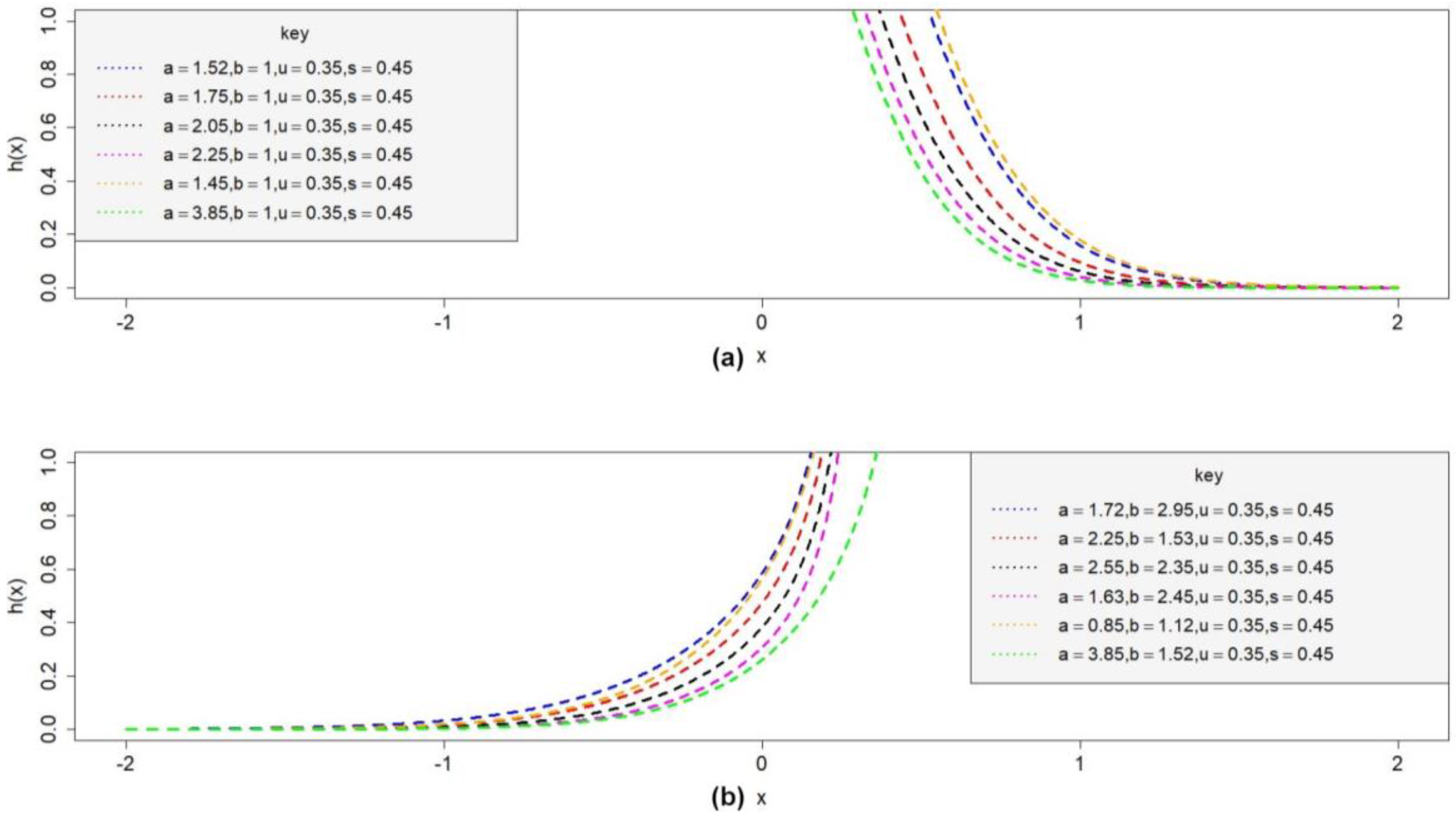
To develop new PD that can accommodate both monotonic and non-monotonic hazard rates.

(iii)

To establish heavy-tailed models for different data sets.

(iv)

To generate a PD that can provide suitable shapes to fit symmetric and skewed real data sets that are commonly found in practical disciplines, including environment, engineering, and finance.

(v)

To obtain a flexible PD that can consistently provide more realistic fits to given data sets when tested against known competing PDs.

The present paper is an extended version of our previously published conference paper [58]. However, this article expands upon the conference paper by providing more detailed derivations, analyses, and presenting a more comprehensive discussion and interpretation of the results. Moreover, the present article includes additional sections, such as an expanded introduction, literature review, validity test for the proposed family, new extension of LD and its properties, simulation studies and conclusion, which were not present in the conference paper.

The remaining parts of the paper are sectioned as follows: Section 2 highlights the related literature review. Section 3 introduces a novel odd beta prime FPD along with its cdf, pdf, validity test, and mixture representations. In Section 4, a special odd beta prime generalized LD is presented. Several statistical features of the new PD are studied and derived in Section 5. Section 6 describes the parameter estimation of the proposed PD by adopting the MLE approach. Section 7 contains Monte Carlo simulation to assess the estimators’ accuracy. Section 8 proves the usefulness of the constructed PD using three data sets. Discussion is presented in Section 9. Section 10 is reserved for conclusions.

2. Literature Review

Many efforts have been made to generate new FPD that expand the established classical PDs to increase the flexibility of modeling data in real-life applications. Several developed families have been adopted and applied to modeling diverse data types with varied characteristics. Many families of probability distributions were established using various approaches in the statistical literature. In this section, we have reviewed some recent families of distributions alongside their sub-models.

Bell generalized FPD was introduced by [59]. Bell Weibull (BellW), a unique model of this family, was first introduced. Some properties of this model were derived. The numerical demonstration was used to evaluate several actuarial measures for the BellW distribution. The significance of the proposed model was verified based on finance and medical data sets.

The unit exponentiated half logistic power series (UEHLPS) FPD was proposed by [60]. Several special models of this family were introduced, including the UEHL Poisson, UEHL Geometric, UEHL Binomial, and UEHL Logarithmic models. The general properties were derived. The parameter estimation for the UEHLP model was performed based on various classical estimation methods. A numerical simulation was utilized to examine the estimators’ accuracy. The usefulness of the UEHLP distribution was evaluated by analyzing the COVID-19, milk production, and failure data sets.

A new extended cosine generalized FPD was constructed by [61]. Some statistical features were obtained. Several sub-models of this family were introduced. The Bayesian and non-Bayesian approaches were adopted for parameter estimation. A simulation study was conducted to evaluate these approaches and demonstrate their practicality. The significance of the proposed models was assessed based on the three data sets, such as the lifetimes of devices, carbon fibers, and the single fibers.

The sine-exponentiated Weibull generalized FPD was pioneered by [62] based on the sine generalized and exponentiated Weibull generalized FPDs. Several properties of the developed distributions were obtained. Six different techniques of estimation were employed to estimate the parameters. The adequacy of these techniques was verified using Monte Carlo simulations. The significance of the family was analyzed based on five real data sets. The developed distribution was quite flexible compared to several well-established distributions.

The type II half-logistic odd Fréchet generalized FPD was constructed by [63] based on the classical Fréchet family. This family was used to produce symmetrical and asymmetrical special models. The new models are produced by this family. Some mathematical features of this family were derived. The estimate of the parameters was performed based on six distinct techniques. The Monte Carlo simulation study was employed to test these estimation techniques. The model was explored to analyze the real-word data sets involving biomedical, engineering, environment, and strength failure.

The odd Perks generalized FPD was studied by [64]. Four different special models of this family were examined, including the odd Perks uniform, odd Perks exponential, odd Perks Weibull, and odd Perks Lomax models. Some essential features of the proposed family were derived. The Bayesian and non-Bayesian methods were applied to estimate the model parameters. The odd Perks Weibull was explored to propose a new log-location-scale regression model. Several data sets were employed to verify the relevance and significance of the introduced distributions.

The truncated Cauchy power Weibull generalized FPD was generated by [65]. This family was used to establish three special models, such as the truncated Cauchy power Weibull Lomax, truncated Cauchy power Weibull exponential, and truncated Cauchy power Weibull Rayleigh models. Various properties of this family were discussed. The parameters were estimated based on the MLE and Bayesian techniques using censored data. The adequacy of the estimators was assessed using Monte Carlo simulation. The importance of the family was illustrated by fitting the three members of this family to three real datasets. The result revealed that the members of the family performed better compared to comparator models, suggesting that the members of the family provided a better fit.

The type I half logistic Burr X generalized FPD was introduced by [66]. Three sub-models of this family were introduced. Some important features of this family were obtained. The parameter estimators were produced using the MLE and Bayesian techniques using the type II censored data. The estimators were evaluated using Monte Carlo simulation. Three medical data sets from various countries were used to validate the goodness of the new models.

3. Development of Odd Beta Prime Generalized Family of Distributions

Here, we highlight the development of the novel generalized family of BP distributions using the method defined by [9] named the odd beta prime generalized (OBP-G) FPDs. The cdf of OBP-G FPDs will be developed by substituting the pdf in (6) with the pdf given in (2) as follows:

$$\begin{array}{ll}\mathrm{F}\left(\mathrm{x};\mathrm{a},\mathrm{b},\mathsf{\eta }\right)& =\frac{1}{\mathrm{B}\left(\mathrm{a},\mathrm{b}\right)}{\displaystyle \underset{0}{\overset{\frac{\mathrm{Q}\left(\mathrm{x};\mathsf{\eta }\right)}{1-\mathrm{Q}\left(\mathrm{x};\mathsf{\eta }\right)}}{\int }}\frac{{\mathrm{t}}^{\mathrm{a}-1}}{{\left(1+\mathrm{t}\right)}^{\mathrm{a}+\mathrm{b}}}}\mathrm{d}\mathrm{t},\\ & =\frac{ {\mathrm{B}}_{\frac{\mathrm{Q}\left(\mathrm{x};\mathsf{\eta }\right)}{1-\mathrm{Q}\left(\mathrm{x};\mathsf{\eta }\right)}}\left(\mathrm{a},\mathrm{b}\right)}{\mathrm{B}\left(\mathrm{a},\mathrm{b}\right)}; \mathrm{t}>0, \mathrm{a}>0,\mathrm{b}>0, \mathsf{\eta }\in ℝ,\end{array}$$

(7)

where $\mathrm{Q}\left(.;\mathsf{\eta }\right)$ is a cdf of a baseline distribution with the vector parameter $\mathsf{\eta }$. The associated pdf of OBP-G FPDs is obtained by differentiating (7) as

$$\begin{array}{ll}\mathrm{f}\left(\mathrm{x};\mathrm{a},\mathrm{b},\mathsf{\eta }\right)& =\frac{\mathrm{d}}{\mathrm{d}\mathrm{x}}\left[\mathrm{F}\left(\mathrm{x};\mathrm{a},\mathrm{b},\mathsf{\eta }\right)\right]=\frac{1}{\mathrm{B}\left(\mathrm{a},\mathrm{b}\right)} \frac{\mathrm{d}}{\mathrm{d}\mathrm{x}}\left({\mathrm{B}}_{\frac{\mathrm{Q}\left(\mathrm{x};\mathsf{\eta }\right)}{1-\mathrm{Q}\left(\mathrm{x};\mathsf{\eta }\right)}}\left(\mathrm{a},\mathrm{b}\right)\right),\\ & =\frac{1}{\mathrm{B}\left(\mathrm{a},\mathrm{b}\right)} \left[\frac{{\left(\frac{\mathrm{Q}\left(\mathrm{x};\mathsf{\eta }\right)}{1-\mathrm{Q}\left(\mathrm{x};\mathsf{\eta }\right)}\right)}^{\mathrm{a}-1}}{{\left[1+\left(\frac{\mathrm{Q}\left(\mathrm{x};\mathsf{\eta }\right)}{1-\mathrm{Q}\left(\mathrm{x};\mathsf{\eta }\right)}\right)\right]}^{\mathrm{a}+\mathrm{b}}} \frac{\mathrm{d}}{\mathrm{d}\mathrm{x}}\left(\frac{\mathrm{Q}\left(\mathrm{x};\mathsf{\eta }\right)}{1-\mathrm{Q}\left(\mathrm{x};\mathsf{\eta }\right)}\right)\right]; \mathrm{x}>0, \mathrm{a}>0, \mathrm{b}>0, \mathsf{\eta }\in ℝ.\end{array}$$

(8)

After simplifications, the pdf of (8) is

$$\mathrm{f}\left(\mathrm{x};\mathrm{a},\mathrm{b},\mathsf{\eta }\right)=\frac{\mathrm{q}\left(\mathrm{x};\mathsf{\eta }\right)}{\mathrm{B}\left(\mathrm{a},\mathrm{b}\right){\left(1-\mathrm{Q}\left(\mathrm{x};\mathsf{\eta }\right)\right)}^2}\frac{{\left(\frac{\mathrm{Q}\left(\mathrm{x};\mathsf{\eta }\right)}{1-\mathrm{Q}\left(\mathrm{x};\mathsf{\eta }\right)}\right)}^{\mathrm{a}-1}}{{\left[1+\left(\frac{\mathrm{Q}\left(\mathrm{x};\mathsf{\eta }\right)}{1-\mathrm{Q}\left(\mathrm{x};\mathsf{\eta }\right)}\right)\right]}^{\mathrm{a}+\mathrm{b}}}, \mathrm{x}>0, \mathrm{a}>0,\mathrm{b}>0, \mathsf{\eta }\in ℝ,$$

(9)

where $\mathrm{q}\left(.;\mathsf{\eta }\right)$ is the pdf of the baseline model $\mathrm{Q}\left(.;\mathsf{\eta }\right)$.

Henceforth, the RV $\mathrm{X}$ with the pdf given in (9) will be presented by $\mathrm{X}\sim \mathrm{O}\mathrm{B}\mathrm{P}-\mathrm{G}$. We omit the dependence on parameters $\mathrm{a},\mathrm{b}$ and $\mathsf{\eta }$ from (7) and (9) by denoting $\mathrm{F}\left(\mathrm{x};\mathrm{a},\mathrm{b},\mathsf{\eta }\right)=\mathrm{F}\left(\mathrm{x}\right)$ and $\mathrm{f}\left(\mathrm{x};\mathrm{a},\mathrm{b},\mathsf{\eta }\right)=\mathrm{f}\left(\mathrm{x}\right)$, respectively.

To verify whether the new OBP-G family is a valid FPD, the pdf given in (9) is used to satisfy the ${\displaystyle \underset{-\infty }{\overset{\infty }{\int }}\mathrm{f}(\mathrm{x})}\mathrm{d}\mathrm{x}=1$, where $\mathrm{f}$ is the pdf of OBP-G FPDs. For the sake of validation, we provide clear proof as follows:

$${\displaystyle \underset{-\infty }{\overset{\infty }{\int }}\mathrm{f}(\mathrm{x})\mathrm{d}\mathrm{x}}=\frac{1}{\mathrm{B}\left(\mathrm{a},\mathrm{b}\right)}{\displaystyle \underset{0}{\overset{\infty }{\int }}\frac{\mathrm{q}\left(\mathrm{x};\mathsf{\eta }\right)}{{\left(1-\mathrm{Q}\left(\mathrm{x};\mathsf{\eta }\right)\right)}^2}\frac{{\left(\frac{\mathrm{Q}\left(\mathrm{x};\mathsf{\eta }\right)}{1-\mathrm{Q}\left(\mathrm{x};\mathsf{\eta }\right)}\right)}^{\mathrm{a}-1}}{{\left[1+\left(\frac{\mathrm{Q}\left(\mathrm{x};\mathsf{\eta }\right)}{1-\mathrm{Q}\left(\mathrm{x};\mathsf{\eta }\right)}\right)\right]}^{\mathrm{a}+\mathrm{b}}}\mathrm{d}\mathrm{x}}.$$

(10)

With the following equations, where

$$\mathrm{y}=\frac{\mathrm{Q}\left(\mathrm{x};\mathsf{\eta }\right)}{1-\mathrm{Q}\left(\mathrm{x};\mathsf{\eta }\right)} , \frac{\mathrm{d}\mathrm{y}}{\mathrm{d}\mathrm{x}}=\frac{\left(1-\mathrm{Q}\left(\mathrm{x};\mathsf{\eta }\right)\right)·\mathrm{q}\left(\mathrm{x};\mathsf{\eta }\right) -\mathrm{Q}\left(\mathrm{x};\mathsf{\eta }\right)\left(-\mathrm{q}\left(\mathrm{x};\mathsf{\eta }\right)\right) }{{\left(1-\mathrm{Q}\left(\mathrm{x};\mathsf{\eta }\right)\right)}^2},$$

(11)

we can obtain,

$${\displaystyle \underset{-\infty }{\overset{\infty }{\int }}\mathrm{f}(\mathrm{x})\mathrm{d}\mathrm{x}}=\frac{1}{\mathrm{B}\left(\mathrm{a},\mathrm{b}\right)}{\displaystyle \underset{0}{\overset{\infty }{\int }} \frac{{\mathrm{y}}^{\mathrm{a}-1}}{{\left(1+\mathrm{y}\right)}^{\mathrm{a}+\mathrm{b}}} \mathrm{d}\mathrm{y}},$$

(12)

where (12) is the beta of the second kind; hence,

$${\displaystyle \underset{-\infty }{\overset{\infty }{\int }}\mathrm{f}(\mathrm{x})\mathrm{d}\mathrm{x}}=\frac{1}{\mathrm{B}\left(\mathrm{a},\mathrm{b}\right)} \mathrm{B}\left(\mathrm{a},\mathrm{b}\right)=1.$$

(13)

This completes the proof and concludes that the OBP-G FPDs are indeed valid FPDs.

Mixture Representations of the pdf of OBP-G FPDs

This subsection presents an important expansion of the OBP-G family pdf defined in (9).

Now, we can consider the Binomial expansion given by [58] as

$${\left(1+\mathrm{z}\right)}^{-\mathrm{n}}={\displaystyle \sum _{\mathrm{j}=0}^{\infty }\left(\begin{array}{c}-\mathrm{n}\\ \mathrm{j}\end{array}\right) }{\mathrm{z}}^{\mathrm{j}}={\displaystyle \sum _{\mathrm{j}=0}^{\infty }{(-1)}^{\mathrm{j}}\left(\begin{array}{c}\mathrm{n}+\mathrm{j}-1\\ \mathrm{j}\end{array}\right) {\mathrm{z}}^{\mathrm{j}}}.$$

(14)

Applying (14) in (9) yields

$$\mathrm{f}\left(\mathrm{x}\right)=\frac{\mathrm{q}\left(\mathrm{x};\mathsf{\eta }\right)}{\mathrm{B}\left(\mathrm{a},\mathrm{b}\right)} {\displaystyle \sum _{\mathrm{j},\mathrm{k}=0}^{\infty }{(-1)}^{\mathrm{j}+\mathrm{k}}\left(\begin{array}{l}\mathrm{a}+\mathrm{b}+\mathrm{j}-1\\ \mathrm{j}\end{array}\right) \left(\begin{array}{l}\mathrm{a}+\mathrm{j}+\mathrm{k}\\ \mathrm{k}\end{array}\right) }{\left(\mathrm{Q}\left(\mathrm{x};\mathsf{\eta }\right)\right)}^{\mathrm{a}+\mathrm{j}+\mathrm{k}-1}.$$

(15)

After simplifying (15), we can obtain the mixture representation of OBP-G FPDs as

$$\mathrm{f}\left(\mathrm{x}\right)={\displaystyle \sum _{\mathrm{j},\mathrm{k}=0}^{\infty }{\Lambda }_{\mathrm{j},\mathrm{k}} \mathrm{q}\left(\mathrm{x};\mathsf{\eta }\right) }{\left(\mathrm{Q}\left(\mathrm{x};\mathsf{\eta }\right)\right)}^{\mathrm{a}+\mathrm{j}+\mathrm{k}-1}.$$

(16)

where ${\Lambda }_{\mathrm{j},\mathrm{k}}=\frac{{(-1)}^{\mathrm{j}+\mathrm{k}}\left(\begin{array}{c}\mathrm{a}+\mathrm{b}+\mathrm{j}-1\\ \mathrm{j}\end{array}\right) \left(\begin{array}{c}\mathrm{a}+\mathrm{j}+\mathrm{k}\\ \mathrm{k}\end{array}\right)}{\mathrm{B}\left(\mathrm{a},\mathrm{b}\right)}.$

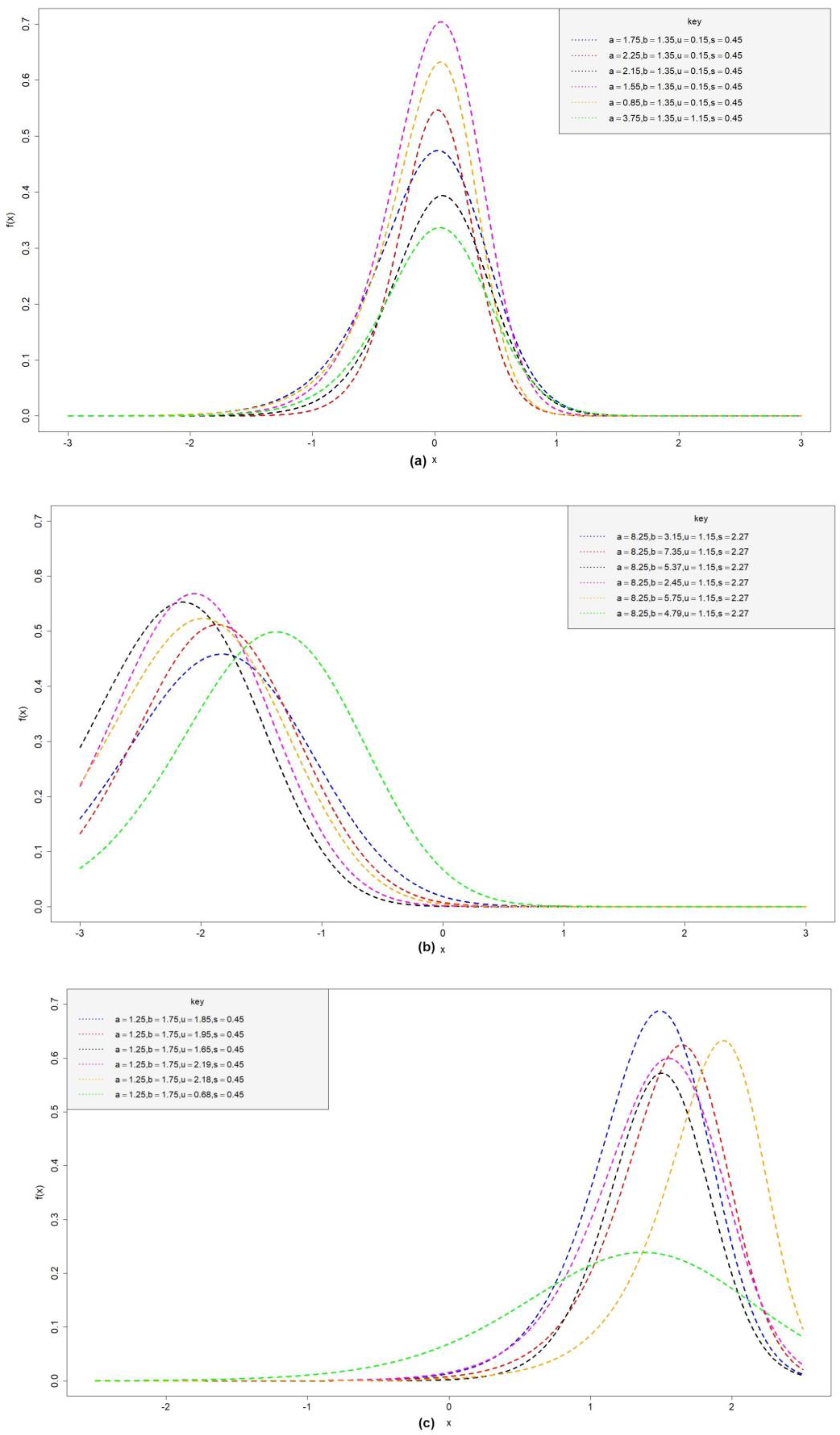
4. Development of Odd Beta Prime-Logistic Distribution

This section introduces a new PD called the odd beta prime-logistic (OBP-logistic) distribution, which is developed by adding two parameters of the LD defined in (4) to the OBP-G FPDs presented in (9). The cdf of OBP-logistic can be derived by inserting (3) in (7) as

$$\mathrm{F}\left(\mathrm{x}\right)=\frac{{\mathrm{B}}_{\frac{1}{\exp -\left(\frac{\mathrm{x}-\mathsf{\mu }}{\mathrm{s}}\right)}}\left(\mathrm{a},\mathrm{b}\right)}{\mathrm{B}\left(\mathrm{a},\mathrm{b}\right)}, \mathrm{x}\in ℝ.$$

(17)

The associated pdf of (17) is derived by inputting (3) and (4) into (9) to obtain

$$\mathrm{f}\left(\mathrm{x}\right)=\frac{1}{\mathrm{s}\mathrm{B}\left(\mathrm{a},\mathrm{b}\right)}\frac{{\left[\frac{1}{\exp -\left(\frac{\mathrm{x}-\mathsf{\mu }}{\mathrm{s}}\right)}\right]}^{\mathrm{a}}}{{\left[1+\frac{1}{\exp -\left(\frac{\mathrm{x}-\mathsf{\mu }}{\mathrm{s}}\right)}\right]}^{\mathrm{a}+\mathrm{b}}}, \mathrm{x}\in ℝ,$$

(18)

where $\mathrm{a},\mathrm{b}>0$ are shape parameters, $\mathsf{\mu }\in ℝ$ is the location parameter and $\mathrm{s}>0$ is the scale parameter. Several potential shapes of the new OBP-logistic distribution are depicted in Figure 1a–c. The different shapes of this PD include symmetric (a), positive-skewed (b), and negative-skewed (c).

The survival function of the OBP-logistic is expressed by

$$\mathrm{S}\left(\mathrm{x}\right)=1-\frac{{\mathrm{B}}_{\frac{1}{\exp -\left(\frac{\mathrm{x}-\mathsf{\mu }}{\mathrm{s}}\right)}}\left(\mathrm{a},\mathrm{b}\right)}{\mathrm{B}\left(\mathrm{a},\mathrm{b}\right)}, \mathrm{x}\in ℝ, \mathrm{a},\mathrm{b}>0.$$

(19)

The hazard rate of the OBP-logistic is defined as

$$\mathrm{h}\left(\mathrm{x}\right)=\frac{{\left[\frac{1}{\exp -\left(\frac{\mathrm{x}-\mathsf{\mu }}{\mathrm{s}}\right)}\right]}^{\mathrm{a}}}{\mathrm{s}\left[1+\frac{1}{\exp -\left(\frac{\mathrm{x}-\mathsf{\mu }}{\mathrm{s}}\right)}\right]\left[\mathrm{B}\left(\mathrm{a},\mathrm{b}\right)-{\mathrm{B}}_{\frac{1}{\exp -\left(\frac{\mathrm{x}-\mathsf{\mu }}{\mathrm{s}}\right)}}\left(\mathrm{a},\mathrm{b}\right)\right]}, \mathrm{x}\in ℝ, \mathrm{a},\mathrm{b}>0.$$

(20)

Figure 2a,b display some possible shapes of the hazard rate for the OBP-logistic model. As observed from the figure, the hazard rate of this PD can assume flexible shapes, for some chosen parameter values. In addition, it is observed from Figure 2a,b that the hazard rate of the OBP-logistic model indicates decreasing (a) and increasing (b) shapes.

5. Statistical Features of OBP-Logistic Distribution

This section covers derivations for various statistical features of the OBP-logistic model.

5.1. Moments

This subsection provides the $\mathrm{rth}$ moment for the OBP-logistic distribution.

If we suppose that X follows the OBP-logistic distribution, the $\mathrm{rth}$ moment of X is expressed by

$$\mathrm{E}\left({\mathrm{X}}^{\mathrm{r}}\right)={\displaystyle \underset{-\infty }{\overset{\infty }{\int }}{\mathrm{x}}^{\mathrm{r}}\mathrm{f}(\mathrm{x})\mathrm{d}\mathrm{x}},$$

(21)

where $\mathrm{f}(\mathrm{x})$ is defined in (16), and using (16) and (21), we can obtain

$$\mathrm{E}\left({\mathrm{X}}^{\mathrm{r}}\right)={\displaystyle \sum _{\mathrm{j},\mathrm{k}=0}^{\infty }{\Lambda }_{\mathrm{j},\mathrm{k}}}{\displaystyle \underset{-\infty }{\overset{\infty }{\int }}{\mathrm{x}}^{\mathrm{r}}\mathrm{q}\left(\mathrm{x}\right) {\left(\mathrm{Q}\left(\mathrm{x}\right)\right)}^{\mathrm{a}+\mathrm{j}+\mathrm{k}-1}\mathrm{d}\mathrm{x}}.$$

(22)

By substituting (3) and (4), the moments in (22), we have

$$\mathrm{E}\left({\mathrm{X}}^{\mathrm{r}}\right)={\displaystyle \sum _{\mathrm{j},\mathrm{k}=0}^{\infty }\frac{{\Lambda }_{\mathrm{j},\mathrm{k}}}{\mathrm{S}}}{\displaystyle \underset{-\infty }{\overset{\infty }{\int }}{\mathrm{x}}^{\mathrm{r}} \frac{\exp -\left(\frac{\mathrm{x}-\mathsf{\mu }}{\mathrm{s}}\right)}{{\left(1+\exp -\left(\frac{\mathrm{x}-\mathsf{\mu }}{\mathrm{s}}\right)\right)}^{\mathrm{a}+\mathrm{j}+\mathrm{k}+1}}\mathrm{d}\mathrm{x}}.$$

(23)

We can set

$$\mathrm{m}=\frac{1}{1+\exp -\left(\frac{\mathrm{x}-\mathsf{\mu }}{\mathrm{s}}\right)}, \mathrm{so} \mathrm{that} \mathrm{d}\mathrm{x}= \frac{\mathrm{s}}{\mathrm{m}\left(1-\mathrm{m}\right)} \mathrm{d}\mathrm{m}.$$

(24)

By inserting (24) in (23), we obtain

$$\mathrm{E}\left({\mathrm{X}}^{\mathrm{r}}\right)={\displaystyle \sum _{\mathrm{j},\mathrm{k}=0}^{\infty }{\Lambda }_{\mathrm{j},\mathrm{k}}}{\displaystyle \underset{0}{\overset{1}{\int }}{\left[\mathsf{\mu }-\mathrm{s}\log \left(\frac{1-\mathrm{m}}{\mathrm{m}}\right)\right]}^{\mathrm{r}}\left(1-\mathrm{m}\right){\left(\mathrm{m}\right)}^{\mathrm{a}+\mathrm{j}+\mathrm{k}}\mathrm{d}\mathrm{m}.}$$

By setting $\mathrm{r}=1$, we obtain

$$\begin{array}{l}\mathrm{E}\left(\mathrm{x}\right)={\displaystyle \sum _{\mathrm{j},\mathrm{k}=0}^{\infty }{\Lambda }_{\mathrm{j},\mathrm{k}}}\left\{\mathsf{\mu }\left[{\displaystyle \underset{0}{\overset{1}{\int }}{\left(1-\mathrm{m}\right)}^{2-1}{\left(\mathrm{m}\right)}^{\mathrm{a}+\mathrm{j}+\mathrm{k}+1-1}\mathrm{d}\mathrm{m}}\right]\right\}-\\ {\displaystyle \sum _{\mathrm{j},\mathrm{k}=0}^{\infty }{\Lambda }_{\mathrm{j},\mathrm{k}}} \left\{\mathrm{s}\left[{\displaystyle \underset{0}{\overset{1}{\int }}\log \left(1-\mathrm{m}\right)\left(1-\mathrm{m}\right){\left(\mathrm{m}\right)}^{\mathrm{a}+\mathrm{j}+\mathrm{k}}\mathrm{d}\mathrm{m}-{\displaystyle \underset{0}{\overset{1}{\int }}\log \left(\mathrm{m}\right)\left(1-\mathrm{m}\right){\left(\mathrm{m}\right)}^{\mathrm{a}+\mathrm{j}+\mathrm{k}}\mathrm{d}\mathrm{m}}}\right]\right\},\end{array}$$

(25)

where $\mathrm{E}\left(\mathrm{X}\right)$ is the mean for the OBP-logistic distribution.

Therefore, $\log (\mathrm{m})={\displaystyle \sum _{\mathrm{c}=1}^{\infty }\frac{{(-1)}^{\mathrm{c}+1}{\left(\mathrm{w}-1\right)}^{\mathrm{c}}}{\mathrm{c}}}$ for $0<\mathrm{m}\le 2$ and $\log (1-\mathrm{m})=\left(-{\displaystyle \sum _{\mathrm{c}=1}^{\infty }\frac{{(-1)}^{\mathrm{c}}{\left(-\mathrm{m}\right)}^{\mathrm{c}}}{\mathrm{c}}}\right)$ for $\left|\mathrm{m}\right|<1.$ This form of expansion expressed in (25) has been studied in [67] in Theorem 3.5.

Thus, Equation (25) gives

$$\begin{array}{ll}\mathrm{E}\left(\mathrm{X}\right)=& \mathsf{\mu }\mathrm{B}\left(2 , \mathrm{a}+\mathrm{j}+\mathrm{k}+1\right){\displaystyle \sum _{\mathrm{j},\mathrm{k}=0}^{\infty }{\Lambda }_{\mathrm{j},\mathrm{k}}}-\\ & \mathrm{s}\left\{{\displaystyle \sum _{\mathrm{c}=1}^{\infty }\frac{{(-1)}^{2\mathrm{c}}}{\mathrm{c}}}\left(\mathrm{B}\left(\mathrm{c}+1 , \mathrm{a}+\mathrm{j}+\mathrm{k}+1\right) , \mathrm{B}\left(2 , \mathrm{a}+\mathrm{j}+\mathrm{k}+\mathrm{c}+1\right)\right)\right\}.\end{array}$$

(26)

This is the mean of the OBP-logistic distribution.

5.2. Moment-Generating Function (mgf)

The derivation of the mgf of OBP-logistic distribution in terms of the mixture representation defined in (16) is provided in this subsection.

If we assume that RV X follows the OBP-logistic distribution, the mgf of X is given by

$${\mathrm{M}}_{\mathrm{x}}\left(\mathrm{t}\right)=\mathrm{E}\left(\exp \left(\mathrm{t}\mathrm{X}\right)\right)={\displaystyle \underset{-\infty }{\overset{\infty }{\int }}\exp \left(\mathrm{t}\mathrm{x}\right)\mathrm{f}(\mathrm{x})\mathrm{d}\mathrm{x}},$$

(27)

provided that this expectation exists for $\mathrm{t}$ in some neighborhood of 0.

Using (16) and (27), we obtain

$${\mathrm{M}}_{\mathrm{x}}\left(\mathrm{t}\right)={\displaystyle \sum _{\mathrm{j},\mathrm{k}=0}^{\infty }{\Lambda }_{\mathrm{j},\mathrm{k}}}{\displaystyle \underset{-\infty }{\overset{\infty }{\int }}\exp \left(\mathrm{t}\mathrm{x}\right) \mathrm{q}\left(\mathrm{x}\right) {\left(\mathrm{Q}\left(\mathrm{x}\right)\right)}^{\mathrm{a}+\mathrm{j}+\mathrm{k}-1}\mathrm{d}\mathrm{x}}.$$

(28)

Substituting (3) and (4) in (28), we obtain

$${\mathrm{M}}_{\mathrm{x}}\left(\mathrm{t}\right)={\displaystyle \sum _{\mathrm{j},\mathrm{k}=0}^{\infty }\frac{{\Lambda }_{\mathrm{j},\mathrm{k}}}{\mathrm{s}}}{\displaystyle \underset{-\infty }{\overset{\infty }{\int }}\exp \left(\mathrm{t}\mathrm{x}\right) \frac{\exp -\left(\frac{\mathrm{x}-\mathsf{\mu }}{\mathrm{s}}\right)}{{\left(1+\exp -\left(\frac{\mathrm{x}-\mathsf{\mu }}{\mathrm{s}}\right)\right)}^{\mathrm{a}+\mathrm{j}+\mathrm{k}+1}}\mathrm{d}\mathrm{x}}.$$

(29)

With the following equation,

$$\mathrm{m}=\frac{1}{1+\exp -\left(\frac{\mathrm{x}-\mathsf{\mu }}{\mathrm{s}}\right)}, \mathrm{we} \mathrm{obtain} \mathrm{d}\mathrm{x}= \frac{\mathrm{s}{\left(1+\exp -\left(\frac{\mathrm{x}-\mathsf{\mu }}{\mathrm{s}}\right)\right)}^2}{\exp -\left(\frac{\mathrm{x}-\mathsf{\mu }}{\mathrm{s}}\right)} \mathrm{d}\mathrm{m}.$$

(30)

Inserting (30) in (29), we have

$${\mathrm{M}}_{\mathrm{x}}\left(\mathrm{t}\right)=\exp \left(\mathrm{m}\mathrm{t}\right){\displaystyle \sum _{\mathrm{j},\mathrm{k}=0}^{\infty }{\Lambda }_{\mathrm{j},\mathrm{k}}}{\displaystyle \underset{0}{\overset{1}{\int }}{\mathrm{m}}^{\mathrm{a}+\mathrm{j}+\mathrm{k}+\mathrm{s}\mathrm{t}-1}{\left(1-\mathrm{m}\right)}^{1-\mathrm{s}\mathrm{t}-1}\mathrm{d}\mathrm{m}.}$$

(31)

After simplifications, we obtained the mgf of the OBP-logistic distribution as

$${\mathrm{M}}_{\mathrm{x}}\left(\mathrm{t}\right)=\exp \left(\mathrm{m}\mathrm{t}\right){\displaystyle \sum _{\mathrm{j},\mathrm{k}=0}^{\infty }{\Lambda }_{\mathrm{j},\mathrm{k}}} \mathrm{B}\left(\mathrm{a}+\mathrm{j}+\mathrm{k}+\mathrm{s}\mathrm{t} , 1-\mathrm{s}\mathrm{t}\right).$$

(32)

5.3. Information-Generating Function (IGF)

In information theory and statistics, the IGF has been utilized to generate some important information quantities, such as Kullback–Leibler divergence and Shannon entropy. It has been widely applied in physics and chemistry to analyze the atomic structure of a given phenomenon or system. This subsection provides the derivation of the IGF of OBP-logistic distribution.

The IGF of the RV X is given as

$${\mathrm{I}}_{\mathsf{\gamma }}(\mathrm{x})={\displaystyle \underset{-\infty }{\overset{\infty }{\int }}{\mathrm{f}}^{\mathsf{\gamma }}(\mathrm{x})\mathrm{d}\mathrm{x}}, \mathrm{for} \mathsf{\gamma }>0,$$

(33)

when the integral is finite.

$\mathrm{f}$ is defined in (18). Hereafter, the integrand ${\mathrm{f}}^{\mathsf{\gamma }}(\mathrm{x})$ in (33) can be given by

$${\mathrm{f}}^{\mathsf{\gamma }}\left(\mathrm{x}\right)=\frac{1}{{\left\{\mathrm{s}\mathrm{B}\left(\mathrm{a},\mathrm{b}\right)\right\}}^{\mathsf{\gamma }}}\frac{{\left[1/\exp -\left(\frac{\mathrm{x}-\mathsf{\mu }}{\mathrm{s}}\right)\right]}^{\mathrm{a}·\mathsf{\gamma }}}{{\left[1+1/\exp -\left(\frac{\mathrm{x}-\mathsf{\mu }}{\mathrm{s}}\right)\right]}^{(\mathrm{a}+\mathrm{b})·\mathsf{\gamma }}}.$$

(34)

Using (23), the integrand in (34) is

$${\mathrm{f}}^{\mathsf{\gamma }}\left(\mathrm{x}\right)={\left\{\mathrm{s}\mathrm{B}\left(\mathrm{a},\mathrm{b}\right)\right\}}^{\mathsf{\gamma }}\frac{{\left(\frac{1}{\mathrm{w}}-1\right)}^{\mathrm{a}\mathsf{\gamma }}}{{\left(\frac{1}{\mathrm{w}}\right)}^{(\mathrm{a}+\mathrm{b})\mathsf{\gamma }}},$$

(35)

where $\mathrm{w}=\frac{1}{1+\frac{1}{\exp -\left(\frac{\mathrm{x}-\mathsf{\mu }}{\mathrm{s}}\right)}}.$

$$\mathrm{By} \mathrm{setting} \mathrm{d}\mathrm{x}=-\frac{{\left(\frac{1}{\mathrm{w}}\right)}^2}{\frac{1}{\mathrm{s}·\left(\frac{\mathrm{w}}{1-\mathrm{w}}\right)}}, \mathrm{we} \mathrm{can} \mathrm{obtain} \mathrm{d}\mathrm{w} =-\frac{\mathrm{s}\mathrm{d}\mathrm{w}}{\mathrm{w}(1-\mathrm{w})}.$$

(36)

By inputting (35) and (36) into (33), we have

$$\begin{array}{ll}{\mathrm{I}}_{\mathsf{\gamma }}(\mathrm{x})& =\frac{1}{{\left\{\mathrm{s}\mathrm{B}\left(\mathrm{a},\mathrm{b}\right)\right\}}^{\mathsf{\gamma }}}{\displaystyle \underset{0}{\overset{1}{\int }}\frac{{\left(\frac{1}{\mathrm{w}}-1\right)}^{\mathrm{a}\mathsf{\gamma }}}{{\left(\frac{1}{\mathrm{w}}\right)}^{(\mathrm{a}+\mathrm{b})\mathsf{\gamma }}}}\frac{\mathrm{s}\mathrm{d}\mathrm{w}}{\mathrm{w}(1-\mathrm{w})}\\ & =\frac{\mathrm{s}}{{\left\{\mathrm{s}\mathrm{B}\left(\mathrm{a},\mathrm{b}\right)\right\}}^{\mathsf{\gamma }}}\mathrm{B}\left(\mathsf{\gamma }\mathrm{b} , \mathsf{\gamma }\mathrm{a}\right).\end{array}$$

(37)

This gives the igf of the OBP-logistic distribution.

5.4. Quantile Function

One can suppose the RV X follows the OBP-logistic distribution with cdf (17). Then, the quantile function (QF) of the OBP-logistic model is derived by inverting (17) as follows:

$$\mathrm{F}\left(\mathrm{x}\right)=\frac{ {\mathrm{B}}_{\frac{\mathrm{Q}\left(\mathrm{x}\right)}{1-\mathrm{Q}\left(\mathrm{x}\right)}}\left(\mathrm{a},\mathrm{b}\right)}{\mathrm{B}\left(\mathrm{a},\mathrm{b}\right)}=\mathrm{I}\left(\frac{\mathrm{Q}\left(\mathrm{x}\right)}{1-\mathrm{Q}\left(\mathrm{x}\right)} ; \mathrm{a},\mathrm{b}\right).$$

(38)

The QF of the baseline cdf is computed by inverting (38) as

$$\frac{\mathrm{Q}\left(\mathrm{x}\right)}{1-\mathrm{Q}\left(\mathrm{x}\right)}={\mathrm{I}}^{-1}\left(\mathrm{u} ; \mathrm{a},\mathrm{b}\right).$$

Then, we can obtain

$$\mathrm{Q}\left(\mathrm{x}\right)\left[1+{\mathrm{I}}^{-1}\left(\mathrm{u} ; \mathrm{a},\mathrm{b}\right)\right]={\mathrm{I}}^{-1}\left(\mathrm{u} ; \mathrm{a},\mathrm{b}\right).$$

Therefore,

$$\mathrm{Q}\left(\mathrm{x}\right)=\frac{{\mathrm{I}}^{-1}\left(\mathrm{u} ; \mathrm{a},\mathrm{b}\right)}{1+{\mathrm{I}}^{-1}\left(\mathrm{u} ; \mathrm{a},\mathrm{b}\right)},$$

(39)

which is the QF of the baseline model, where $\mathrm{u}$ is the uniform random variable in the interval (0,1). The QF of the OBP-logistic model is obtained by inserting (3) in (39) as

$$\frac{1}{1+\exp -\left(\frac{\mathrm{x}-\mathsf{\mu }}{\mathrm{s}}\right)}=\mathrm{K},$$

where $\mathrm{K}=\frac{{\mathrm{I}}^{-1}\left(\mathrm{u} ; \mathrm{a},\mathrm{b}\right)}{1+{\mathrm{I}}^{-1}\left(\mathrm{u} ; \mathrm{a},\mathrm{b}\right)}.$

We can simplify (40) as

$$\mathrm{K}\left(1+\exp -\left(\frac{\mathrm{x}-\mathsf{\mu }}{\mathrm{s}}\right)\right)=1,$$

where $\mathrm{x}-\mathrm{u}=-\mathrm{s}\log \left(\frac{1-\mathrm{K}}{\mathrm{K}}\right).$

Hence, the QF of OBP-logistic model is

$$\mathrm{x}=\mathrm{u}-\mathrm{s}\log \left(\frac{1-\mathrm{K}}{\mathrm{K}}\right).$$

(40)

5.5. Stress–Strength

Here, we present the formulation of the stress–strength function of the OBP-logistic distribution. The stress–strength function is used to assess the reliability of a product exposed to variant stress [68].

If we suppose that X₁ and X₂ are two independent RVs with the OBP-logistic model with $\mathrm{a},\mathrm{b},\mathsf{\mu },\mathrm{s}$ parameters, then the stress–strength function of the OBP-logistic model is expressed by

$$\mathrm{R}=\mathrm{P}\left({\mathrm{X}}_2<{\mathrm{X}}_1\right)={\displaystyle \underset{-\infty }{\overset{\infty }{\int }}{\displaystyle \underset{-\infty }{\overset{{\mathrm{x}}_1}{\int }}\mathrm{f}\left({\mathrm{x}}_1;{\mathrm{a}}_1,\mathrm{b},\mathsf{\mu },\mathrm{s}\right)}}\mathrm{f}\left({\mathrm{x}}_2;{\mathrm{a}}_2,\mathrm{b},\mathsf{\mu },\mathrm{s}\right)\mathrm{d}{\mathrm{x}}_1\mathrm{d}{\mathrm{x}}_2.$$

(41)

where $\mathrm{R}=\mathrm{P}\left({\mathrm{X}}_2<{\mathrm{X}}_1\right)$ is the failure that occurs when the applied stress exceeds the system’s strength; $\mathrm{f}\left({\mathrm{x}}_1;{\mathrm{a}}_1,\mathrm{b},\mathsf{\mu },\mathrm{s}\right)$ and $\mathrm{F}\left({\mathrm{x}}_1;{\mathrm{a}}_2,\mathrm{b},\mathsf{\mu },\mathrm{s}\right)$ are the pdf and cdf of the OBP-logistic distribution. The integrand in (41) can be expressed as

$$\mathrm{R}={\displaystyle \underset{-\infty }{\overset{\infty }{\int }}\mathrm{f}\left({\mathrm{x}}_1;{\mathrm{a}}_1,\mathrm{b},\mathsf{\mu },\mathrm{s}\right)\mathrm{F}\left({\mathrm{x}}_1;{\mathrm{a}}_2,\mathrm{b},\mathsf{\mu },\mathrm{s}\right)}\mathrm{d}{\mathrm{x}}_1.$$

(42)

As given in [69], the cdf of the Beta function can be expanded as

$${\mathrm{I}}_{\mathrm{z}}(\mathrm{a},\mathrm{b})=\frac{{\mathrm{z}}^{\mathrm{a}}}{\mathrm{B}\left(\mathrm{a},\mathrm{b}\right)}{\displaystyle \sum _{\mathrm{i}=0}^{\infty }\frac{{\left(1-\mathrm{b}\right)}_{\mathrm{i}}}{{\left(\mathrm{a}+\mathrm{i}\right)}_{\mathrm{i}}!} }{\mathrm{z}}^{\mathrm{i}}.$$

(43)

Inserting (43) in (42), we obtain

$$\begin{array}{l}\mathrm{f}\left({\mathrm{x}}_1;{\mathrm{a}}_1,\mathrm{b},\mathsf{\mu },\mathrm{s}\right)\mathrm{F}\left({\mathrm{x}}_1;{\mathrm{a}}_2,\mathrm{b},\mathsf{\mu },\mathrm{s}\right)=\mathrm{f}\left({\mathrm{x}}_1;{\mathrm{a}}_1,\mathrm{b},\mathsf{\mu },\mathrm{s}\right)\times \\ \frac{{\left[\frac{1}{\exp -\left(\frac{\mathrm{x}-\mathsf{\mu }}{\mathrm{s}}\right)}\right]}^{{\mathrm{a}}_2}}{\mathrm{B}\left({\mathrm{a}}_2,\mathrm{b}\right)}{\displaystyle \sum _{\mathrm{i}=0}^{\infty }\frac{{\left(1-\mathrm{b}\right)}_{\mathrm{i}}}{{\left({\mathrm{a}}_2+\mathrm{i}\right)}_{\mathrm{i}}!}}{\left[\frac{1}{\exp -\left(\frac{\mathrm{x}-\mathsf{\mu }}{\mathrm{s}}\right)}\right]}^{\mathrm{i}}.\end{array}$$

(44)

For simplicity, (44) can be expressed as

$$\mathrm{f}\left({\mathrm{x}}_1;{\mathrm{a}}_1,\mathrm{b},\mathsf{\mu },\mathrm{s}\right)\mathrm{F}\left({\mathrm{x}}_1;{\mathrm{a}}_2,\mathrm{b},\mathsf{\mu },\mathrm{s}\right)=\Psi \times \mathrm{f}\left({\mathrm{x}}_1;{\mathrm{a}}_1,\mathrm{b},\mathsf{\mu },\mathrm{s}\right){{\displaystyle \sum _{\mathrm{i}=0}^{\infty }\left[\frac{1}{\exp -\left(\frac{\mathrm{x}-\mathsf{\mu }}{\mathrm{s}}\right)}\right]}}^{{\mathrm{a}}_2+\mathrm{i}},$$

(45)

where $\Psi =\frac{{\left(1-\mathrm{b}\right)}_{\mathrm{i}}}{\mathrm{B}\left({\mathrm{a}}_2,\mathrm{b}\right){\left({\mathrm{a}}_2+\mathrm{i}\right)}_{\mathrm{i}}!}.$

By inserting (45) in (41), we obtain

$$\mathrm{R}=\Psi \times \Omega {\displaystyle \underset{-\infty }{\overset{\infty }{\int }}\frac{{\left[\frac{1}{\exp -\left(\frac{\mathrm{x}-\mathsf{\mu }}{\mathrm{s}}\right)}\right]}^{{\mathrm{a}}_1+{\mathrm{a}}_2+\mathrm{i}}}{{\left[1+\left[\frac{1}{\exp -\left(\frac{\mathrm{x}-\mathsf{\mu }}{\mathrm{s}}\right)}\right]\right]}^{{\mathrm{a}}_1+\mathrm{b}}}}\mathrm{d}{\mathrm{x}}_1,$$

(46)

where $\Omega =\frac{1}{\mathrm{s}\mathrm{B}({\mathrm{a}}_1,\mathrm{b})}.$

When $\mathrm{y}=\frac{1}{\exp -\left(\frac{\mathrm{x}-\mathsf{\mu }}{\mathrm{s}}\right)},$ we can obtain the following equation:

$$\mathrm{d}{\mathrm{x}}_1=\mathrm{s}\times \exp -\left(\frac{\mathrm{x}-\mathsf{\mu }}{\mathrm{s}}\right).$$

(47)

Inserting (47) into (46), we have

$$\mathrm{R}=\Psi \times \Omega \times \mathrm{s}{\displaystyle \underset{-\infty }{\overset{\infty }{\int }}\frac{{\mathrm{y}}^{{\mathrm{a}}_1+{\mathrm{a}}_2+\mathrm{i}-1}}{{\left(1+\mathrm{y}\right)}^{{\mathrm{a}}_1+\mathrm{b}}}} \mathrm{d}\mathrm{y}.$$

(48)

After simplifications, the stress–strength function of the OBP-logistic model is

$$\mathrm{R}=\frac{1}{\mathrm{B}({\mathrm{a}}_1,\mathrm{b})\mathrm{B}({\mathrm{a}}_2,\mathrm{b})}{\displaystyle \sum _{\mathrm{i}=0}^{\infty }\frac{{\left(1-\mathrm{b}\right)}_{\mathrm{i}}}{{\left({\mathrm{a}}_2+\mathrm{i}\right)}_{\mathrm{i}}!}} \times \mathrm{B}\left({\mathrm{a}}_1+{\mathrm{a}}_2+\mathrm{i} , \mathrm{b}-{\mathrm{a}}_2-\mathrm{i}\right).$$

(49)

5.6. Order Statistics

Here, we derive the order statistics of the OBP-logistic. If we assume that the RV ${\mathrm{X}}_{1:\mathrm{n}},{\mathrm{X}}_{2:\mathrm{n}},\dots ,{\mathrm{X}}_{\mathrm{n}:\mathrm{n}}$ follows the OBP-logistic model and ${\mathrm{X}}_{1:\mathrm{n}}<{\mathrm{X}}_{2:\mathrm{n}}<\dots <{\mathrm{X}}_{\mathrm{n}:\mathrm{n}}$ is a set of RVs of $\mathrm{n}$ order, then the distribution of the $\mathrm{i}\mathrm{t}\mathrm{h}$ order statistics is

$${\mathrm{F}}_{\mathrm{i}:\mathrm{n}}\left(\mathrm{x}\right)=\frac{\mathrm{n}!}{\left(\mathrm{i}-1\right)!\left(\mathrm{n}-\mathrm{i}\right)!}{\left[\mathrm{F}\left(\mathrm{x}\right)\right]}^{\mathrm{i}-1}{\left[1-\mathrm{F}\left(\mathrm{x}\right)\right]}^{\mathrm{n}-\mathrm{i}}.$$

(50)

$${\mathrm{F}}_{\mathrm{i}:\mathrm{n}}\left(\mathrm{x}\right)=\frac{\mathrm{n}!\mathrm{f}\left(\mathrm{x}\right)}{\left(\mathrm{i}-1\right)!\left(\mathrm{n}-\mathrm{i}\right)!}{\displaystyle \sum _{\mathrm{j}=0}^{(\mathrm{n}-\mathrm{i})}{\left(-1\right)}^{\mathrm{j}}\left(\begin{array}{c}\mathrm{n}-\mathrm{i}\\ \mathrm{j}\end{array}\right)}{\mathrm{F}}_{\left(\mathrm{x}\right)}^{\mathrm{i}+\mathrm{j}-1},$$

(51)

where $\mathrm{f}$ and $\mathrm{F}$ are the pdf and cdf of the OBP-logistic model. Now, (51) can be expressed as

$${\mathrm{F}}_{\mathrm{i}:\mathrm{n}}\left(\mathrm{x}\right)=\frac{\mathrm{n}!\mathrm{f}\left(\mathrm{x}\right)}{\left(\mathrm{i}-1\right)!\left(\mathrm{n}-\mathrm{i}\right)!}{\displaystyle \sum _{\mathrm{j}=0}^{(\mathrm{n}-\mathrm{i})}{\left(-1\right)}^{\mathrm{j}}\left(\begin{array}{c}\mathrm{n}-\mathrm{i}\\ \mathrm{j}\end{array}\right)}\times {\displaystyle \sum _{\mathrm{k},\mathrm{m}=0}^{\infty }{\left(-1\right)}^{\mathrm{k}+\mathrm{m}}\left(\begin{array}{c}\mathrm{i}+\mathrm{j}-1\\ \mathrm{k}\end{array}\right)}\left(\begin{array}{l}\mathrm{k}\\ \mathrm{m}\end{array}\right){\mathrm{F}}_{\left(\mathrm{x}\right)}^{\mathrm{m}},$$

(52)

$${\mathrm{I}}_{\mathrm{x}}(\mathrm{a},\mathrm{b})=\frac{{\mathrm{x}}^{\mathrm{a}}}{\mathrm{B}\left(\mathrm{a},\mathrm{b}\right)}{\displaystyle \sum _{\mathrm{w}=0}^{\infty }\frac{{\left(1-\mathrm{b}\right)}_{\mathrm{w}}}{{\left(\mathrm{a}+\mathrm{w}\right)}_{\mathrm{w}\mathrm{i}}!} }{\mathrm{x}}^{\mathrm{w}}.$$

(53)

Inserting (53) into (52), we have

$${\mathrm{F}}_{\mathrm{i}:\mathrm{n}}\left(\mathrm{x}\right)=\mathrm{f}\left(\mathrm{x}\right){\displaystyle \sum _{\mathrm{j}=0}^{(\mathrm{n}-\mathrm{i})}{{\displaystyle \sum _{\mathrm{k},\mathrm{m}=0}^{\infty }{\Psi }_{\mathrm{j},\mathrm{k},\mathrm{m}}\left[\frac{{\left(\frac{1}{\exp -\left(\frac{\mathrm{x}-\mathsf{\mu }}{\mathrm{s}}\right)}\right)}^{\mathrm{a}}}{\mathrm{B}\left(\mathrm{a},\mathrm{b}\right)}{\displaystyle \sum _{\mathrm{w}=0}^{\infty }\frac{{\left(1-\mathrm{b}\right)}_{\mathrm{w}}}{{\left(\mathrm{a}+\mathrm{w}\right)}_{\mathrm{w}}{}_{\mathrm{i}}!}\times {\left(\frac{1}{\exp -\left(\frac{\mathrm{x}-\mathsf{\mu }}{\mathrm{s}}\right)}\right)}^{\mathrm{w}}}\right]}}^{\mathrm{m}}.}$$

(54)

$$\begin{array}{ll}{\mathrm{F}}_{\mathrm{i}:\mathrm{n}}\left(\mathrm{x}\right)=& {\displaystyle \sum _{{\mathrm{w}}_1}^{\infty }\dots {\displaystyle \sum _{\mathrm{m}=0}^{\infty }\left[\frac{{\left(1-\mathrm{b}\right)}_{{\mathrm{w}}_1}\dots {\left(1-\mathrm{b}\right)}_{{\mathrm{w}}_{\mathrm{m}}}\times {\left(\frac{1}{\exp -\left(\frac{\mathrm{x}-\mathsf{\mu }}{\mathrm{s}}\right)}\right)}^{\mathrm{a}+\mathrm{a}\mathrm{m}+{\mathrm{w}}_1+\dots +{\mathrm{w}}_{\mathrm{m}}-1}}{{\left[\mathrm{B}\left(\mathrm{a},\mathrm{b}\right)\right]}^{\mathrm{m}}\times \left(\mathrm{a}+{\mathrm{w}}_1\right)\dots \left(\mathrm{a}+{\mathrm{w}}_{\mathrm{m}}\right){\mathrm{w}}_1!\dots {\mathrm{w}}_{\mathrm{m}}!}\right]}\times }\\ & \frac{1}{\mathrm{s}\mathrm{B}\left(\mathrm{a},\mathrm{b}\right)}{\left[1+\frac{1}{\exp -\left(\frac{\mathrm{x}-\mathsf{\mu }}{\mathrm{s}}\right)}\right]}^{-(\mathrm{a}+\mathrm{b})}{\displaystyle \sum _{\mathrm{j}=0}^{(\mathrm{n}-\mathrm{i})}{\displaystyle \sum _{\mathrm{k},\mathrm{m}=0}^{\infty }{\Psi }_{\mathrm{j},\mathrm{k},\mathrm{m}}}.}\end{array}$$

(55)

Applying the Kampé de Fériet series [70], (54) can be expressed as

$$\begin{array}{l}{\mathrm{F}}_{\mathrm{i}:\mathrm{n}}\left(\mathrm{x}\right)=\frac{{\left(\frac{1}{\exp -\left(\frac{\mathrm{x}-\mathsf{\mu }}{\mathrm{s}}\right)}\right)}^{\mathrm{a}\left(1+\mathrm{m}\right)-1}}{\mathrm{s}\mathrm{B}{\left(\mathrm{a},\mathrm{b}\right)}^{1+\mathrm{m}}{\left[1+\frac{1}{\exp -\left(\frac{\mathrm{x}-\mathsf{\mu }}{\mathrm{s}}\right)}\right]}^{\mathrm{a}+\mathrm{b}}}\times {\mathrm{a}}^{-\mathrm{m}}{\displaystyle \sum _{\mathrm{j}=0}^{(\mathrm{n}-\mathrm{i})}{\displaystyle \sum _{\mathrm{k},\mathrm{m}=0}^{\infty }{\Psi }_{\mathrm{j},\mathrm{k},\mathrm{m}}}\times }\\ {\mathrm{F}}_{1:1}^{1:2}\left(\mathrm{a}\left(1+\mathrm{m}\right):\left(1-\mathrm{b},\mathrm{a}\right),\dots ,\left(1-\mathrm{b},\mathrm{a}\right),\left(\mathrm{b}+\mathrm{a}\left(1+\mathrm{m}\right)\right):\left(\mathrm{a}+1\right),\dots ,\left(\mathrm{a}+1\right),1,\dots ,1\right).\end{array}$$

(56)

This is the order statistics of the OBP-logistic model.

5.7. Entropies

In this subsection, two measures of variation in uncertainty that include the Rényi and $\mathrm{q}$ entropies are presented.

If we assume that X is a RV with pdf $\mathrm{f}$, the Rényi entropy [71] is expressed by

$${\mathrm{R}}_{\mathsf{\gamma }}(\mathrm{x})=\frac{1}{1-\mathsf{\gamma }}\log \left[{\displaystyle \underset{-\infty }{\overset{\infty }{\int }}{\mathrm{f}}^{\mathsf{\gamma }}(\mathrm{x})\mathrm{d}\mathrm{x}}\right], \mathsf{\gamma }>0, \mathsf{\gamma }\ne 1, \mathrm{x}\in ℝ,$$

(57)

where $\mathrm{f}$ is the pdf of the OBP-logistic distribution.

Using (37) and (57), we have

$${\mathrm{R}}_{\mathsf{\gamma }}(\mathrm{x})=\frac{1}{1-\mathsf{\gamma }}\log \left[\frac{\mathrm{s}}{{\left\{\mathrm{s}\mathrm{B}\left(\mathrm{a},\mathrm{b}\right)\right\}}^{\mathsf{\gamma }}}\mathrm{B}\left(\mathsf{\gamma }\mathrm{b} , \mathsf{\gamma }\mathrm{a}\right)\right].$$

(58)

The expression of the $\mathrm{q}$-entropy is given by

$${\mathrm{Q}}_{\mathsf{\gamma }}(\mathrm{x})=\frac{1}{1-\mathsf{\gamma }}\log \left[1-{\displaystyle \underset{-\infty }{\overset{\infty }{\int }}{\mathrm{f}}^{\mathsf{\gamma }}(\mathrm{x})\mathrm{d}\mathrm{x}}\right], \mathsf{\gamma }>0, \mathsf{\gamma }\ne 1, \mathrm{x}\in ℝ.$$

(59)

The $\mathrm{q}$-entropy is obtained by substituting (37) as

$${\mathrm{Q}}_{\mathsf{\gamma }}(\mathrm{x})=\frac{1}{1-\mathsf{\gamma }}\log \left[1-\left[\frac{\mathrm{s}}{{\left\{\mathrm{s}\mathrm{B}\left(\mathrm{a},\mathrm{b}\right)\right\}}^{\mathsf{\gamma }}}\mathrm{B}\left(\mathsf{\gamma }\mathrm{b} , \mathsf{\gamma }\mathrm{a}\right)\right]\right].$$

(60)

6. Maximum Likelihood Estimation

Here, we use the MLE method to develop estimators for estimating the parameters of the OBP-logistic model. If we assume that ${\mathrm{x}}_1,{\mathrm{x}}_2,\dots {\mathrm{x}}_{\mathrm{n}}$ are the possible outcomes of an experimental sample of size $(\mathrm{n})$ drawn from a OBP-logistic model with set of parameters $\Phi =\left(\mathrm{a},\mathrm{b},\mathsf{\mu },\mathrm{s}\right)$, then the likelihood function for the parameter vector $\Phi ={\left(\mathrm{a},\mathrm{b},\mathsf{\mu },\mathrm{s}\right)}^{\mathrm{T}}$ is given by

$$\mathrm{L}\left(\mathrm{x};\mathrm{a},\mathrm{b},\mathsf{\mu },\mathrm{s}\right)={\left\{\frac{\Gamma (\mathrm{a}+\mathrm{b})}{\mathrm{s}\Gamma (\mathrm{a})\Gamma (\mathrm{b})}\right\}}^{\mathrm{n}}{\displaystyle \prod _{\mathrm{i}=1}^{\mathrm{n}}\frac{{\left(\frac{1}{\exp -\left(\frac{\mathrm{x}-\mathsf{\mu }}{\mathrm{s}}\right)}\right)}^{\mathrm{a}}}{{\left(1+\frac{1}{\exp -\left(\frac{\mathrm{x}-\mathsf{\mu }}{\mathrm{s}}\right)}\right)}^{\mathrm{a}+\mathrm{b}}}},$$

(61)

where $\mathrm{B}\left(\mathrm{a},\mathrm{b}\right)=\frac{\Gamma (\mathrm{a})\Gamma (\mathrm{b})}{\Gamma (\mathrm{a}+\mathrm{b})}$ (see [72]).

Then, the log-likelihood function of (61) is

$$\begin{array}{ll}\mathcal{l}=\log \mathrm{L}\left(\mathrm{x};\mathrm{a},\mathrm{b},\mathsf{\mu },\mathrm{s}\right)=& \mathrm{n}\log \left(\Gamma (\mathrm{a}+\mathrm{b})\right)-\mathrm{n}\log \left(\mathrm{s}\right)-\mathrm{n}\log \left(\Gamma (\mathrm{a})\right)-\mathrm{n}\log \left(\Gamma (\mathrm{b})\right)\\ & +\mathrm{a}{\displaystyle \sum _{\mathrm{i}=1}^{\mathrm{n}}\log \left(\frac{1}{\exp -\left(\frac{{\mathrm{x}}_{\mathrm{i}}-\mathsf{\mu }}{\mathrm{s}}\right)}\right)}-\left(\mathrm{a}+\mathrm{b}\right){\displaystyle \sum _{\mathrm{i}=1}^{\mathrm{n}}\log \left(1+\frac{1}{\exp -\left(\frac{{\mathrm{x}}_{\mathrm{i}}-\mathsf{\mu }}{\mathrm{s}}\right)}\right)}.\end{array}$$

(62)

The ML estimates (MLEs) $\widehat{\Phi }$ of $\Phi$ are determined by maximizing (62). The components of the score vector with respect to $\mathrm{a},\mathrm{b},\mathsf{\mu }$ and $\mathrm{s}$ are

$$\frac{\partial \mathcal{l}}{\partial \mathrm{a}}=\mathrm{n}\psi (\mathrm{a}+\mathrm{b})-\mathrm{n}\psi (\mathrm{a})+{\displaystyle \sum _{\mathrm{i}=1}^{\mathrm{n}}\log \left(\frac{1}{\exp -\left(\frac{{\mathrm{x}}_{\mathrm{i}}-\mathsf{\mu }}{\mathrm{s}}\right)}\right)}-{\displaystyle \sum _{\mathrm{i}=1}^{\mathrm{n}}\log \left(1+\frac{1}{\exp -\left(\frac{{\mathrm{x}}_{\mathrm{i}}-\mathsf{\mu }}{\mathrm{s}}\right)}\right)},$$

(63)

$$\frac{\partial \mathcal{l}}{\partial \mathrm{b}}=\mathrm{n}\psi (\mathrm{a}+\mathrm{b})-\mathrm{n}\psi (\mathrm{b})-{\displaystyle \sum _{\mathrm{i}=1}^{\mathrm{n}}\log \left(1+\frac{1}{\exp -\left(\frac{{\mathrm{x}}_{\mathrm{i}}-\mathsf{\mu }}{\mathrm{s}}\right)}\right)},$$

(64)

$$\frac{\partial \mathcal{l}}{\partial \mathsf{\mu }}=-\frac{\mathrm{n}\mathrm{a}}{\mathrm{s}}+\frac{(\mathrm{a}+\mathrm{b})}{\mathrm{s}}{\displaystyle \sum _{\mathrm{i}=1}^{\mathrm{n}}\left[\frac{1}{1+\exp -\left(\frac{{\mathrm{x}}_{\mathrm{i}}-\mathsf{\mu }}{\mathrm{s}}\right)}\right]},$$

(65)

$$\frac{\partial \mathcal{l}}{\partial \mathrm{s}}=-\frac{\mathrm{n}}{\mathrm{s}}-\frac{\mathrm{a}}{{\mathrm{s}}^2}{\displaystyle \sum _{\mathrm{i}=1}^{\mathrm{n}}\left({\mathrm{x}}_{\mathrm{i}}-\mathsf{\mu }\right)}+\frac{(\mathrm{a}+\mathrm{b})}{{\mathrm{s}}^2}{\displaystyle \sum _{\mathrm{i}=1}^{\mathrm{n}}\left(\frac{\left({\mathrm{x}}_{\mathrm{i}}-\mathsf{\mu }\right)}{1+\exp -\left(\frac{{\mathrm{x}}_{\mathrm{i}}-\mathsf{\mu }}{\mathrm{s}}\right)}\right)},$$

(66)

where $\psi$ is the digamma function.

The estimators for the parameters can be obtained by setting (63)–(66) to zero. Although it is laborious to find the system’s solutions analytically, the R programming language [73] provides the numerical solutions of the system using iterative Newton–Raphson methods.

7. Monte Carlo Simulation Study

Here, we test the accuracy of the MLEs based on $\mathrm{n}$ random samples. Simulations are performed to study the behavior of the MLE for the OBP-logistic distribution. It is employed for maximizing (62). The number of simulation replicates is observed for $\mathrm{R}=1000$ times on different random samples of various sizes of $\mathrm{n}=50, 150, 300,\dots , 2050$. The average MLEs, biases, and mean square errors (MSEs) are obtained at each sample size based on the quantile function defined in (40). The average bias and MSE can be expressed as

$$\mathrm{Bias}=\frac{1}{\mathrm{R}}{\displaystyle \sum _{\mathrm{i}=1}^{\mathrm{R}}\left({\widehat{\Phi }}_{\mathrm{i}}-\Phi \right)},$$

(67)

$$\mathrm{MSE}=\frac{1}{\mathrm{R}}{{\displaystyle \sum _{\mathrm{i}=1}^{\mathrm{R}}\left({\widehat{\Phi }}_{\mathrm{i}}-\Phi \right)}}^2,$$

(68)

where $\Phi ={(\mathrm{a},\mathrm{b},\mathsf{\mu },\mathrm{s})}^{\mathrm{T}}.$

Table 1. Simulation results (MLE, bias, and MSE) for OBP-logistic distribution for several values.

		$\mathbf{Set} 1: \mathbf{a} = 0.5, \mathbf{b} = 1.5, \mathbf{\mu } = 0.75, \mathbf{s}=0.5$			Set 2: $\mathbf{a} = 0.35, \mathbf{b} = 1.7, \mathbf{\mu } = 1.2, \mathbf{s} = 0.2$
Parameter	n	Mean	Bias	MSE	Mean	Bias	MSE
$\widehat{\mathrm{a}}$	50	1.021639	0.421634	0.323464	0.376896	0.069939	0.051017
	150	0.783206	0.283205	0.159113	0.415324	0.154217	0.051843
	300	0.705664	0.205666	0.088489	0.387839	0.097845	0.026851
	750	0.632203	0.132208	0.053510	0.377562	0.070852	0.018937
	1050	0.579878	0.079871	0.024855	0.369832	0.059126	0.013711
	1550	0.534531	0.064537	0.016711	0.360532	0.047211	0.008374
	2050	0.511279	0.061279	0.015390	0.356891	0.036824	0.004921
$\widehat{\mathrm{b}}$	50	3.071120	2.051126	6.501042	2.757921	1.057934	8.337832
	150	2.335925	1.315927	4.281831	1.903067	0.203953	1.077834
	300	1.916825	0.896823	2.927313	1.815383	0.115848	0.662473
	750	1.853472	0.533476	1.630027	1.725902	0.025954	0.398832
	1050	1.801139	0.265113	0.727289	1.724942	0.290710	0.024529
	1550	1.795770	0.178776	0.410361	1.717291	0.004975	0.193952
	2050	1.628714	0.156718	0.363602	1.704701	0.002562	0.009541
$\widehat{\mathsf{\mu }}$	50	0.526858	−0.273106	0.104449	1.875402	0.780864	3.704327
	150	0.620049	−0.179951	0.060271	1.460174	0.208016	0.877854
	300	0.662551	−0.137446	0.039444	1.386421	0.072756	0.392853
	750	0.709550	−0.090441	0.023709	1.283419	0.049643	0.270834
	1050	0.715512	−0.074489	0.017091	1.247242	0.015953	0.174934
	1550	0.739470	−0.057208	0.010584	1.227641	0.010261	0.118342
	2050	0.757674	−0.042325	0.007179	1.207845	0.007834	0.111962
$\widehat{\mathrm{s}}$	50	0.657450	0.089643	0.010547	0.234628	0.012999	0.009617
	150	0.579762	0.019884	0.005913	0.238917	0.038921	0.005998
	300	0.546031	0.009546	0.001750	0.233610	0.023610	0.004892
	750	0.536545	0.006575	0.001147	0.229828	0.019721	0.003671
	1050	0.524567	0.004567	0.000756	0.222611	0.016963	0.002930
	1550	0.534541	0.003454	0.000471	0.218936	0.012953	0.002538
	2050	0.546522	0.002622	0.000242	0.204097	0.009618	0.001273

displays the simulation results for different parameter values. Accuracy is achieved as the estimates tend to be closer to their actual values when the $\mathrm{n}$ increases. At first, we generate 1000 random samples from the OBP-logistic distribution $(\mathrm{a},\mathrm{b},\mathsf{\mu },\mathrm{s})$ from different variations in the parameters $(\mathrm{a}=0.5, \mathrm{b}=1.5, \mathsf{\mu }=0.75, \mathrm{s}=0.5)$ for fixed sample sizes $\mathrm{n}=50, 150, 300,\dots , 2050$ and secondly, for different variations in the parameters $(\mathrm{a}=0.35, \mathrm{b}=1.7, \mathsf{\mu }=1.2, \mathrm{s}=0.2)$ for the fixed sample sizes $\mathrm{n}=50, 150, 300,\dots , 2050$.

In addition, the values of the error measures of the parameter estimates decrease when the $\mathrm{n}$ increases. Therefore, it is evident that the MLE approach generates consistent estimates in assessing the parameters of the OBP-logistic distribution for all possible parameter value selections. Table 1 also demonstrated that as $\mathrm{n}$ increases, the MSE for the estimators decreases.

8. Applications

This section illustrates the performance of the new OBP-logistic model against several competitive models using data from gas fiber (GF), carbon fiber (CF) and magnesium concentrations (MC). The fitting flexibility of the OBP-logistic distribution is measured by comparing it to the gamma generalized logistic (GGL) distribution [74], new modified exponential logistic (NMEL) distribution [75], gamma- logistic (GL) distribution [45], exponential modified Weibull logistic (EMWL) distribution [76], exponentiated Weibull logistic (EWL) distribution [77], and transmuted Weibull logistic (TWL) distribution [78] using the statistical accuracy measures, such as the minimized ($-\widehat{\mathcal{l}}$), the Akaike information criterion (AIC), Bayesian information criterion (BIC), Cramer–von Mises (CM), and Kolmogorov–Smirnov (KS) and Anderson– Darling (AD) statistics. Given the competitive models, the suitable model is the one that provides the lowest values of the aforementioned measures [79,80]. All computations in this study were performed using R studio software (version 4.2.1).

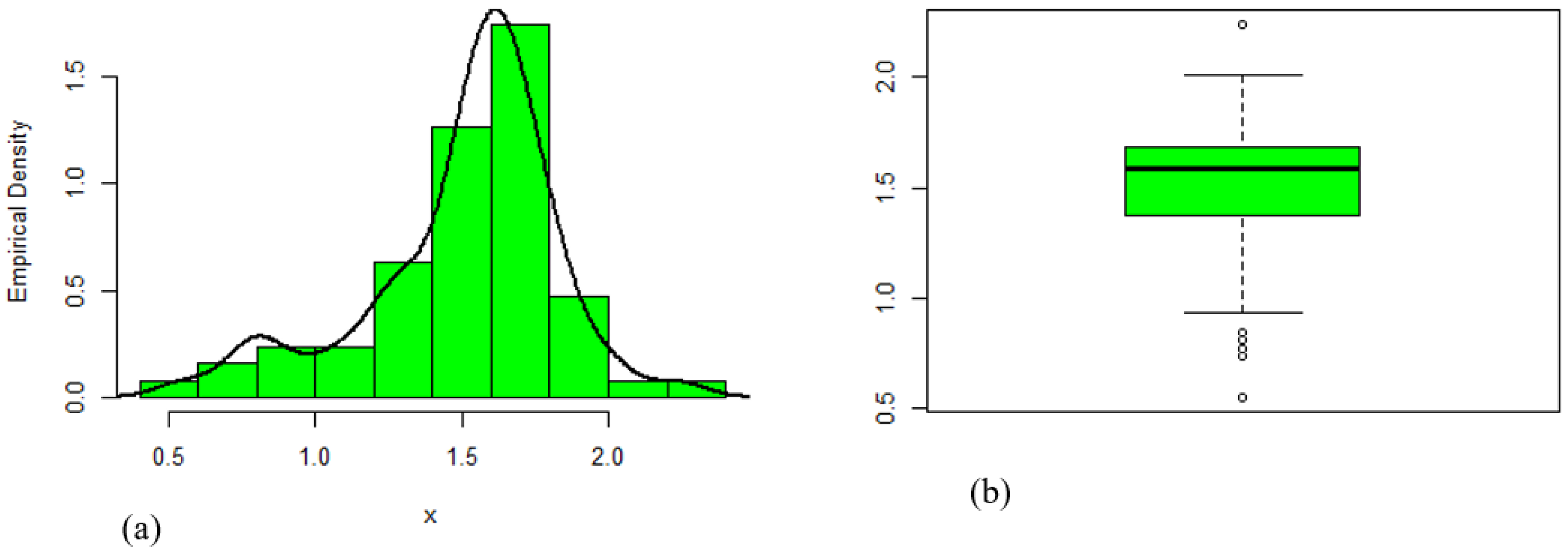
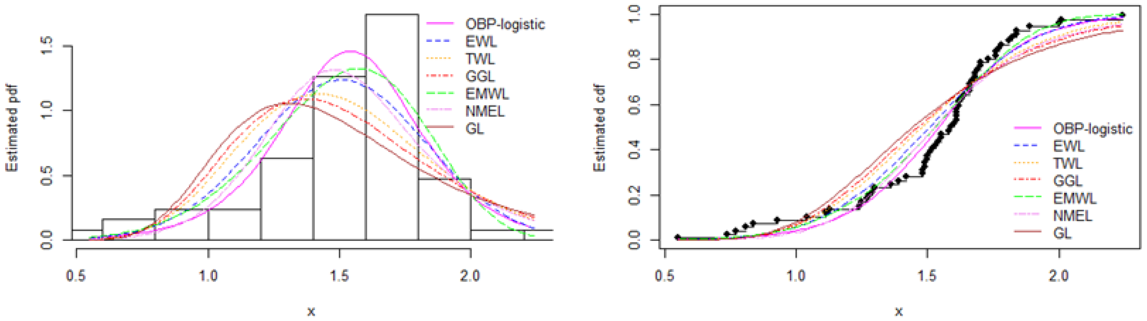
8.1. Data Set 1: Glass Fiber Data

These data were collected from the UK National Physical Laboratory and were utilized to illustrate the potential of the WAPIE PD as used previously by [11,23,81,82,83,84]. The observations are reported below (

Table 2. Glass fiber data.

0.55	0.74	0.77	0.81	0.84	1.24	0.93	1.04	1.11	1.13	1.30
1.25	1.27	1.28	1.29	1.48	1.36	1.39	1.42	1.48	1.51	1.49
1.49	1.50	1.50	1.55	1.52	1.53	1.54	1.55	1.61	1.58	1.59
1.60	1.61	1.63	1.61	1.61	1.62	1.62	1.67	1.64	1.66	1.66
1.66	1.70	1.68	1.69	1.70	1.78	1.73	1.76	1.76	1.77	1.89
1.81	1.82	1.84	1.84	2.00	2.01	2.24

).

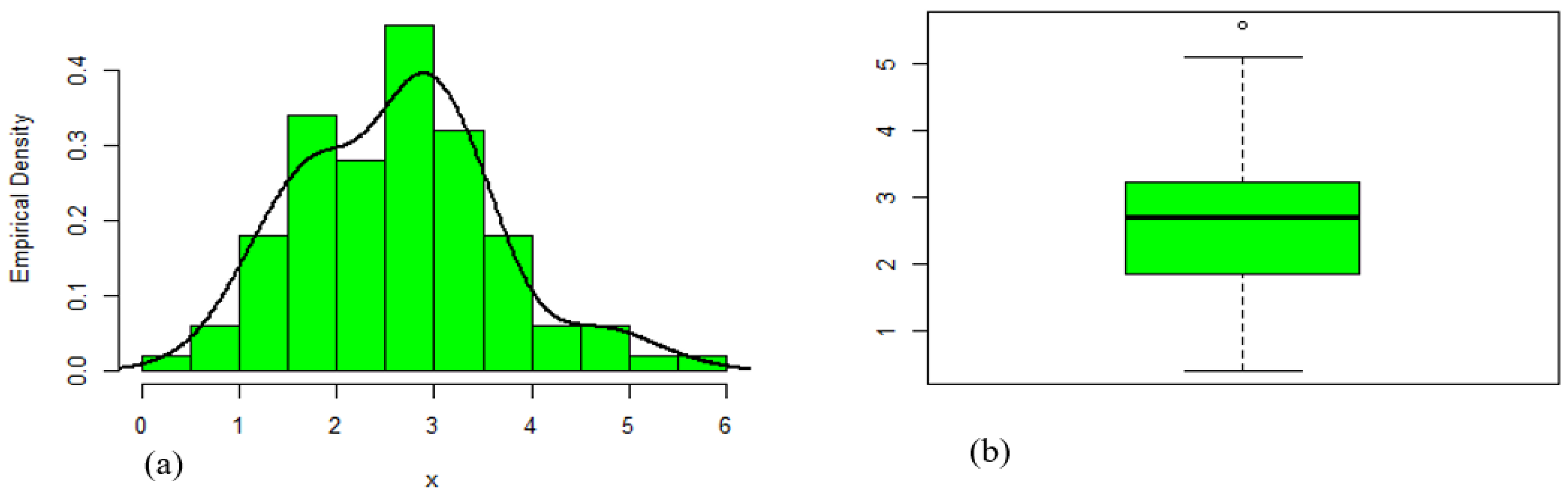
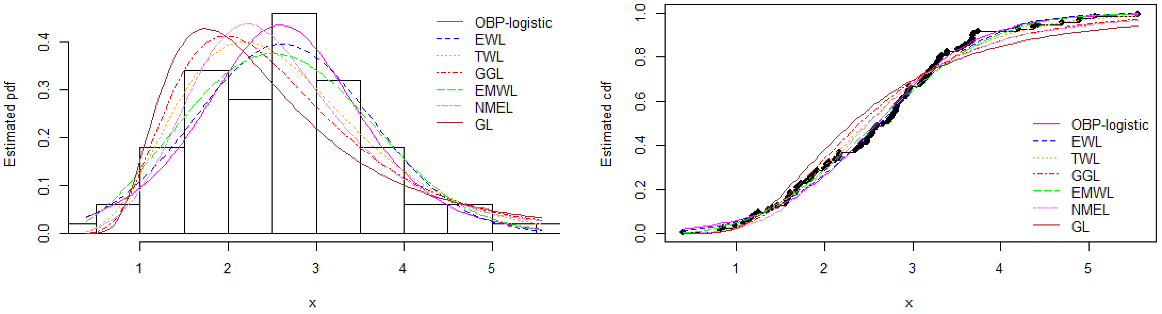
8.2. Data Set 2: Carbon Fiber Data

As used by [37], the 100 collected samples are reported below (

Table 3. Carbon fiber data.

3.70	2.74	2.73	2.50	3.60	3.11	3.27	2.87	1.47	3.11
2.41	3.19	3.22	1.69	3.28	3.09	1.87	3.15	4.90	3.75
2.95	2.97	3.39	2.96	2.53	2.67	2.93	3.22	3.39	2.81
3.33	2.55	3.31	3.31	2.85	2.56	3.56	3.15	2.35	2.55
2.38	2.81	2.77	2.17	2.83	1.92	1.41	3.68	2.97	1.36
2.76	4.91	3.68	1.84	1.59	3.19	1.57	0.81	5.56	1.73
2.00	1.22	1.12	1.71	2.17	1.17	5.08	2.48	1.18	3.51
1.69	1.25	4.38	1.84	0.39	3.68	2.48	0.85	1.61	2.79
2.03	1.80	1.57	1.08	2.03	1.61	2.12	1.89	2.88	2.82
2.05	2.43	4.20	2.59	0.98	1.59	2.17	4.70	4.42	3.65

).

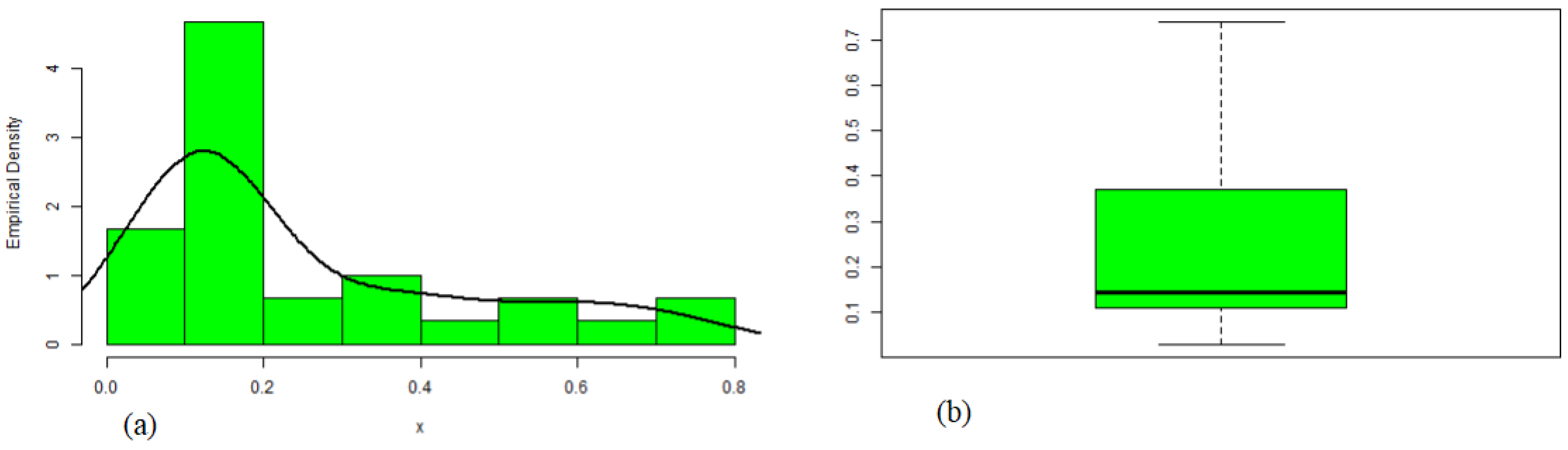
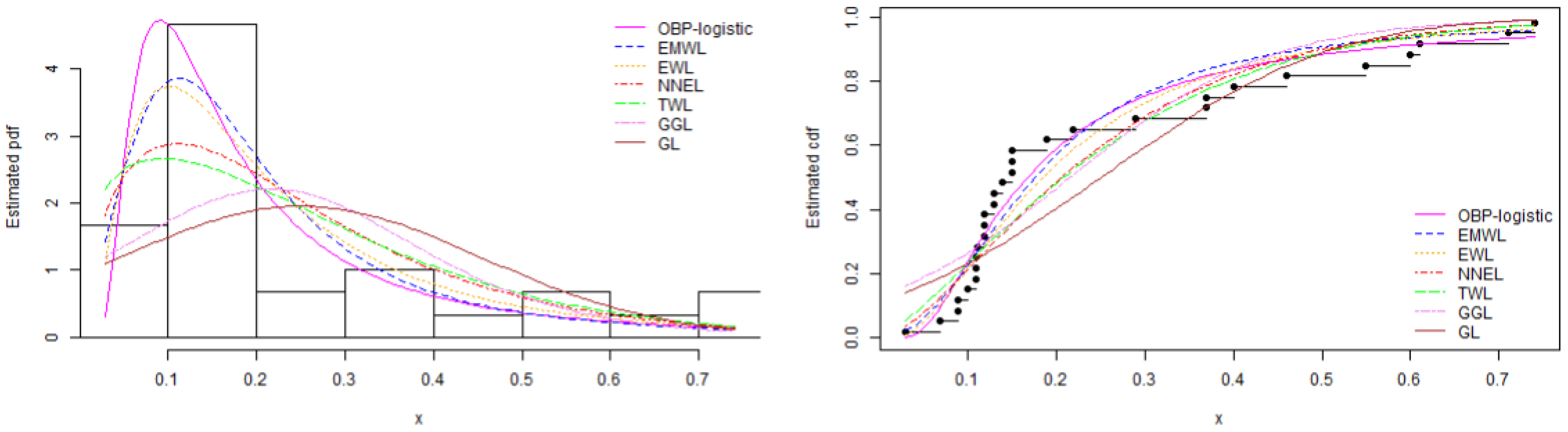
8.3. Data Set 3: Magnesium Concentration Data

Ensuring clean water and sanitation is crucial for promoting the good health and well-being of an increasing population. These data were studied by [85] to assess the magnesium concentrations for the groundwater quality. The data set is given below (

Table 4. Magnesium concentration data.

0.74	0.15	0.37	0.07	0.12	0.03	0.29	0.11	0.11	0.37
0.12	0.09	0.61	0.13	0.15	0.19	0.11	0.15	0.10	0.60
0.09	0.71	0.12	0.40	0.55	0.11	0.14	0.13	0.46	0.22

).

Table 5. Statistical summary for the GF, CF, and MC data sets.

Data	Min.	Q1	Median	Mean	Q3	Max.	Variance	Skewness	Kurtosis
1	0.550	1.375	1.590	1.507	1.685	2.240	0.105	−0.879	0.800
2	0.390	1.840	2.700	2.621	3.220	5.560	1.028	0.363	0.043
3	0.030	0.110	0.145	0.251	0.370	0.740	0.043	1.077	−0.269

depicts the statistical summary for the GF, CF and MC data sets alongside their empirical density and box plots, as shown in Figure 3a,b, Figure 4a,b and Figure 5a,b. The figures indicate that the distribution of the GF data set was skewed to the left, while the CF and MC data sets were skewed to the right, respectively. Therefore, the OBP-logistic distribution could provide a suitable fit for these types of data sets.

The MLEs with corresponding standard errors (SEs) for the OBP-logistic and competing models (GGL, NMEL, GL, EMWL, EWL, and TWL) fitted to the GF, CF and MC data are presented in

Table 6. MLEs with corresponding standard errors (in parentheses) of competitive models for GF data.

Model	$\widehat{\mathbf{a}}$	$\widehat{\mathbf{b}}$	$\widehat{\mathbf{\mu }}$	$\widehat{\mathbf{s}}$	$\widehat{\mathbf{\lambda }}$	$\widehat{\mathbf{t}}$
OBP-logistic	0.6345 (0.1279)	0.7346 (0.1671)	1.5415 (0.0368)	0.1708 (0.0184)	_	_
GGL	0.3811 (0.0325)	0.2578 (0.0229)	_	0.2854 (0.0425)	0.1764 (0.0124)	_
NMEL	_	7.9262 (0.8735)	1.5262 (0.0408)	0.5286 (0.0437)	0.8543 (0.0267)	_
GL	13.1164 (2.3079)	18.4734 (3.3134)	_	4.8783 (0.8954)	2.6508 (0.7354)	_
EMWL	5.7806 (0.5761)	1.62813 (0.0371)	_	1.2532 (0.0192)	0.3518 (0.0113)	_
EWL	0.2791 (0.0274)	0.3215 (0.0286)	_	0.4176 (0.0210)	1.5068 (0.0405)	_
TWL	17.4410 (3.0783)	_	_	8.3092 (1.7391)	11.5746 (2.0725)	2.6301 (0.6390)

,

Table 7. MLEs with corresponding standard errors (in parentheses) of competitive models for CF data.

Model	$\widehat{\mathbf{a}}$	$\widehat{\mathbf{b}}$	$\widehat{\mathbf{\mu }}$	$\widehat{\mathbf{s}}$	$\widehat{\mathbf{\lambda }}$	$\widehat{\mathbf{t}}$
OBP-logistic	0.5876 (0.1134)	0.6753 (0.3452)	2.5975 (0.1001)	0.5732 (0.0475)	_	_
GGL	0.8774 (0.0444)	0.4439 (0.0314)	_	0.7354 (0.0649)	0.2763 (0.0873)	_
NMEL	_	4.1184 (0.3441)	2.4985 (0.1053)	1.8534 (0.0342)	0.5285 (0.0263)	_
GL	4.4477 (0.6068)	9.5189 (1.3750)	_	1.4567 (0.0326)	3.0653 (0.4375)	_
EMWL	2.7929 (0.2141)	2.9438 (0.1110)	_	0.7393 (0.0741)	0.2481 (0.0173)	_
EWL	1.4502 (0.0807)	2.6214 (0.1008)	_	1.3092 (0.0981)	1.0088 (0.0713)	_
TWL	5.9529 (0.8194)	_	_	3.7407 (0.3681)	2.2711 (0.3264)	0.7622 (0.0137)

and

Table 8. MLEs with corresponding standard errors (in parentheses) of competitive models for MC data.

Model	$\widehat{\mathbf{a}}$	$\widehat{\mathbf{b}}$	$\widehat{\mathbf{\mu }}$	$\widehat{\mathbf{s}}$	$\widehat{\mathbf{\lambda }}$	$\widehat{\mathbf{t}}$
OBP-logistic	1.3290 (0.1827)	0.2756 (0.0401)	1.7834 (0.0854)	0.1964 (0.0543)	_	_
GGL	0.2162 (0.0360)	0.1129 (0.017)	_	1.9743 (0.6342)	0.3714 (0.0302)	_
NMEL	3.5783 (1.0428)	1.7937 (0.4270)	7.1363 (1.957)	1.6453 (0.4943)	_	_
GL	0.2513 (0.037)	0.2040 (0.0263)	_	1.5462 (0.3648)	0.6328 (0.0843)	_
EMWL	2.2019 (0.3317)	0.1765 (0.0258)	_	1.7845 (0.1534)	0.5281 (0.0848)	_
EWL	1.6847 (0.1418)	0.7768 (0.1002)	_	2.4271 (0.5832)	1.3977 (0.1143)	_
TWL	1.3290 (0.1827)	_	_	0.2756 (0.0402)	3.8262 (1.9436)	1.6749 (0.5483)

, respectively. The statistical metrics, $-\widehat{\mathcal{l}}$, AIC, BIC, CM, and AD, are shown in

Table 9. Statistical metrics for GF data.

Model	$-\widehat{\mathcal{l}}$	AIC	BIC	KS	CM	AD	p-Value (KS)
OBP-logistic	15.0212	34.0419	38.3281	0.12529	0.17247	1.21460	0.83122
GGL	28.0055	60.0098	64.2961	0.23127	0.69182	3.77362	0.29976
NMEL	23.7893	51.5799	56.8662	0.22365	0.50593	2.37584	0.36177
GL	33.1273	70.2546	74.5409	0.24835	0.86135	4.63834	0.20137
EMWL	17.2067	39.4136	44.6999	0.20221	0.27504	1.28061	0.71306
EWL	16.9118	36.8236	40.1099	0.13127	0.24538	1.24988	0.76951
TWL	22.9515	49.9030	53.1893	0.21636	0.36580	3.08700	0.53102

,

Table 10. Statistical metrics for CF data.

Model	$-\widehat{\mathcal{l}}$	AIC	BIC	KS	CM	AD	p-Value (KS)
OBP-logistic	141.310	287.621	291.831	0.05753	0.06165	0.42792	0.90347
GGL	148.419	300.839	306.050	0.11773	0.27528	1.46502	0.60725
NMEL	143.779	293.559	301.769	0.09025	0.15750	0.73771	0.68425
GL	158.737	321.474	326.684	0.14673	0.51933	2.84714	0.54792
EMWL	141.529	288.058	292.268	0.06049	0.06331	0.43769	0.73061
EWL	143.270	290.540	294.751	0.06306	0.06806	0.46805	0.72370
TWL	146.233	296.467	302.677	0.09339	0.16002	1.07584	0.62563

and

Table 11. Statistical metrics for MC data.

Model	$\widehat{\mathcal{l}}$	AIC	BIC	KS	CM	AD	p-Value (KS)
OBP-logistic	14.1082	−26.2164	−23.4140	0.15834	0.13164	0.83862	0.88436
GGL	18.7392	−6.38254	−3.5801	0.24248	0.38390	2.39556	0.25342
NMEL	14.8236	−24.1073	−21.2049	0.24678	0.29601	1.52516	0.46418
GL	22.7643	−6.21814	−3.4157	0.29029	0.49237	2.65561	0.20345
EMWL	14.8047	−25.6695	−22.8671	0.18878	0.18968	1.10471	0.75396
EWL	15.5494	−24.0988	−22.9964	0.20769	0.20388	1.09361	0.69807
TWL	16.2846	−22.5692	−19.7668	0.24051	0.28781	1.50597	0.37649

, respectively. From these tables, the OBP-logistic model revealed the lowest values of $-\widehat{\mathcal{l}}$, AIC, BIC, CM, and AD statistics in comparison to other competitive models. Thus, the OBP-logistic model can be selected as the best-fitting model for the GF and CF data sets. Moreover, plots in Figure 6, Figure 7 and Figure 8 also confirm these findings.

9. Discussion

This work introduces the family of probability distributions using the approach proposed by [55] to generate a compound distribution with more flexibility. The proposed family was used to develop the extended version of the logistic distribution as a sub-model. The pdf of the extended odd beta prime-logistic distribution and hazard function provided decreasing and increasing shapes, which is suitable for modeling many practical data sets from biological, environmental, finance, and engineering fields. The performance of the parameter estimates of the developed model were validated using the Monte Carlo simulation. The results from the simulation study revealed that the estimates tend to be closer to their actual values when $\mathrm{n}$ increases. In addition, the values of the error measures of the parameter estimates decrease when $\mathrm{n}$ increases. These findings provide evidence that the MLE approach generates consistent and reliable estimates for the proposed distribution across a wide range of parameter value selections. The numerical results obtained by using the statistical measure of accuracy, such as the $-\widehat{\mathcal{l}}$, AIC, BIC, CM, AD, and KS statistics, in comparison to other competitive models and the results are presented in Table 9, Table 10 and Table 11. According to these tables, the OBP-logistic model revealed the smallest values of $-\widehat{\mathcal{l}}$, AIC, BIC, CM, AD, and KS statistics in comparison to other competitive models. The numerical results presented in Table 9, Table 10 and Table 11 demonstrate that the OBP-logistic model consistently outperforms the other competitive models, as indicated by the smallest values of the aforementioned statistical measures. This suggests that the developed model exhibits superior flexibility and accuracy in fitting the data compared to the existing distributions. It is worth noting that all mathematical formulations and computations were implemented using the R Studio software. This ensures that the results are reproducible and reliable, contributing to the robustness of the study.

Overall, this paper introduces the OBP-G family of distributions and focuses on the OBP-logistic distribution as a notable member of this family. We provide a comprehensive analysis of its statistical properties, applicability to real data sets, and performance compared to other established distributions. The findings suggest that the OBP-logistic distribution offers significant advantages and is a promising choice for modeling a wide range of data sets.

10. Conclusions

In this paper, we present a novel family of probability distributions called the odd beta prime generalized (OBP-G) family of distributions. We discuss the cumulative distribution function (CDF), probability density function (PDF), and mixture representations of this new family. Additionally, we propose a new distribution within this family, namely the OBP-logistic distribution. The OBP-logistic distribution is developed based on the OBP-G family and offers a flexible modeling approach for various types of data sets. The probability density and hazard rate functions of the OBP-logistic distribution demonstrate its capability to handle skewed, symmetric, monotonically decreasing, and decreasing lifetime data. To assess the statistical properties of the OBP-logistic distribution, we define and derive several desirable features. Furthermore, we apply the maximum likelihood estimation (MLE) method to obtain estimators for the distribution’s parameters. To demonstrate the practicality of the OBP-logistic distribution, we compare it with well-established extended logistic distributions using three real data sets. We employ various statistical accuracy measures to assess the performance of the proposed distribution. The results reveal that the OBP-logistic distribution outperforms the competing distributions in terms of statistical accuracy.

For future research, this study can be extended by employing alternative methods for parameter estimation, such as the Bayesian approach, which can be preferred to make inferences regarding the unknown parameters of the model. It is also possible to assess the applicability of the new model using other data sets from various fields, such as medical sciences and finance. The study can also be improved by obtaining the properties of the OBP-G FPDs that are not covered in this paper.

References

1. Eliwa, M.S.; Altun, E.; Alhussain, Z.A.; Ahmed, E.A.; Salah, M.M.; Ahmed, H.H.; El-Morshedy, M. A new one-parameter lifetime distribution and its regression model with applications. PLoS ONE 2021, 16, e0246969. [Google Scholar] [CrossRef] [PubMed]
2. Nasiru, S. Extended Odd Fréchet-G Family of Distributions. J. Probab. Stat. 2018, 2018, 2931326. [Google Scholar] [CrossRef]
3. El-Morshedy, M.; Alshammari, F.S.; Hamed, Y.S.; Eliwa, M.S.; Yousof, H.M. A New Family of Continuous Probability Distributions. Entropy 2021, 23, 194. [Google Scholar] [CrossRef]
4. Yousof, H.M.; Altun, E.; Ramires, T.G.; Alizadeh, M.; Rasekhi, M. A new family of distributions with properties, regression models and applications. J. Stat. Manag. Syst. 2018, 21, 163–188. [Google Scholar] [CrossRef]
5. Eugene, N.; Lee, C.; Famoye, F. Beta-normal distribution and its applications. Commun. Stat.-Theory Methods 2002, 31, 497–512. [Google Scholar] [CrossRef]
6. Zografos, K.; Balakrishnan, N. On families of beta-and generalized gamma-generated distributions and associated inference. Stat. Methodol. 2009, 6, 344–362. [Google Scholar] [CrossRef]
7. Nadarajah, S.; Cordeiro, G.M.; Ortega, E.M. General results for the Kumaraswamy-G distribution. J. Stat. Comput. Simul. 2012, 82, 951–979. [Google Scholar] [CrossRef]
8. Cordeiro, G.M.; Ortega, E.M.; da Cunha, D.C. The exponentiated generalized class of distributions. J. Data Sci. 2013, 11, 1–27. [Google Scholar] [CrossRef]
9. Lee, C.; Famoye, F.; Alzaatreh, A.Y. Methods for generating families of univariate continuous distributions in the recent decades. Wiley Interdiscip. Rev. Comput. Stat. 2013, 5, 219–238. [Google Scholar] [CrossRef]
10. Cordeiro, G.M.; Alizadeh, M.; Ortega, E.M. The exponentiated half-logistic family of distributions: Properties and applications. J. Probab. Stat. 2014, 2014. [Google Scholar] [CrossRef]
11. Bourguignon, M.; Silva, R.B.; Cordeiro, G.M. The Weibull-G family of probability distributions. J. Data Sci. 2014, 12, 53–68. [Google Scholar] [CrossRef]
12. Tahir, M.H.; Cordeiro, G.M.; Alizadeh, M.; Mansoor, M.; Zubair, M.; Hamedani, G.G. The odd generalized exponential family of distributions with applications. J. Stat. Distrib. Appl. 2015, 2, 1–28. [Google Scholar] [CrossRef] [Green Version]
13. Amal, S.H.; Elgarhy, M. A New Family of Exponentiated Weibull-Generated Distributions. Int. J. Math. Its Appl. 2016, 4, 135–148. [Google Scholar]
14. Afify, A.Z.; Altun, E.; Alizadeh, M.; Ozel, G.; Hamedani, G. The odd exponentiated half-logistic-G family: Properties, characterizations and applications. Chil. J. Stat. 2017, 8, 65–91. [Google Scholar]
15. Gomes-Silva, F.S.; Percontini, A.; de Brito, E.; Ramos, M.W.; Venâncio, R.; Cordeiro, G.M. The odd Lindley-G family of distributions. Austrian J. Stat. 2017, 46, 65–87. [Google Scholar] [CrossRef] [Green Version]
16. Reyad, H.; Alizadeh, M.; Jamal, F.; Othman, S. The Topp Leone odd Lindley-G family of distributions: Properties and applications. J. Stat. Manag. Syst. 2018, 21, 1273–1297. [Google Scholar] [CrossRef]
17. ul Haq, M.A.; Elgarhy, M. The odd Frèchet-G family of probability distributions. J. Stat. Appl. Probab. 2018, 7, 189–203. [Google Scholar] [CrossRef]
18. Alizadeh, M.; Rasekhi, M.; Yousof, H.M.; Hamedani, G. The transmuted Weibull-G family of distributions. Hacet. J. Math. Stat. 2018, 47, 1671–1689. [Google Scholar] [CrossRef]
19. Oluyede, B. The gamma-Weibull-G Family of distributions with applications. Austrian J. Stat. 2018, 47, 45–76. [Google Scholar] [CrossRef] [Green Version]
20. Hassan, A.S.; Nassr, S.G. Power Lindley-G family of distributions. Ann. Data Sci. 2019, 6, 189–210. [Google Scholar] [CrossRef]
21. Ahmad, Z.; Elgarhy, M.; Hamedani, G.; Butt, N.S. Odd generalized NH generated family of distributions with application to exponential model. Pak. J. Stat. Oper. Res. 2020, 16, 53–71. [Google Scholar] [CrossRef]
22. Jamal, F.; Reyad, H.; Chesneau, C.; Nasir, M.A.; Othman, S. The Marshall-Olkin odd Lindley-G family of distributions: Theory and applications. Punjab Univ. J. Math. 2020, 51, 7. [Google Scholar]
23. Ishaq, A.I.; Abiodun, A.A. The Maxwell–Weibull distribution in modeling lifetime datasets. Ann. Data Sci. 2020, 7, 639–662. [Google Scholar] [CrossRef]
24. Al-Moisheer, A.S.; Elbatal, I.; Almutiry, W.; Elgarhy, M. Odd Inverse Power Generalized Weibull Generated Family of Distributions: Properties and Applications. Math. Probl. Eng. 2021, 2021, 5082192. [Google Scholar] [CrossRef]
25. Barranco-Chamorro, I.; Iriarte, Y.A.; Gómez, Y.M.; Astorga, J.M.; Gómez, H.W. A Generalized Rayleigh Family of Distributions Based on the Modified Slash Model. Symmetry 2021, 13, 1226. [Google Scholar] [CrossRef]
26. Jamal, F.; Handique, L.; Ahmed, A.H.N.; Khan, S.; Shafiq, S.; Marzouk, W. The Generalized Odd Linear Exponential Family of Distributions with Applications to Reliability Theory. Math. Comput. Appl. 2022, 27, 55. [Google Scholar] [CrossRef]
27. Hussain, S.; Sajid Rashid, M.; Ul Hassan, M.; Ahmed, R. The Generalized Exponential Extended Exponentiated Family of Distributions: Theory, Properties, and Applications. Mathematics 2022, 10, 3419. [Google Scholar] [CrossRef]
28. Hussain, S.; Rashid, M.S.; Ul Hassan, M.; Ahmed, R. The Generalized Alpha Exponent Power Family of Distributions: Properties and Applications. Mathematics 2022, 10, 1421. [Google Scholar] [CrossRef]
29. Bourguignon, M.; Santos-Neto, M.; de Castro, M. A new regression model for positive random variables with skewed and long tail. Metron 2021, 79, 33–55. [Google Scholar] [CrossRef]
30. Kalbfleisch, J.D.; Prentice, R.L. The Statistical Analysis of Failure Time Data; John Wiley & Sons: Hoboken, NJ, USA, 2011. [Google Scholar]
31. Venter, G. Transformed beta and gamma distributions and aggregate losses. In Proceedings of Casualty Actuarial Society; Casualty Actuarial Society: Arlington, VA, USA, 1983; Volume 70, pp. 289–308. [Google Scholar]
32. Vartia, P.; Vartia, Y.O. Description of the Income Distribution by the Scaled F Distribution Model; Elinkeinoelämän Tutkimuslaitos: Helsinki, Finland, 1981. [Google Scholar]
33. McDonald, J.B.; Ransom, M.R. Functional forms, estimation techniques and the distribution of income. Econom. J. Econom. Soc. 1979, 47, 1513–1525. [Google Scholar] [CrossRef]
34. McDonald, J.B. Model selection: Some generalized distributions. Commun. Stat.-Theory Methods 1987, 16, 1049–1074. [Google Scholar] [CrossRef]
35. McDonald, J.B.; Butler, R.J. Regression models for positive random variables. J. Econom. 1990, 43, 227–251. [Google Scholar] [CrossRef]
36. Tulupyev, A.; Suvorova, A.; Sousa, J.; Zelterman, D. Beta prime regression with application to risky behavior frequency screening. Stat. Med. 2013, 32, 4044–4056. [Google Scholar] [CrossRef] [PubMed]
37. Ferreira, J.; Soares, C.G. Modelling the long-term distribution of significant wave height with the Beta and Gamma models. Ocean. Eng. 1999, 26, 713–725. [Google Scholar] [CrossRef]
38. Dubey, S.D. Compound gamma, beta and F distributions. Metrika 1970, 16, 27–31. [Google Scholar] [CrossRef]
39. Joshi, R.K.; Kumar, V. The Logistic Gompertz Distribution with Properties and Applications. Bull. Math. Stat. Res. 2020, 8, 81–94. [Google Scholar]
40. Brown, R.Z. Social behavior, reproduction, and population changes in the house mouse (Mus musculus L.). Ecol. Monogr. 1953, 23, 218–240. [Google Scholar] [CrossRef]
41. Schultz, H. The standard error of a forecast from a curve. J. Am. Stat. Assoc. 1930, 25, 139–185. [Google Scholar] [CrossRef]
42. Oliver, F. Methods of estimating the logistic growth function. J. R. Stat. Soc. Ser. C (Appl. Stat.) 1964, 13, 57–66. [Google Scholar] [CrossRef]
43. Ravikumar, K. Negative Binomial Logistic Distribution. Turk. J. Comput. Math. Educ. (TURCOMAT) 2021, 12, 5963–5976. [Google Scholar]
44. Johnson, N.L.; Kotz, S.; Balakrishnan, N. Continuous Univariate Distributions, Volume 2; John Wiley & Sons: Hoboken, NJ, USA, 1995. [Google Scholar]
45. Alzaatreh, A.; Ghosh, I.; Said, H. On the gamma-logistic distribution. J. Mod. Appl. Stat. Methods 2014, 13, 5. [Google Scholar] [CrossRef] [Green Version]
46. Morais, A.L.; Cordeiro, G.M.; Cysneiros, A.H. The beta generalized logistic distribution. Braz. J. Probab. Stat. 2013, 27, 185–200. [Google Scholar] [CrossRef]
47. Prentice, R.L. A generalization of the probit and logit methods for dose response curves. Biometrics 1976, 32, 761–768. [Google Scholar] [CrossRef] [PubMed]
48. Stukel, T.A. Generalized logistic models. J. Am. Stat. Assoc. 1988, 83, 426–431. [Google Scholar] [CrossRef]
49. Balakrishnan, N.; Leung, M. Order statistics from the type I generalized logistic distribution. Commun. Stat.-Simul. Comput. 1988, 17, 25–50. [Google Scholar] [CrossRef]
50. Wahed, A.; Ali, M.M. The skew-logistic distribution. J. Statist. Res 2001, 35, 71–80. [Google Scholar]
51. Nadarajah, S. The skew logistic distribution. AStA Adv. Stat. Anal. 2009, 93, 187–203. [Google Scholar] [CrossRef]
52. Gupta, R.D.; Kundu, D. Generalized logistic distributions. J. Appl. Stat. Sci. 2010, 18, 51. [Google Scholar]
53. Azzalini, A. A class of distributions which includes the normal ones. Scand. J. Stat. 1985, 12, 171–178. [Google Scholar]
54. Aljarrah, M.A.; Famoye, F.; Lee, C. Generalized logistic distribution and its regression model. J. Stat. Distrib. Appl. 2020, 7, 1–21. [Google Scholar] [CrossRef]
55. Alzaatreh, A.; Lee, C.; Famoye, F. A new method for generating families of continuous distributions. Metron 2013, 71, 63–79. [Google Scholar] [CrossRef] [Green Version]
56. Aljarrah, M.A.; Lee, C.; Famoye, F. On generating TX family of distributions using quantile functions. J. Stat. Distrib. Appl. 2014, 1, 1–17. [Google Scholar] [CrossRef]
57. Ghosh, I.; Alzaatreh, A. A new class of generalized logistic distribution. Commun. Stat.-Theory Methods 2018, 47, 2043–2055. [Google Scholar] [CrossRef]
58. Suleiman, A.; Othman, M.; Ishaq, A.; Daud, H.; Indawati, R.; Abdullah, M.L.; Husin, A. The Odd Beta Prime-G Family of Probability Distributions: Properties and Applications. In Proceedings of the 1st International Online Conference on Mathematics and Applications, Online, 1–15 May 2023; MDPI: Basel, Switzerland, 2023. [Google Scholar] [CrossRef]
59. Alsadat, N.; Ahmad, A.; Jallal, M.; Gemeay, A.M.; Meraou, M.A.; Hussam, E.; Elmetwally, E.M.; Hossain, M.M. The novel Kumaraswamy power Frechet distribution with data analysis related to diverse scientific areas. Alex. Eng. J. 2023, 70, 651–664. [Google Scholar] [CrossRef]
60. Alghamdi, S.M.; Shrahili, M.; Hassan, A.S.; Mohamed, R.E.; Elbatal, I.; Elgarhy, M. Analysis of Milk Production and Failure Data: Using Unit Exponentiated Half Logistic Power Series Class of Distributions. Symmetry 2023, 15, 714. [Google Scholar] [CrossRef]
61. Muhammad, M.; Bantan, R.A.R.; Liu, L.; Chesneau, C.; Tahir, M.H.; Jamal, F.; Elgarhy, M. A New Extended Cosine—G Distributions for Lifetime Studies. Mathematics 2021, 9, 2758. [Google Scholar] [CrossRef]
62. Alyami, S.A.; Elbatal, I.; Alotaibi, N.; Almetwally, E.M.; Elgarhy, M. Modeling to Factor Productivity of the United Kingdom Food Chain: Using a New Lifetime-Generated Family of Distributions. Sustainability 2022, 14, 8942. [Google Scholar] [CrossRef]
63. Alyami, S.A.; Babu, M.G.; Elbatal, I.; Alotaibi, N.; Elgarhy, M. Type II Half-Logistic Odd Fr&eacute;chet Class of Distributions: Statistical Theory and Applications. Symmetry 2022, 14, 1222. [Google Scholar]
64. Elbatal, I.; Alotaibi, N.; Almetwally, E.M.; Alyami, S.A.; Elgarhy, M. On Odd Perks-G Class of Distributions: Properties, Regression Model, Discretization, Bayesian and Non-Bayesian Estimation, and Applications. Symmetry 2022, 14, 883. [Google Scholar] [CrossRef]
65. Alotaibi, N.; Elbatal, I.; Almetwally, E.M.; Alyami, S.A.; Al-Moisheer, A.S.; Elgarhy, M. Truncated Cauchy Power Weibull-G Class of Distributions: Bayesian and Non-Bayesian Inference Modelling for COVID-19 and Carbon Fiber Data. Mathematics 2022, 10, 1565. [Google Scholar] [CrossRef]
66. Algarni, A.; Almarashi, A.M.; Elbatal, I.; Hassan, A.S.; Almetwally, E.M.; Daghistani, A.M.; Elgarhy, M. Type I Half Logistic Burr X-G Family: Properties, Bayesian, and Non-Bayesian Estimation under Censored Samples and Applications to COVID-19 Data. Math. Probl. Eng. 2021, 2021, 5461130. [Google Scholar] [CrossRef]
67. David Sam Jayakumar, G.S.; Sulthan, A.; Samuel, W. A new bivariate beta distribution of Kind-1 of Type-A. J. Stat. Manag. Syst. 2019, 22, 141–158. [Google Scholar] [CrossRef]
68. Baro-Tijerina, M.; Pina-Monarrez, M.R.; Villa-Covarrubias, B. Stress-strength Weibull analysis with different shape parameter and probabilistic safety factor. DYNA 2020, 87, 28–33. [Google Scholar] [CrossRef]
69. Gauss, M.C.; Saralees, N. Closed-form expressions for moments of a class of beta generalized distributions. Braz. J. Probab. Stat. 2011, 25, 14–33. [Google Scholar] [CrossRef]
70. Verma, A. Finite summation formulas of generalized Kampé de Fériet series. arXiv 2020, arXiv:2003.07530. [Google Scholar]
71. Rényi, A. On measures of entropy and information. In Proceedings of the Fourth Berkeley Symposium on Mathematical Statistics and Probability, Berkeley, CA, USA, 20 June–30 July 1960; University of California Press: Berkeley, CA, USA; Volume 1, pp. 547–561. [Google Scholar]
72. Khammash, G.S.; Agarwal, P.; Choi, J. Extended k-Gamma and k-Beta Functions of Matrix Arguments. Mathematics 2020, 8, 1715. Available online: https://www.mdpi.com/2227-7390/8/10/1715 (accessed on 16 March 2023). [CrossRef]
73. R Core Team. R: A Language and Environment for Statistical Computing; R Foundation for Statistical Computing: Vienna, Austria, 2022; Available online: https://cir.nii.ac.jp/crid/1574231874043578752 (accessed on 5 April 2023).
74. Kumar, C.S.; Manju, L. Gamma Generalized Logistic Distribution: Properties and Applications. J. Stat. Theory Appl. 2022, 21, 155–174. [Google Scholar] [CrossRef]
75. Ahmad, Z.; Almaspoor, Z.; Khan, F.; Alhazmi, S.E.; El-Morshedy, M.; Ababneh, O.; Al-Omari, A.I. On fitting and forecasting the log-returns of cryptocurrency exchange rates using a new logistic model and machine learning algorithms. AIMS Math. 2022, 7, 18031–18049. [Google Scholar] [CrossRef]
76. Nassar, M.M.; Radwan, S.S.; Elmasry, A.S. the Exponential Modified Weibull Logistic Distribution (EMWL). EPH-Int. J. Math. Stat. 2018, 4, 22–38. [Google Scholar] [CrossRef]
77. MURAT, U.; Gamze, Ö. Exponentiated Weibull-logistic distribution. Bilge Int. J. Sci. Technol. Res. 2020, 4, 55–62. [Google Scholar]
78. Nassar, M.; Radwan, S.; Elmasry, A. Transmuted Weibull logistic distribution. Int. J. Innov. Res. Dev. 2017, 6, 122–131. [Google Scholar] [CrossRef] [Green Version]
79. Abdullahi, U.A.; Suleiman, A.A.; Ishaq, A.I.; Usman, A.; Suleiman, A. The Maxwell–Exponential Distribution: Theory and Application to Lifetime Data. J. Stat. Model. Anal. (JOSMA) 2021, 3, 2. [Google Scholar] [CrossRef]
80. Singh, V.V.; Suleman, A.A.; Ibrahim, A.; Abdullahi, U.A.; Suleiman, S.A. Assessment of probability distributions of groundwater quality data in Gwale area, north-western Nigeria. Ann. Optim. Theory Pract. 2020, 3, 37–46. [Google Scholar]
81. Eferhonore, E.-E.; Thomas, J.; Zelibe, S.C. Theoretical analysis of the Weibull alpha power inverted exponential distribution: Properties and applications. Gazi Univ. J. Sci. 2020, 33, 265–277. [Google Scholar]
82. Ceren, Ü.; Cakmakyapan, S.; Gamze, Ö. Alpha power inverted exponential distribution: Properties and application. Gazi Univ. J. Sci. 2018, 31, 954–965. [Google Scholar]
83. Merovci, F.; Khaleel, M.A.; Ibrahim, N.A.; Shitan, M. The beta Burr type X distribution properties with application. SpringerPlus 2016, 5, 697. [Google Scholar] [CrossRef] [Green Version]
84. Maxwell, O.; Oyamakin, S.O.; Th, E.J. The Gompertz Length Biased Exponential Distribution and its application to Uncensored Data. Curr. Trends Biostat. Biom. 2018, 1, 52–57. [Google Scholar] [CrossRef]
85. Suleiman, A.A.; Abdullahi, U.A.; Suleiman, A.; Yunus, R.B.; Suleiman, S.A. Assessment of Groundwater Quality Using Multivariate Statistical Techniques. In Intelligent Systems Modeling and Simulation II: Machine Learning, Neural Networks, Efficient Numerical Algorithm and Statistical Methods; Springer: Berlin/Heidelberg, Germany, 2022; pp. 567–579. [Google Scholar]
Figure 1. Plots of the pdf of the OBP-logistic distribution for different values of parameters. (a)–(c) show that the pdf of the OBP-logistic distribution can be symmetric, right-skewed or left-skewed density function.
Sustainability 15 10239 g001
Figure 2. Plots of the hazard rate of the OBP-logistic distribution. (a,b) show that the hazard rate of the OBP-logistic distribution can be monotonically decreasing or monotonically increasing hazard function.
Sustainability 15 10239 g002
Figure 3. The density and box plots for the GF data. (a) show negative skewness of extreme values for the GF data (b) show statistical behavior of extreme values for the GF data.
Sustainability 15 10239 g003
Figure 4. The density and box plots for the CF data. (a) show positive skewness of extreme values for the CF data (b) show statistical behavior of extreme values for the CF data.
Sustainability 15 10239 g004
Figure 5. The density and box plots for the MC data. (a) show positive skewness for the MC data (b) show negative kurtosis for the MC data.
Sustainability 15 10239 g005
Figure 6. Plots of empirical and fitted densities; and empirical cdfs and fitted cdfs for GF data.
Sustainability 15 10239 g006
Figure 7. Plots of empirical and fitted densities; and empirical cdfs and fitted cdfs for CF data.
Sustainability 15 10239 g007
Figure 8. Plots of empirical and fitted densities; and empirical cdfs and fitted cdfs for MC data.
Sustainability 15 10239 g008