

Comparison of Ratioing and RCNA Methods in the Detection of Flooded Areas Using Sentinel 2 Imagery (Case Study: Tulun, Russia)

 , ,
, ,  and
and
Abstract
1. Introduction
2. Materials and Methods
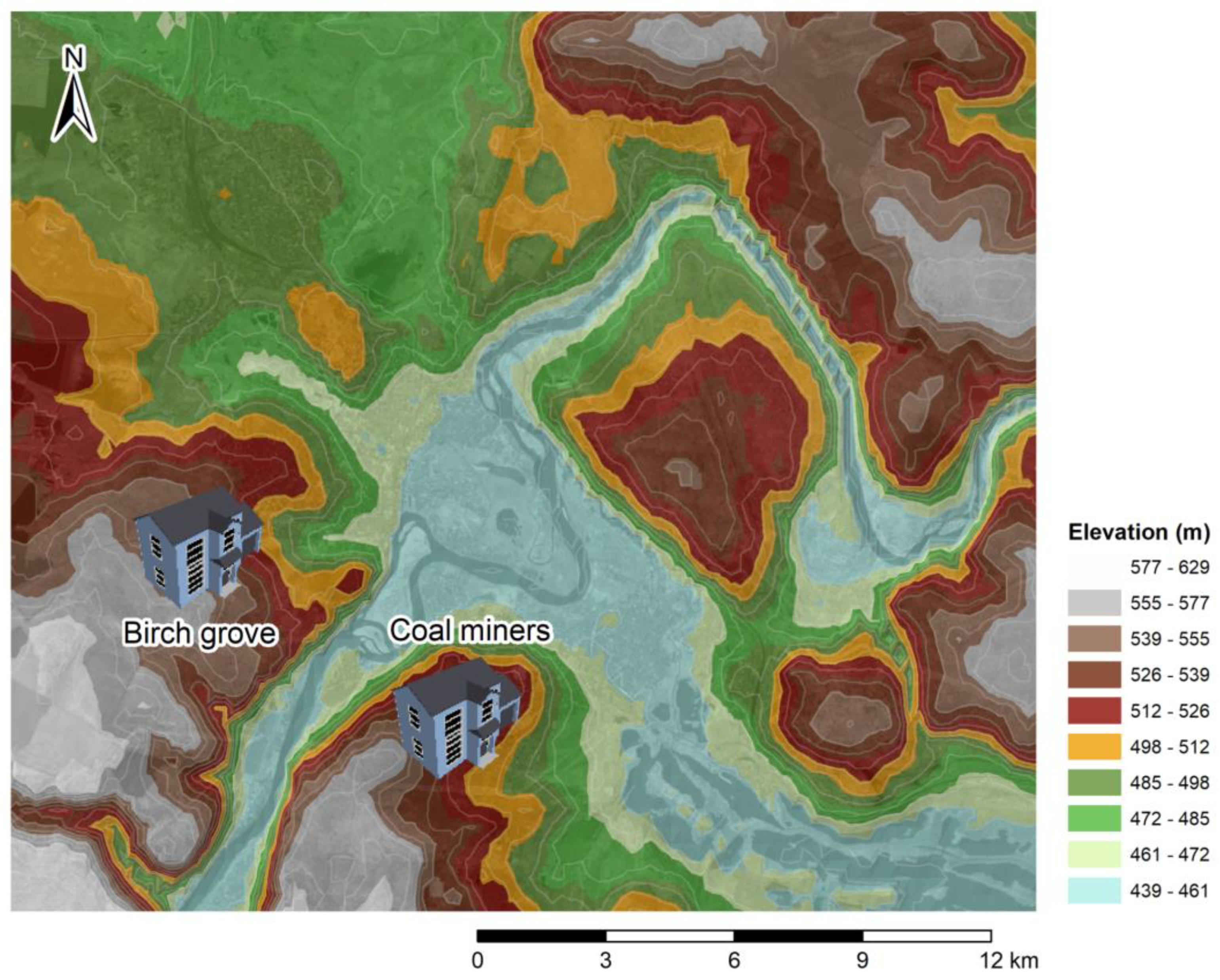
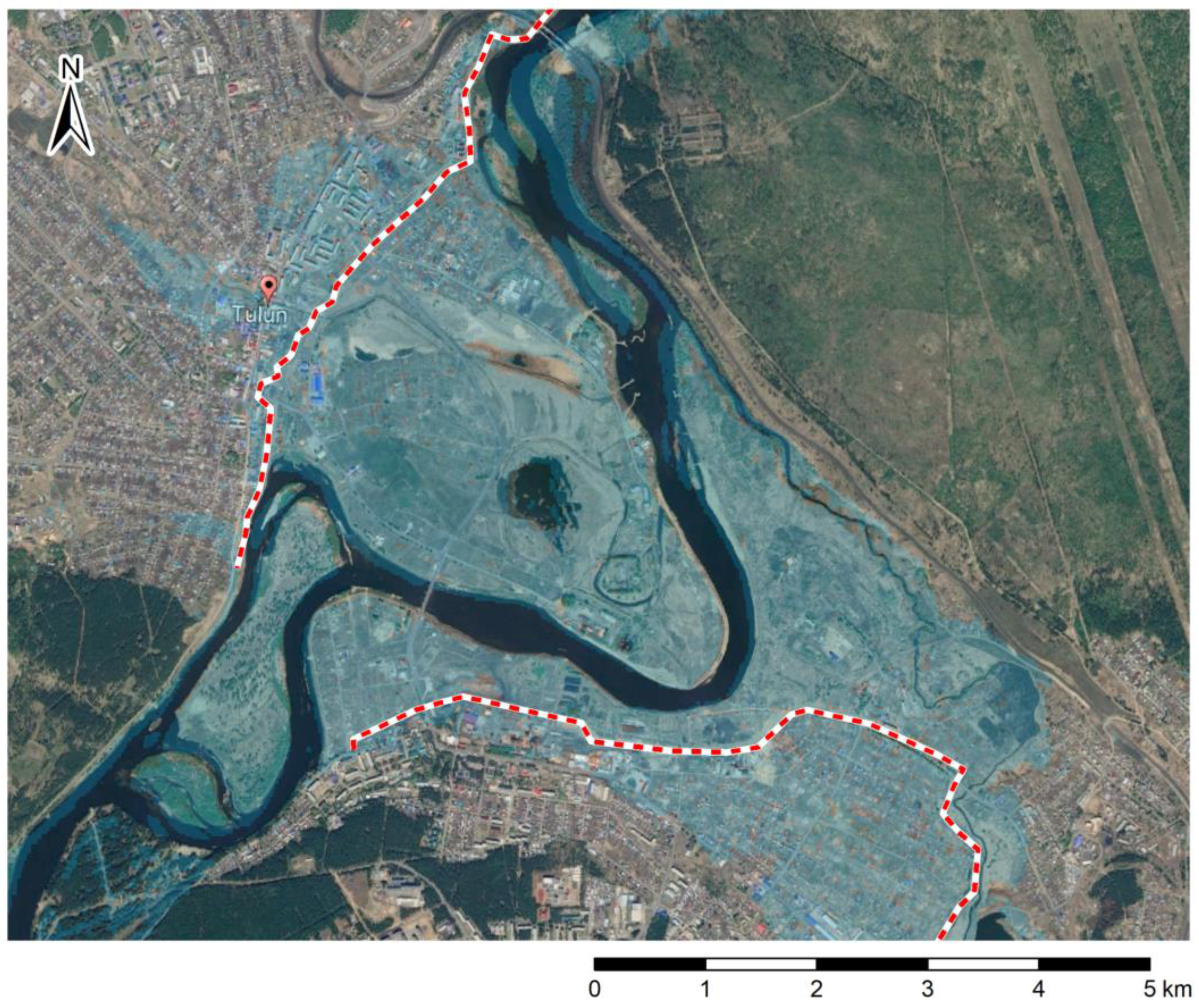
2.1. Study Area
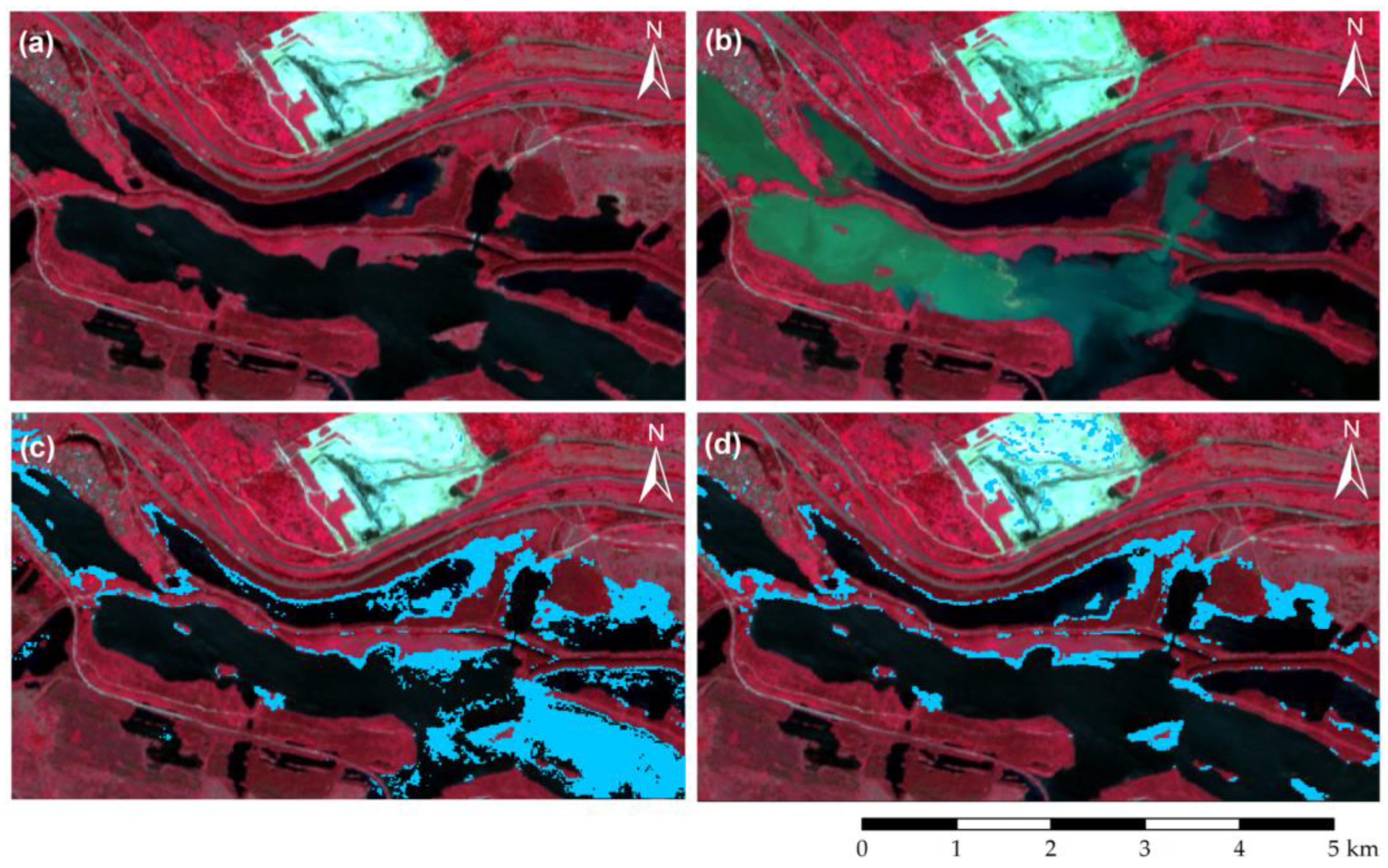
2.2. Methodology
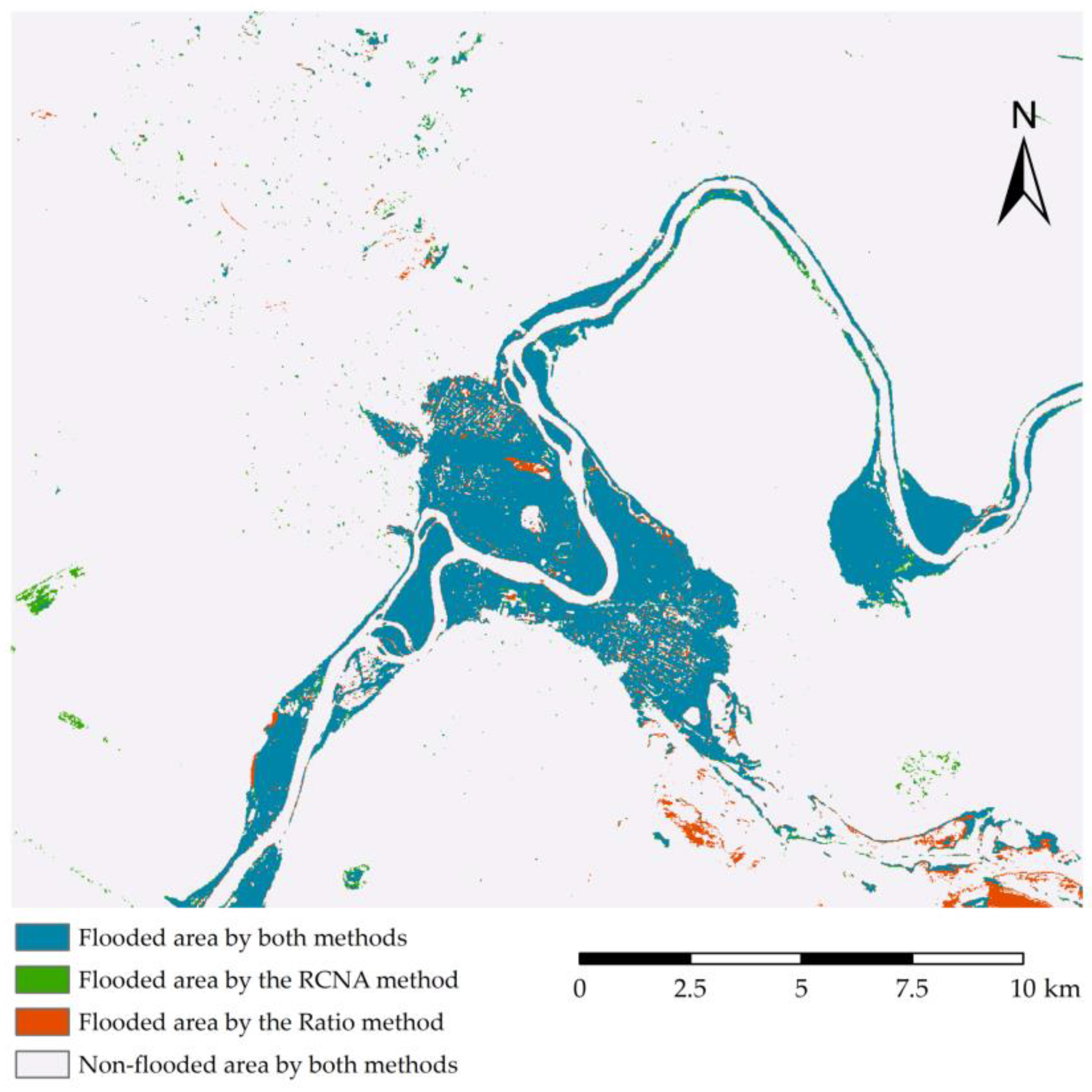
3. Results and Discussion
4. Conclusions
Author Contributions
Funding
Institutional Review Board Statement
Informed Consent Statement
Data Availability Statement
Conflicts of Interest
References
- Zandalinas, S.I.; Fritschi, F.B.; Mittler, R. Global warming, climate change, and environmental pollution: Recipe for a multifactorial stress combination disaster. Trends Plant Sci. 2021, 26, 588–599. [Google Scholar] [CrossRef] [PubMed]
- Pour, S.H.; Abd Wahab, A.K.; Shahid, S.; Asaduzzaman, M.; Dewan, A. Low impact development techniques to mitigate the impacts of climate-change-induced urban floods: Current trends, issues and challenges. Sustain. Cities Soc. 2020, 62, 102373. [Google Scholar] [CrossRef]
- Halder, B.; Bandyopadhyay, J.; Banik, P. Evaluation of the climate change impact on urban heat island based on land surface temperature and geospatial indicators. Int. J. Environ. Res. 2021, 15, 819–835. [Google Scholar] [CrossRef]
- Zhou, Q.; Leng, G.; Su, J.; Ren, Y. Comparison of urbanization and climate change impacts on urban flood volumes: Importance of urban planning and drainage adaptation. Sci. Total Environ. 2019, 658, 24–33. [Google Scholar] [CrossRef] [PubMed]
- Steensen, B.M.; Marelle, L.; Hodnebrog, Ø.; Myhre, G. Future urban heat island influence on precipitation. Clim. Dyn. 2022, 58, 3393–3403. [Google Scholar] [CrossRef]
- Hassan, B.T.; Yassine, M.; Amin, D. Comparison of urbanization, climate change, and drainage design impacts on urban flashfloods in an arid region: Case study, New Cairo, Egypt. Water 2022, 14, 2430. [Google Scholar] [CrossRef]
- Hammond, M.J.; Chen, A.S.; Djordjević, S.; Butler, D.; Mark, O. Urban flood impact assessment: A state-of-the-art review. Urban Water J. 2015, 12, 14–29. [Google Scholar] [CrossRef]
- Devi, N.N.; Sridharan, B.; Kuiry, S.N. Impact of urban sprawl on future flooding in Chennai city, India. J. Hydrol. 2019, 574, 486–496. [Google Scholar] [CrossRef]
- Chen, K.F.; Leandro, J. A conceptual time-varying flood resilience index for urban areas: Munich city. Water 2019, 11, 830. [Google Scholar] [CrossRef]
- Fletcher, T.D.; Shuster, W.; Hunt, W.F.; Ashley, R.; Butler, D.; Arthur, S.; Trowsdale, S.; Barraud, S.; Semadeni-Davies, A.; Bertrand-Krajewski, J.-L.; et al. SUDS, LID, BMPs, WSUD and more—The evolution and application of terminology surrounding urban drainage. Urban Water J. 2015, 12, 525–542. [Google Scholar] [CrossRef]
- Gimenez-Maranges, M.; Breuste, J.; Hof, A. Sustainable Drainage Systems for transitioning to sustainable urban flood management in the European Union: A review. J. Clean. Prod. 2020, 255, 120191. [Google Scholar] [CrossRef]
- Seyedashraf, O.; Bottacin-Busolin, A.; Harou, J.J. Many-Objective Optimization of Sustainable Drainage Systems in Urban Areas with Different Surface Slopes. Water Resour. Manag. 2021, 35, 2449–2464. [Google Scholar] [CrossRef]
- Green, D.; O’Donnell, E.; Johnson, M.; Slater, L.; Thorne, C.; Zheng, S.; Stirling, R.; Chan, F.K.S.; Li, L.; Boothroyd, R.J. Green infrastructure: The future of urban flood risk management? Wiley Interdiscip. Rev. Water 2021, 8, e21560. [Google Scholar] [CrossRef]
- TerraTech, J.S.C. Space Monitoring of the Flood in Tulun. Status as of July 3. 2019. Available online: https://terratech.ru/news/Tulune.pdf (accessed on 14 February 2023).
- Bolshakov, A.G. Urban planning analysis of the city of Tulun. Earth Environ. Sci. 2021, 751, 012041. [Google Scholar] [CrossRef]
- Kichigina, N.V. Flood hazard within the basins of the left tributaries of the Angara. Geogr. Nat. Resour. 2020, 41, 344–353. [Google Scholar] [CrossRef]
- Belikov, V.V.; Borisova, N.M.; Glotko, A.V. Numerical Hydrodynamic 2D-Simulation of the Inundation of Tulun Town on the Iya R. during Flood 2019. Water Resour. 2021, 48, 713–725. [Google Scholar] [CrossRef]
- D’yakonov, K.N.; Khoroshev, A.V. Landscape Planning on the Way to Integration in Regional Policy. Her. Russ. Acad. Sci. 2022, 92, 297–305. [Google Scholar] [CrossRef]
- Klemas, V. Remote sensing of floods and flood-prone areas: An overview. J. Coast. Res. 2015, 31, 1005–1013. [Google Scholar] [CrossRef]
- Sadiq, R.; Akhtar, Z.; Imran, M.; Ofli, F. Integrating remote sensing and social sensing for flood mapping. Remote Sens. Appl. Soc. Environ. 2022, 25, 100697. [Google Scholar] [CrossRef]
- Dammalage, T.L.; Jayasinghe, N.T. Land-use change and its impact on urban flooding: A case study on Colombo district flood on May 2016. Eng. Technol. Appl. Sci. Res. 2019, 9, 3887–3891. [Google Scholar] [CrossRef]
- Shahabi, H.; Shirzadi, A.; Ghaderi, K.; Omidvar, E.; Al-Ansari, N.; Clague, J.J.; Geertsema, M.; Khosravi, K.; Amini, A.; Bahrami, S.; et al. Flood detection and susceptibility mapping using sentinel-1 remote sensing data and a machine learning approach: Hybrid intelligence of bagging ensemble based on k-nearest neighbor classifier. Remote Sens. 2020, 12, 266. [Google Scholar] [CrossRef]
- Tanim, A.H.; McRae, C.B.; Tavakol-Davani, H.; Goharian, E. Flood Detection in Urban Areas Using Satellite Imagery and Machine Learning. Water 2022, 14, 1140. [Google Scholar] [CrossRef]
- Farhadi, H.; Esmaeily, A.; Najafzadeh, M. Flood monitoring by integration of Remote Sensing technique and Multi-Criteria Decision Making method. Comput. Geosci. 2022, 160, 105045. [Google Scholar] [CrossRef]
- Hashemi-Beni, L.; Gebrehiwot, A.A. Flood extent mapping: An integrated method using deep learning and region growing using UAV optical data. IEEE J. Sel. Top. Appl. Earth Obs. Remote Sens. 2021, 14, 2127–2135. [Google Scholar] [CrossRef]
- Shen, X.; Wang, D.; Mao, K.; Anagnostou, E.; Hong, Y. Inundation Extent Mapping by Synthetic Aperture Radar: A Review. Remote Sens. 2019, 11, 879. [Google Scholar] [CrossRef]
- Anusha, N.; Bharathi, B. Flood detection and flood mapping using multi-temporal synthetic aperture radar and optical data. Egypt. J. Remote Sens. Space Sci. 2020, 23, 207–219. [Google Scholar] [CrossRef]
- Tarpanelli, A.; Mondini, A.C.; Camici, S. Effectiveness of Sentinel-1 and Sentinel-2 for flood detection assessment in Eu-rope. Nat. Hazards Earth Syst. Sci. 2022, 22, 2473–2489. [Google Scholar] [CrossRef]
- Zhang, Q.; Zhang, P.; Hu, X. Unsupervised GRNN flood mapping approach combined with uncertainty analysis using bi-temporal Sentinel-2 MSI imageries. Int. J. Digital Earth 2021, 14, 1561–1581. [Google Scholar] [CrossRef]
- Akulov, N.I.; Frolov, A.O.; Mashchuk, I.M.; Akulova, V.V. Jurassic deposits of the southern part of the Irkutsk sedimentary basin. Stratigr. Geol. Correl. 2015, 23, 387–409. [Google Scholar] [CrossRef]
- Maldonado, F.D.; Santos, J.R.; Graça, P.M.L. Change detection technique based on the radiometric rotation controlled by no-change axis, applied on a semi-arid landscape. Int. J. Remote Sens. 2007, 28, 1001–1016. [Google Scholar] [CrossRef]
- Minu, S.; Shetty, A. A comparative study of image change detection algorithms in MATLAB. Aquat. Procedia 2015, 4, 1366–1373. [Google Scholar] [CrossRef]
- Hashim, M.; Watson, A.; Thomas, M. An approach for correcting in homogeneous atmospheric effects in remote sensing images. Int. J. Remote Sens. 2004, 25, 5131–5141. [Google Scholar] [CrossRef]
- Lu, D.; Mausel, P.; Batistella, M.; Moran, E. Land-cover binary change detection methods for use in the moist tropical region of the Amazon: A comparative study. Int. J. Remote Sens. 2005, 26, 101–114. [Google Scholar] [CrossRef]
- Yvonne, W.; Maier, S.W.; Dech, S.W.; Conrad, C.; Colditz, R.R. Classification of burn severity using Moderate Resolution Imaging Spectroradiometer (MODIS): A case study in the jarrah-marri forest of southwest Western Australia. J. Geophys. Res. 2007, 112, G02002. [Google Scholar] [CrossRef]
- McHugh, M.L. Interrater reliability: The kappa statistic. Biochem. Med. 2012, 22, 276–282. [Google Scholar] [CrossRef]
- Shalikovsky, A.V.; Lepikhin, A.P.; Tiunov, A.A.; Kurganovich, K.A.; Morozov, М.G. The 2019 Floods in Irkutsk Region. Вoднoе Хoзяйствo Рoссии Прoблемы Технoлoгии Управление 2019, 6, 48–65. [Google Scholar] [CrossRef]
- Sutyrina, E.N.; Antonova, T.I. SRTM data application for extrapolation of rating curves (on the example of the Iya river at the Tulun gauge). Bull. Irkutsk. State Univ. Ser. Earth Sci. 2022, 41, 140–150. [Google Scholar] [CrossRef]
- Bolshakov, A.G. Principles of reconstruction of a small depressive city on the example of Tulun. Earth Environ. Sci. 2021, 751, 012040. [Google Scholar] [CrossRef]
- RusHydro Group, JSC Institute Hydroproject. 2019. Available online: http://www.mhp.rushydro.ru/press/publications/113441.html (accessed on 1 April 2023).
- Kalugin, A. Process-based modeling of the high flow of a semi-mountain river under current and future climatic conditions: A case study of the Iya River (Eastern Siberia). Water 2021, 13, 1042. [Google Scholar] [CrossRef]


| Classes | Flooded Pixels (1) | Non-Flooded Pixels (0) | Total | Errors of Commission | User Accuracy (%) |
|---|---|---|---|---|---|
| Flooded (1) | 56 | 27 | 83 | 0.33 | 67.47 |
| Non-flooded (0) | 6 | 111 | 117 | 0.05 | 94.87 |
| Total | 62 | 138 | 200 | ||
| Errors of omission | 0.10 | 0.20 | |||
| Producer accuracy (%) | 90.32 | 80.43 |
| Classes | Flooded Pixels (1) | Non-Flooded Pixels (0) | Total | Errors of Commission | User Accuracy (%) |
|---|---|---|---|---|---|
| Flooded (1) | 52 | 15 | 67 | 0.22 | 77.61 |
| Non-flooded (0) | 10 | 123 | 133 | 0.08 | 92.48 |
| Total | 62 | 138 | 200 | ||
| Errors of omission | 0.16 | 0.11 | |||
| Producer accuracy (%) | 83.87 | 89.13 |
Disclaimer/Publisher’s Note: The statements, opinions and data contained in all publications are solely those of the individual author(s) and contributor(s) and not of MDPI and/or the editor(s). MDPI and/or the editor(s) disclaim responsibility for any injury to people or property resulting from any ideas, methods, instructions or products referred to in the content. |
© 2023 by the authors. Licensee MDPI, Basel, Switzerland. This article is an open access article distributed under the terms and conditions of the Creative Commons Attribution (CC BY) license (https://creativecommons.org/licenses/by/4.0/).
Share and Cite
Fernandez, H.M.; Granja-Martins, F.; Dziuba, O.; Pereira, D.A.B.; Isidoro, J.M.G.P. Comparison of Ratioing and RCNA Methods in the Detection of Flooded Areas Using Sentinel 2 Imagery (Case Study: Tulun, Russia). Sustainability 2023, 15, 10233. https://doi.org/10.3390/su151310233
Fernandez HM, Granja-Martins F, Dziuba O, Pereira DAB, Isidoro JMGP. Comparison of Ratioing and RCNA Methods in the Detection of Flooded Areas Using Sentinel 2 Imagery (Case Study: Tulun, Russia). Sustainability. 2023; 15(13):10233. https://doi.org/10.3390/su151310233
Chicago/Turabian StyleFernandez, Helena Maria, Fernando Granja-Martins, Olga Dziuba, David A. B. Pereira, and Jorge M. G. P. Isidoro. 2023. "Comparison of Ratioing and RCNA Methods in the Detection of Flooded Areas Using Sentinel 2 Imagery (Case Study: Tulun, Russia)" Sustainability 15, no. 13: 10233. https://doi.org/10.3390/su151310233
APA StyleFernandez, H. M., Granja-Martins, F., Dziuba, O., Pereira, D. A. B., & Isidoro, J. M. G. P. (2023). Comparison of Ratioing and RCNA Methods in the Detection of Flooded Areas Using Sentinel 2 Imagery (Case Study: Tulun, Russia). Sustainability, 15(13), 10233. https://doi.org/10.3390/su151310233