Article

Developing an Optimal Ensemble Model to Estimate Building Demolition Waste Generation Rate

1
School of Science and Technology Acceleration Engineering, Kyungpook National University, Daegu 41566, Republic of Korea
2
School of Architecture, Civil, Environmental and Energy Engineering, Kyungpook National University, 80 Daehak-ro, Buk-gu, Daegu 41566, Republic of Korea
3
Division of Smart Safety Engineering, Dongguk University-WISE Campus, 123 Dongdae-ro, Gyeongju 38066, Republic of Korea
*
Author to whom correspondence should be addressed.
Sustainability 2023, 15(13), 10163; https://doi.org/10.3390/su151310163
Submission received: 26 May 2023 / Revised: 21 June 2023 / Accepted: 25 June 2023 / Published: 27 June 2023
(This article belongs to the Special Issue Waste Management and Recycling: Towards a Sustainable Future)

Abstract

:
Smart management of construction and demolition (C&D) waste is imperative, and researchers have implemented machine learning for estimating waste generation. In Korea, the management of demolition waste (DW) is important due to old buildings, and it is necessary to predict the amount of DW to manage it. Thus, this study employed decision tree (DT)-based ensemble models (i.e., random forest—RF, extremely randomized trees—ET, gradient boosting machine—GBM), and extreme gradient boost—XGboost) based on data characteristics (i.e., small datasets with categorical inputs) to predict the demolition waste generation rate (DWGR) of buildings in urban redevelopment areas. As a result of the study, the RF and GBM algorithms showed better prediction performance than the ET and XGboost algorithms. Especially, RF (6 features, 450 estimators; mean, 1169.94 kg·m−2) and GBM (4 features, 300 estimators; mean, 1166.25 kg·m−2) yielded the top predictive performances. In addition, feature importance affecting DWGR was found to have a significant impact on the order of gross floor area (GFA) > location > roof material > wall material. The straightforward collection of features used here can facilitate benchmarking as a decision-making tool in demolition waste management plans for industry stakeholders and policy makers. Therefore, in the future, it is required to improve the predictive performance of the model by updating additional data and building a reliable dataset.

1. Introduction

Waste management-related issues are rising due to rapid urban growth [1]. Increasing populations are translating into growing housing demands, rapid town growth, and ultimately greater waste generation [2]. The construction industry was estimated to account for 35% of the total waste generation [3] and the considerable amounts of solid waste and greenhouse gases emitted from construction and demolition (C&D), as well as refurbishment, are posing a serious challenge to global environments [4]. C&D waste generation has tended to increase steadily [5,6,7], with 70–90% of this total attributed to demolition waste [8,9]. Accordingly, appropriate C&D waste management is essential for urban sustainability, with the specific need for achieving maximum economic and environmental values during building demolition [10]. To this end, accurate data regarding waste generation amounts are required to estimate the scale of waste generation, economic values, costs, and environmental impacts [11]. Moreover, C&D waste generation data can be used to provide essential information on waste management to the relevant industry stakeholders (e.g., clients, architects, engineers, contractors, planners, etc.; [12]).
Smart management of C&D waste is an essential component of modern information and communication technology. Accordingly, numerous researchers have implemented artificial intelligence (AI) technology for predicting C&D waste generation. In particular, early research on waste generation using machine learning (ML) has primarily focused on the development of a single algorithm predictive model. For example, Jalali and Nouri [13], Milojkovic and Litovski [14], Noori et al. [15], and Patel and Meka [16] developed a municipal solid waste (MSW) generation predictive model by applying artificial neural networks (ANNs). Noori et al. [17] and Dai et al. [18] developed a C&D waste generation predictive model using support vector machine (SVM) algorithms; whereas other analyses have employed linear regression (LR) to predict MSW [19,20,21,22].
The selection of proper ML algorithms suitable for the data characteristics, the application of data preprocessing and verification methods, as well as the selection of proper hyper-parameters, are essential for developing an optimal ML predictive model [23,24,25,26]. Recently, studies have employed various other algorithms and adjusted hyper-parameters to derive an optimal ML model (Table 1). Song et al. [10] developed a hybrid predictive model by combining the gray model (GM) and support vector machine (SVR) to predict C&D waste generation across 31 cities in China. The annual total area of construction (ATAC) from 2015 to 2018 was used as input variables, and the average value of the relative percent error of the GM-SVR model was <0.1 (i.e., good performance). Johnson et al. [27] developed a predictive model for MSW (refuse, paper, and metal, glass, plastic—MGP) generation in New York City using weekly MSW data from 2003 to 2015 and 28 features. Here, a gradient boosting machine (GBM) algorithm was used, the best predictive performance was achieved when all features were utilized. The coefficients of determination (R2) for the model of refuse, paper, and MGP according to the GBM algorithm were 0.889–0.906, 0.744–0.791, and 0.685–0.694, respectively. Kontokosta et al. [23] constructed 41,412 timeseries datasets from 609 New York City Department of Sanitation subsections from 2013 to 2016 and developed a predictive model for total waste, refuse, and MGP by applying 31 features in a GBM algorithm. In addition, hyper-parameters (number of trees, 200; tree depth, 6; learning rate, 0.1) were adjusted before applying the algorithm, and the R2 of the GBM models were 0.87, 0.87, 0.73, and 0.78, respectively. Kumar et al. [28] predicted plastic generation rates by collecting data from 120 households, where ANN, random forest (RF), and SVM algorithms were employed, along with four features (education, occupation, income, and house type). As for the predictive performance of the model, the ANN (R2 = 0.75) and SVM (R2 = 0.74) outperformed RF (R2 = 0.66). Kannangara et al. [29] developed a waste generation predictive model for MSW (1553 samples) and paper datasets (1867 samples) using eight socio-economic features, and ANN–DT algorithms were used, producing R2 values of 0.54, 0.72, 0.31, and 0.35 for MSW-DT, MSW-ANN, paper-DT, and paper-ANN, respectively, concluding that the low predictive performance of DT was due to the characteristics of a single model. Alternatively, Lu et al. [30] applied multiple linear regression (MLR), GM, ANN, and DT analyses to predict construction waste generation based on five features—population, GDP per capita, total construction output, floor space of newly started buildings, and floor space of completed buildings completed—across 43 datasets. R2 of the test models were 0.977, 0.918, 0.777, and 0.764 for GM, ANN, MLR, and DT, respectively. Akanbi et al. [24] developed models for building-level recycle, reuse, and landfill waste generation using deep neural network (DNN) algorithms. A dataset constructed from demolition records of 2280 buildings and five features—gross floor area (GFA), building volume, number of floors, building archetype, and usage type—were used for developing the model, producing R2 values of 0.9475, 0.9789, and 0.9944 for recycle, reuse, and landfill DNN, respectively, corresponding to high prediction performance. Ghanbari et al. [31] developed a municipal solid waste generation (MSWG) predictive model based on timeseries data of MSWG, and four features (income, population, GDP, and month) of Tehran, Iran from 1991 to 2013. Here, ANN, RF, multivariate adaptive regression splines (MARS), and MARS-crow search algorithm (CSA) were applied, and the predictive performance of the MARS-CSA model (R2 = 0.90) was superior to that of MARS (R2 = 0.88), ANN (R2 = 0.74), and RF (R2 = 0.77). Nguyen et al. [25] developed a predictive model for MSW generation in residential areas of Vietnam, where the dataset (189 MSW samples) collected from 2015 to 2017 across nine features—urban population, total retail sales of consumer goods, average per capita monthly income, average per capita size of the home, population density, average per capita monthly consumption expenditure, total hospital beds, total residential land per province, and total solid waste collected per day) were used. The K-nearest neighbor (KNN), RF, and DNN algorithms were applied through hyper-parameters adjustment, and the resulting R2 were 0.96, 0.97, and 0.91, respectively. Jayaraman et al. [26] developed an MSW predictive model using SARIMA (season ARIMA) and XGboost (extreme gradient boosting) algorithms, in conjunction with a timeseries dataset of MSW (1129 rows and 40 columns) from 2006 to 2018, revealing that XGboost (R2 = 0.4145) was superior to SARIMA (R2 = −0.8885). Moreover, the prediction performance of XGboost was improved by adjusting the tree number and max-depth. Namoun et al. [32] developed a predictive model for daily household waste generation using SVR, XGBoost, LightGBM, RF, extremely randomized trees (ETs), and ANN based on weekly waste generation data from 2011 to 2021, producing R2 values of 0.692, 0.67, 0.745, 0.714, 0.7368, and 0.685, respectively.
Data characteristics (e.g., types of independent and dependent variables, data size, etc.) used in the above studies for C&D and MSW generation prediction were diverse; whereas a single ML algorithm was mainly used in early studies, while these algorithms appear to be expanding recently, likely due to the improvement of ML algorithms, data processing (e.g., outlier and noise removal, data preprocessing, etc.), and verification methods (e.g., k-fold or leave one out cross-validation) must be varied according to data characteristics (e.g., types of independent and dependent variables, such as categorical or numerical variables) and environment (e.g., the size of data). In addition, recent studies have developed an optimized ML predictive model through the adjustment of proper hyper-parameters.
The purpose of the present study was to select proper ML algorithms for a relatively small dataset primarily composed of categorical variables and develop an ML model for predicting demolition waste generation (DWG) in the end-of-life stage of building to serve as decision-making support for proper waste management and plan establishment. Specifically, the detailed purposes were to: (i) apply proper ML algorithms for model design, (ii) evaluate the performance of various submodels, and (iii) derive an optimal demolition waste generation rate (DWGR) predictive model in consideration of the data characteristics.
Subsequent to this introductory Section 1, the remainder of the paper is organized as follows: Section 2 presents the methods and materials, together with a description of the data used; Section 3 describes the results of the study; Section 4 discusses several key points related to the findings; and, in Section 5, the main findings, applications, limitations, and future research of this study were discussed.

2. Methods and Materials

2.1. Data Source Description

The demolition waste (DW) generation (kg·m−2) records surveyed from 782 buildings in three redevelopment areas (Project A and B in Daegu, and Project C in Busan, Republic of Korea), within two cities were used in the present study. Table 2 presents the building status and statistical analysis of the collected data according to location and building characteristics. The dataset included information on six building features—location, structure, usage, gross floor area (GFA), as well as wall and roof materials—in addition to the corresponding building DWG rates. These building features correspond to the main factors affecting DWGR, and in this study, the six building features were used to estimate DWGR. Accordingly, the correlation between DWGR and six building features was expressed by Equation (1); whereas DWGR was defined by Equation (2):
DWGR = f (some or all of six features),
D W G R = A   o f   b u i l d i n g i G F A   o f   b u i l d i n g i ,
where DWGR is in kg·m−2, A is the amount of a building (quantity in kg) and GFA is in m−2.

2.2. Data Preprocessing and Dataset Size

To improve the predictive performance of the ML model, it is necessary to create a stable dataset. In this study, data preprocessing including outlier removal and standardization was performed to reduce data distortion and outliers’ impacts. Outliers were removed from the raw data, according to Equation (3), and the number of samples in the dataset after outlier removal was 690. The size of the dataset before and after data preprocessing and the change in DWGR descriptive statistics are shown in Table 3. Accordingly, ensemble predictive models were developed, and the data were standardized according to Equation (4) to create a dataset with the same scale:
Q1 − 1.5 × IQR < selecting data < Q3 + 1.5 × IQR,
where IQR is interquartile range, equal to Q3 minus Q1; and Q1 and Q3 are the 25th and 75th percentile, respectively.
x s t a n d a r d i z a t i o n = x x ¯ σ ,
where x is the element of data, x ¯ is the average data value, and σ is the standard deviation of the data.

2.3. Applied Machine Learning Algorithms

The input variables used in this study consisted of categorical variables across five features—location, usage, structure, as well as wall and roof materials—and one numerical variable, GFA. Accordingly, the non-parametric DT algorithm selected can handle both categorical and numerical variables [29,32,33]; however, Kannangara et al. [29] found a single model of DT resulted in poor predictive performance, possibly due to overfitting of big and complex models [34]. To address this limitation, the present study considered DT-based ensemble algorithms and adopted two different ensemble techniques: bagging and boosting. Ensemble learning has been shown to outperform individual base models in various studies [35,36,37], due to its capacity to reduce the risk of selecting a poor classifier through individual classifier votes [38]. In a bagging approach, multiple bootstraps are created from a given training dataset, and an independent weak learner can be generated for each bootstrap. Accordingly, bagging can improve the stability and accuracy of ML algorithms [39]. Alternatively, boosting is an iterative and dependent-based learner that creates a strong classifier from weak classifiers by weighting. In the following subsections, the applied ensemble methods (i.e., RF, Extreme tree, GBM, and XGBoost) are described in detail.

2.3.1. Random Forest

RF proposed by Breiman [39] is a representative bagging-based ensemble method that generates bootstrap sampling. RF builds numerous subsets (bootstrap sampling) from training data and trains the same algorithm multiple times. The final predictive result is considered the average of all submodel predictions. With increasing tree numbers, RF can avoid overfitting and is less affected by outliers. In addition, it has superior predictive power compared to other ML algorithms, even when classes are imbalanced [39].

2.3.2. Extremely Randomized Trees

ETs is a recent bagging-based algorithm, where, unlike RF, ET uses whole origin data as is to create weak classifiers without bootstrapping, allowing it to maintain lower bias compared to RF models [40,41]. Moreover, instead of choosing the most discriminative split in each node, ET picks the best among K randomly generated splits, as random selections are advantageous for reducing variance and simultaneously, shortening the computational time [40,41].

2.3.3. Gradient Boosting Machine

GBM is a boosting method, where its iterative approach generates weak learners sequentially [42]. The GBM model has similar characteristics to the bagging approach, in that it is composed of weak learners; whereas the primary difference between GBM and RF is that the former’s model bias can be reduced by iteratively correcting errors made in the former tree, and building new trees [42,43]. Alternatively, the RF model reduces variance by averaging weak learners. The GBM model has been shown superior to RF in terms of overfitting and computational costs [43]; however, as a sequential learning method, boosting has the disadvantage of slow processing speeds due to difficult parallel processing.

2.3.4. Extreme Gradient Boosting

XGboost is a boosting-based ensemble tree algorithm generating boosted trees, and operating in parallel so that it can more efficiently account for regression and classification compared to GBM [44,45,46,47,48]. XGboost is well known for ‘regularized boosting’ technology; whereas the implementation of standard gradient boosting has no such regularization step [47]. Accordingly, such characteristics of XGboost can improve GBM model accuracy [47], and prevent overfitting [43].

2.4. Feature Selection and Hyper-Parameter Tuning

Several hyper-parameters must be carefully considered in the DT-based ensemble model [49,50], including the number of estimators (n_estimators) required to obtain the optimal performance (which is dependent upon the dataset’s properties; [51]), and the number of features (n_features) when finding the best split [50]. Therefore, in the present study, n_estimators and n_features were adjusted before applying each ensemble (i.e., RF, ET, GBM, and XGboost) algorithm. Further, to select the optimal number of estimators for the submodels, bagging and boosting ensemble models (50 each) with 100, 150, 200, … 500 component submodels were established. Further, the submodels for n_features included some or all of the six dataset variables. Each submodel contained 3 (3 features), 4, 5, and 6 variables. Recursive feature selection (RFE) was used for selecting submodel variables with 3, 4, and 5 features; thus, in this study, 36 predictive submodels were created by one ensemble algorithm with different numbers of estimators and features. For performance evaluation, the optimal n_estimators and n_features were selected based on R2. Furthermore, this study tested various hyper-parameters to develop an optimal ensemble model (Table 4).

2.5. Model Validation and Evaluation

Leave one out cross-validation (LOOCV) was adopted as the model validation method. LOOCV is a special case of k-fold cross-validation, with the number of observations k = n. LOOCV is feasible when the sample size is small [52,53]; thus, it has been adopted in numerous studies to evaluate algorithm performance when the number of instances is small [7,54]. LOOCV uses all samples as testing and training data to ensure sufficient subset sizes and has the advantage of obtaining more stable results than that of the k-fold CV method for small datasets when compared to the validation set approach (e.g., 10-fold or k-fold; [55,56,57,58]). Accordingly, LOOCV was employed as a model validation method in consideration to the size of the dataset here (N = 690 samples).
Root mean square error (RMSE, Equation (5)), R2 (Equation (6)), and the coefficient relationship (R, Equation (7)) were used to evaluate the performance accuracy of the ensemble predictive models, with high R2 and R values, and lower RMSE values indicating improved performance:
RMSE = i = 1 n y i x i 2 n ,
R 2   =   1 = 1 n y i x i 2 = 1 n y i x ¯ i 2 ,
R = i = 1 n x i x ¯ i 2 y i y ¯ i 2 i = 1 n x i x ¯ i 2 i = 1 n y i y ¯ i 2 ,
where x i is the observed value of the generated DW, y i is the predicted quantity of the generated DW, x ¯ i is the average observed quantity of generated DW, y ¯ i is the average predicted quantity of generated DW, and n is the number of samples.
To build a good model, we need to find a good balance between bias and variance such that it minimizes the total error and the best bias and variance balance was evaluated through prediction model error [59]. Accordingly, the prediction error of the model along with RMSE, R2, and R as performance evaluation indicators were considered here to find the final ensemble model with the best predictive performance, as defined in Equation (8); [59,60]:
E r r o r   v a l u e f x f ^ x 2 = B i a s f ^ ( x ) 2 + V a r f ^ ( x ) + V a r ( ε )
where var( ε ) is the irreducible error, which is the variance of the noise term in the true underlying function ( f ( x ) ), which cannot be reduced by any model [60].

3. Results

3.1. Optimal Number of Estimators and Features

The R2 values corresponding to the number of features and estimators of RT, ET, GBM, and XGboost algorithms are shown in Figure 1a–d. The 6-feature model exhibited better predictive performance than the 5-, 4-, or 3-feature models, with the best predictive performance achieved when the number of estimators was 450. Further, the 5-, 4-, and 3-feature models exhibited the best predictive performance at 350, 350, and 300, respectively. For the ET model, the 6-feature model performed best when the number of estimators was 400, while the 5-, 4-, and 3-feature models had the best predictive performance at the number 350, 250, and 250 predictors, respectively. The GBM model achieved the best predictive performance for the 4-feature, 400 estimator model, while the 6-, 5- and 3-feature models showed the best results when the number of estimators was 400, 400, and 300, respectively. Lastly, the XGboost model achieved the best results with the 6-feature 400-estimator models, while the 5-, 4-, and 3-features models performed best when the number of estimators was 300, 300, and 150, respectively. According to the above results, the RT, ET, and XGboost models produced the best predictive performance using the 6-feature (i.e., all feature) model; however, the optimal number of estimators generated a different result for each model. Further, the GBM model achieved the best predictive performance in the 4-feature model, and unlike the RT, ET, and XGboost models, it exhibited similar predictive performances as the RF model, even with a small number of features.

3.2. Feature Importance

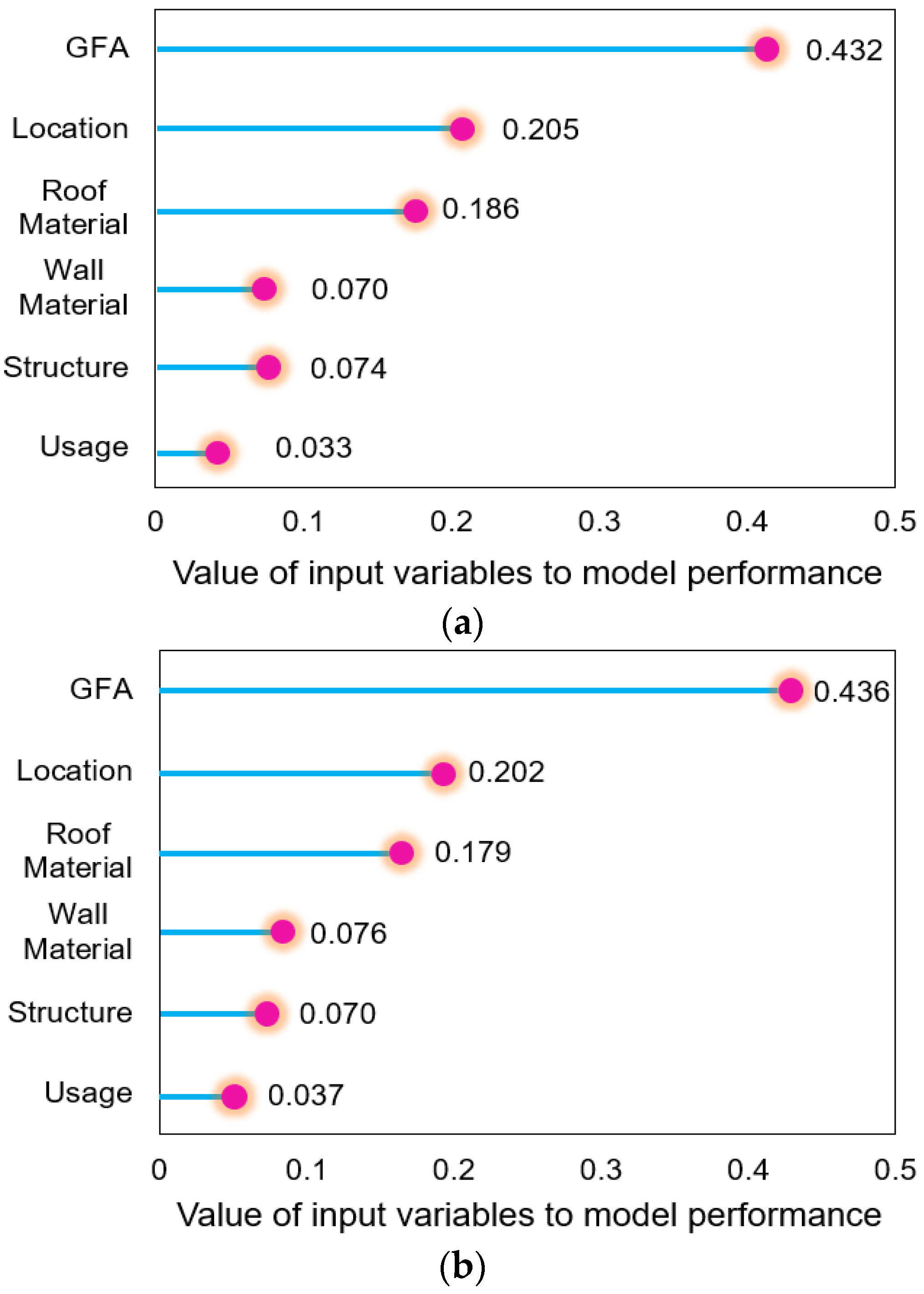
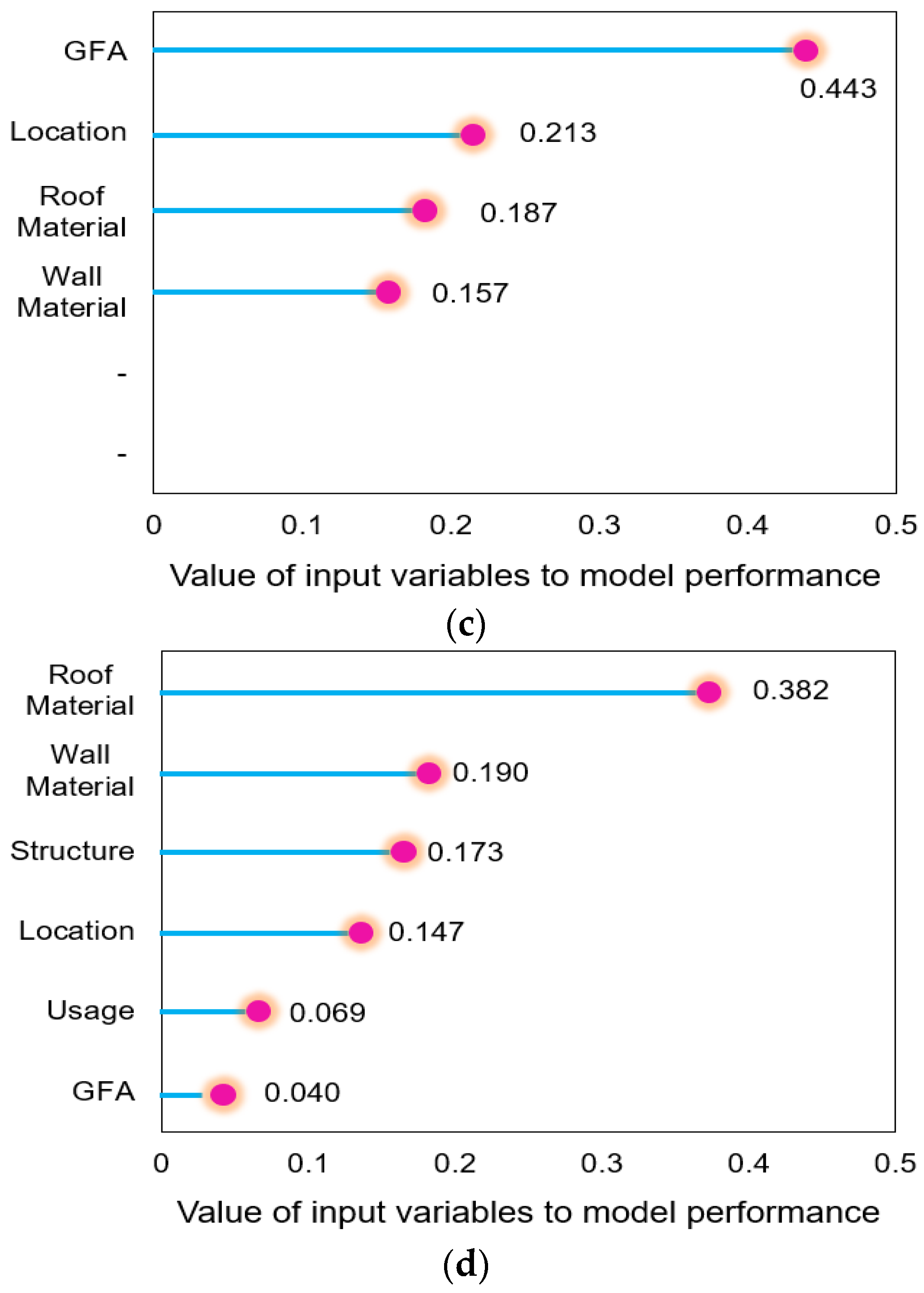
Six features—location, structure, usage, GFA, wall material, and roof material—were utilized to estimate DWGR, and a difference in the contribution of features affecting the performance of RF, ET, GBM, and XGboost predictive models was recorded. Figure 2a–d shows the feature importance analysis results of the models exhibiting the best predictive performance using the optimal estimator number for each RF, ET, GBM, and XGboost algorithm (6, 450; 6, 400; 4, 300; and 6, 400, respectively). For RF, the most influential feature on DWGR was GFA (0.432), while the feature importance of location, roof material, wall material, structure, and usage was 0.205, 0.186, 0.070, 0.074, and 0.033, respectively. For ET, GFA importance (0.436) was highest, while that of location, roof material, wall material, structure, and usage tended to be similar to that of RF. For the GBM model, the 4 feature (GFA, location, roof, and wall material) had the greatest impact on DWGR, and the feature importance of GFA was the highest at 0.443. Alternatively, the XGboost predictive model exhibited a different trend of feature importance from RF, ET, and GBM (Figure 2d). In the XGBoost predictive model, the most important feature on DWGR was roof material (0.382), followed by wall material, structure, location, usage, and GFA (0.190, 0.173, 0.147, 0.069, and 0.040, respectively). This finding notably contrasts others, with regards to GFA’s impact on DWGR in the three predictive models (i.e., RF, ET, and GBM). Accordingly, it was revealed that if even a specific feature plays an important role in numerous ML algorithms, its effect is in other models. Therefore, the application of suitable ML algorithms for data characteristics, and the development of proper features for various ML algorithms, are essential for developing ML models with optimal predictive performance.

3.3. Performance Evaluation and Optimal Ensemble Model

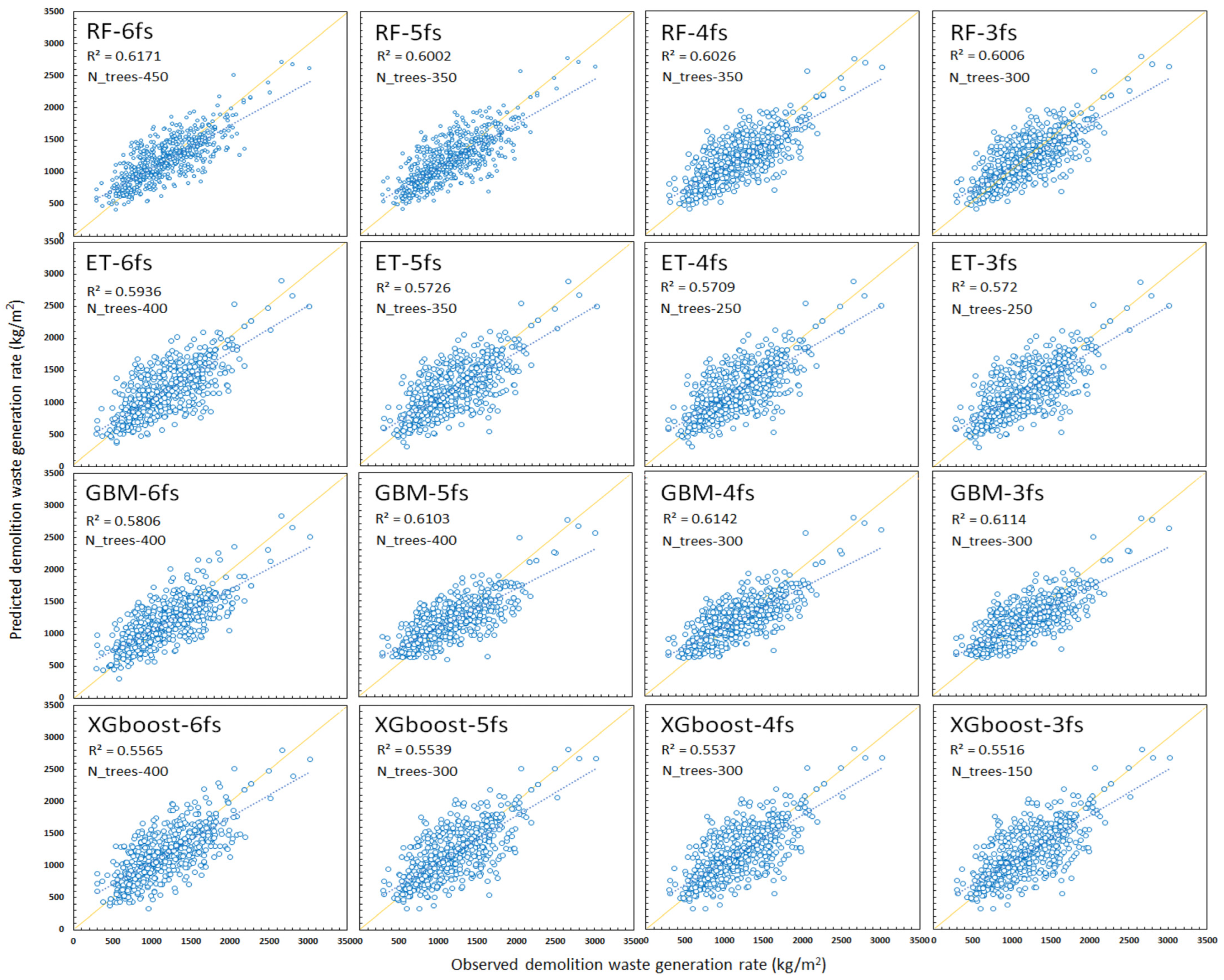
Figure 3 displays the correlation results according to the feature combinations of the four ensemble models for DWGR, and Table 5 shows the performance indicator results of the model having the optimal number of estimators. The RF model achieved the best predictive performance at the 6-feature level (RMSE, 253.727; R2, 0.6171; R, 0.7855), while the 3-feature predictive model produced the lowest prediction performance (RMSE, 261.836; R2, 0.6006; R, 0.7750). Similarly, in the ET and XGboost models, the best and worst predictive performances were achieved in the 6- and 3-feature predictive models, respectively. In contrast, the 4-feature predictive model (RMSE, 253.085; R2, 0.6142; R 0.7837) produced the best GBM model; whereas the 5-, 4-, and 3-feature predictive models produced similar results. Interestingly, the predictive performance of the 6-feature model was the lowest (RMSE, 265.834; R2, 0.5806; R, 0.7620). Further, the accuracy of the RF 6-feature model was best among the 16 ensemble models in terms of R2 and R values; however, the RMSE results showed that the GBM 4-feature predictive model with an RMSE value of 253.085 was slightly better than the RF 6-feature model (RMSE 253.727). In addition, the GBM 4-feature predictive model (R2, 0.6142; R, 0.7837), presented prediction performances close to the RF 6-feature model. Similarly to the above, the RF and GBM models were determined to exhibit better predictive performances than either ET and XGboost algorithms based on the RMSE, R2, and R performance evaluation results.
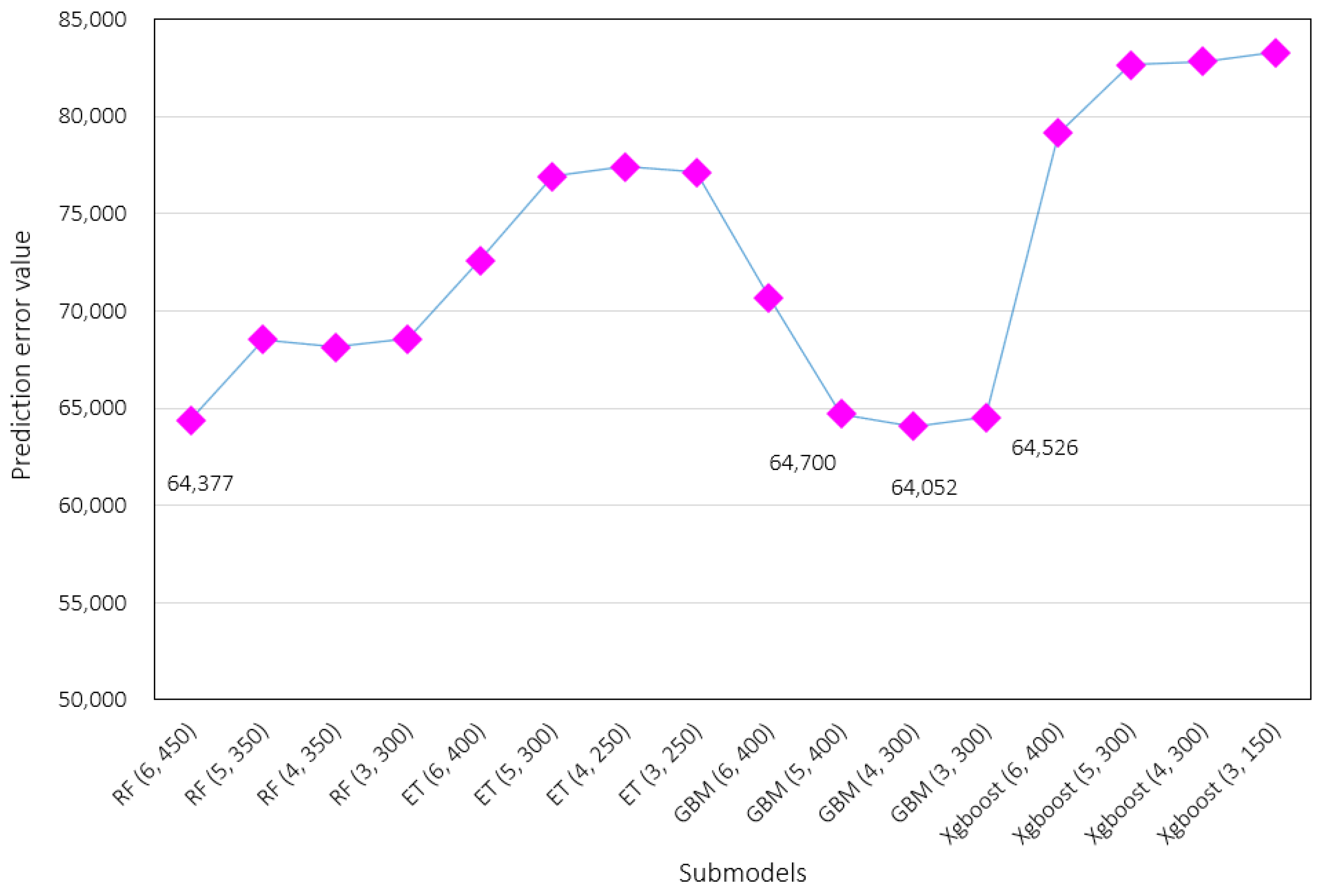
Model prediction error was also investigated to obtain the best variance–bias balance, together with the accuracy performance evaluation ensemble models (Figure 4). Since the prediction error of the GBM (4, 300) predictive model was the lowest (64,052), it was considered the best in terms of variance–bias tradeoff. The prediction errors of RF (6, 450), GBM (3, 300), and GBM (5, 400) models were 64,377, 64,526, and 64,700, respectively, notably similar to GBM (4, 300). Conversely, the prediction error was >72,574 and >79,122 for the ET and XGboost models. Accordingly, the GBM (4, 300), RF (6, 450), GBM (3, 300), and GBM (5, 400) predictive models were deemed the most appropriate model for achieving optimal variance–bias balance based on the prediction error.
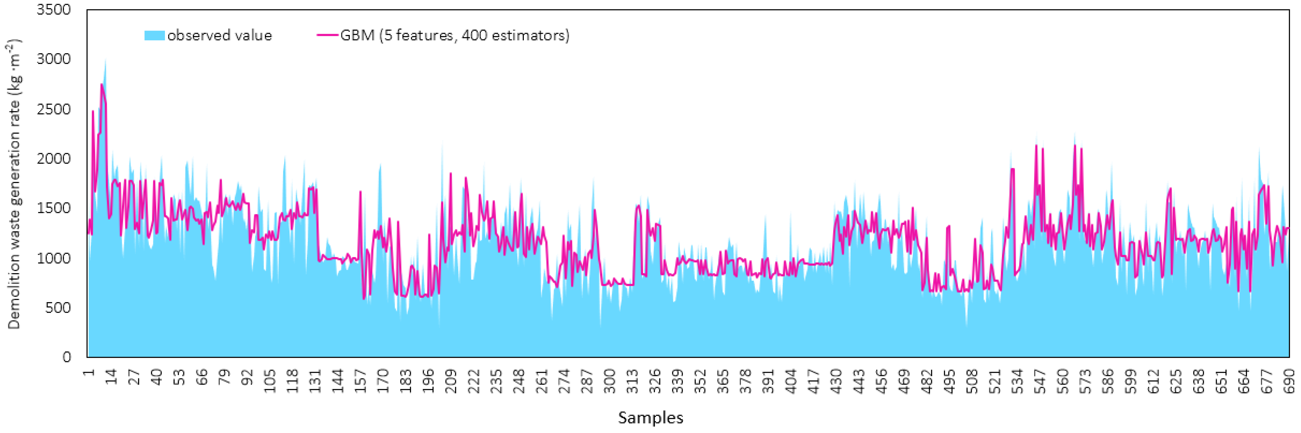
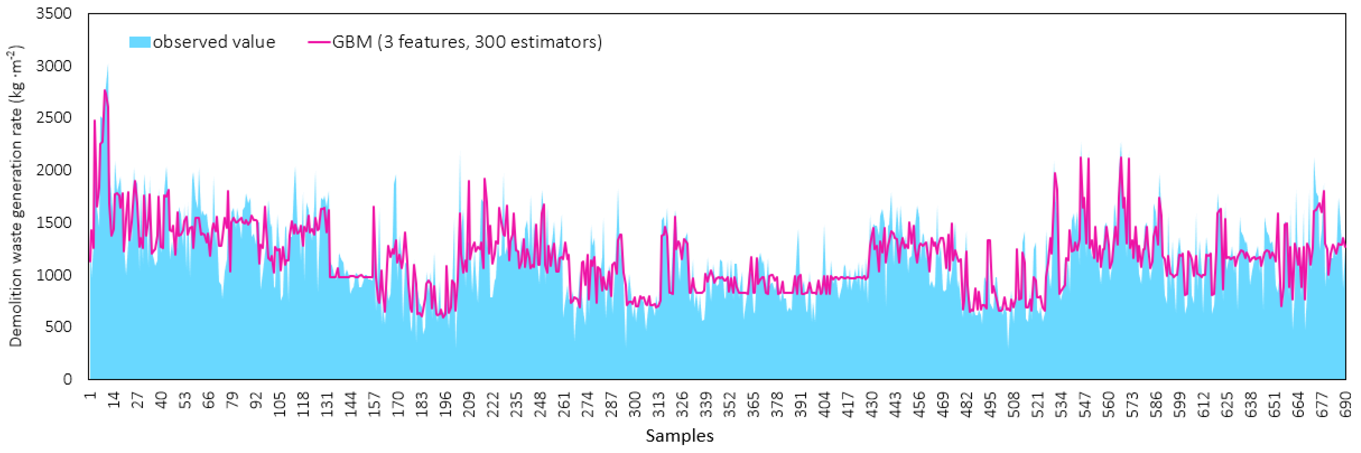
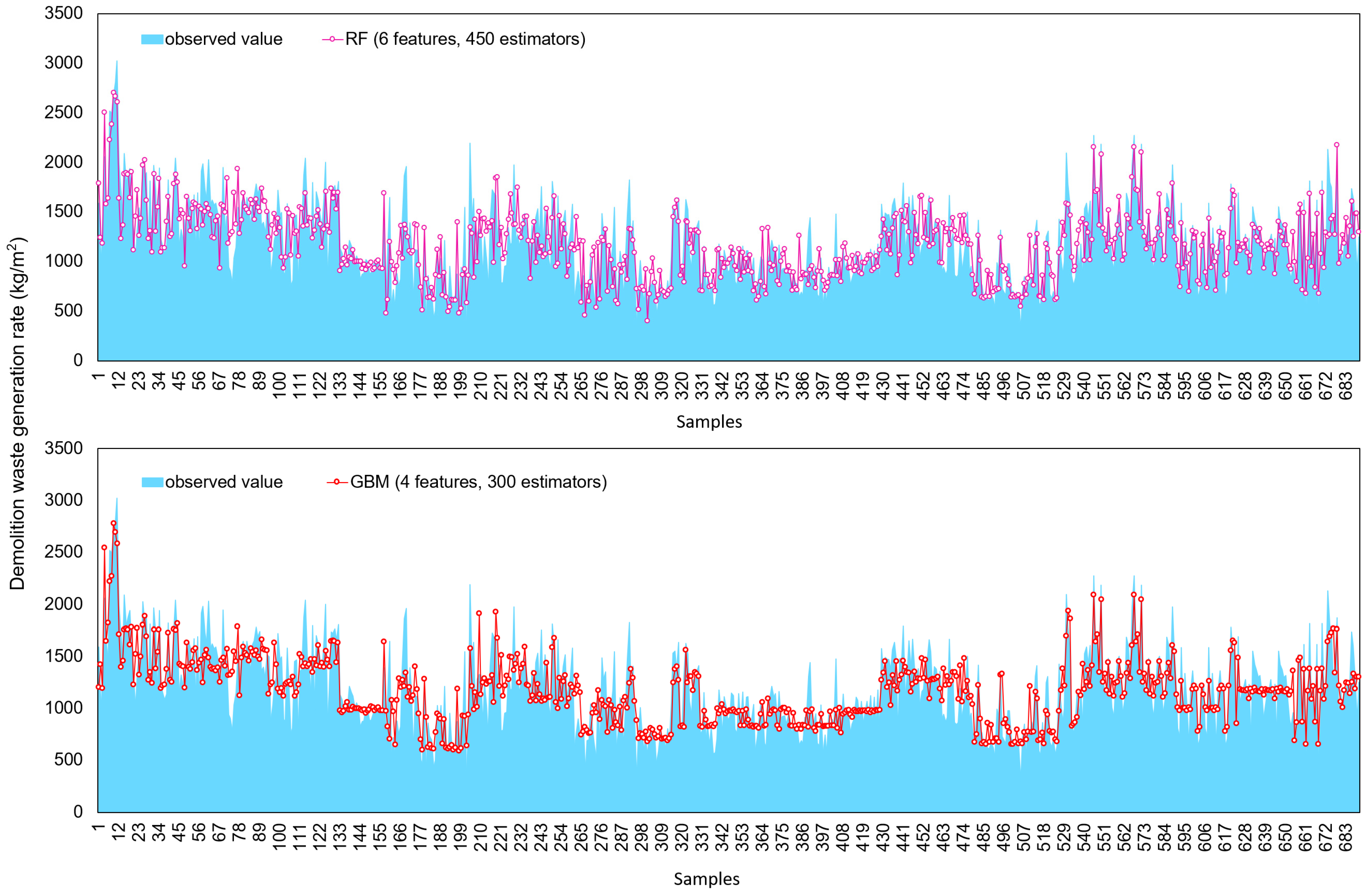
Combining the performance evaluation results of the ensemble models above, the RF (6, 450) predictive model was deemed the best model in terms of R2 and R values; whereas the GBM (4, 300) predictive model was best in terms of RMSE and prediction error. Accordingly, the RF (6, 450) and GBM (4, 300) predictive models were considered the most optimal for predicting DWGR (kg·m−2) based on the variable data of the five categorical and one numerical features. The observed and predicted values by the RF (6, 450) and GBM (4, 300) models are shown in Figure 5, where the mean observed value was 1171.2 kg·m−2, and the means of the RF (6, 450) and GBM (4, 300) models were 1169.94 and 1166.25 kg·m−2, respectively. The observed and predicted values by the GBM (3, 300), GBM (5, 400), ET (6, 400), and XGboost (6, 400) models are shown in Figure A1, Figure A2, Figure A3 and Figure A4.

4. Discussion

Building characteristics (e.g., GFA, usage, structure, location, etc.) were determined as the major key factors affecting DWGR [61]. Poon et al. [62] and Lu et al. [9] presented the correlation between GFA and DWGR, while Banias [63] that between usage and DWGR. Andersen et al. [64], Bergsdal et al. [65], and Bohne et al. [66] studied the effects of regional factors on DWGR; whereas the results of the present study indicated the highest feature importance of GFA and location for the developed RF, ET, and GBM models, in notable agreement with the existing research results (Figure 2a–d). Notably, the feature importance of wall and roof materials was higher than that of structure and usage in the present study; however, the wall and roof materials were not considered as major factors affecting DWGR in the previous studies. Further, the wall and roof materials exhibited higher feature importance than the GFA, usage, location, and structure in the XGboost model; accordingly, the feature importance of input variables in this model was quite different from that of the RT, ET, and GBM models, and there was a significant difference in the factors affecting DWGR from those presented in previous studies.
Section 2.3 presents a review of the existing research literature, and indicates that ET is an improved bagging method compared to RF in terms of bias and variance; whereas XGboost is a superior boosting method than GBM for accuracy improvement and overfitting prevention. The results of the predictive models employing the RF, ET, GBM, and XGboost ensemble algorithms in this study (Figure 3 and Figure 4; Table 5), however, were varied. The predictive performance of RF and GBM models in the present study was better than that of ET and XGboost models in terms of accuracy and prediction error. The existing research has employed DT-based ensemble algorithms [32], together with LightGBM, ET, RF, and Xgboost for time series datasets to estimate daily household waste generation. Specifically, Namoun et al. [32] found that LightGBM and ET algorithms exhibited better predictive performances than RF and XGboost. According to the results of a study applying a DT-based ensemble, except for C&D waste generation, Byeon [67] developed a predictive model to identify hypokinetic dysarthria by employing a DT classification and regression tree (CART), RF, GBM, and XGboost algorithms. The authors found that GBM (accuracy 83.1%) and RF (accuracy 83.8%) models achieved better predictive performances than the XGboost (accuracy 81.1%) and DT (accuracy 70.3%) models, where 16 input features (14 numerical, 2 categorical) were used. Ahmad et al. [68] used DT, ET, SVR, and RF to estimate useful solar thermal energy with 9 input features (8 numerical, 1 categorical), producing predictive performances (R2) of 0.957, 0.954, 0.930, and 0.903 for RF, ET, DT, and SVR, respectively, indicating the strength of the RF and ET models. Papadopoulos et al. [41] applied the GBM, RT, and ET algorithms using 8 numerical input features to estimate energy (cooling and heating) load, and revealed that the GBM model exhibited the best predictive performance in terms of mean square error (MSE) scores. In the case of heating load prediction, ET and RF produced similar results; whereas for the cooling load, ET was superior to RF.
Accordingly, previous studies using DT-based ensembles demonstrated various results regardless of the type of algorithms due to the difference in the characteristics of data used in each study (e.g., input feature types or sample size). Further, this may also be related to the considerable variation of the models’ predictive performances depending on the selection and adjustment of hyper-parameters before the algorithm applications in each study. Thus, the proper selection of algorithms and hyper-parameters in consideration of data characteristics are important issues during the development of ML models, and the process of deriving the optimal ML model in consideration of these issues becomes a key factor associated with predictive performance results. Considering these facts, this study developed an optimal ML model for predicting DWGR. To this end, a new set of input variables was developed, including the input variables used for DWGR prediction in previous studies [64,65,66]. In addition, this study applied DT-based algorithms considering the characteristics of the dataset and developed submodels applying various hyper-parameters. Based on this, a prediction model was developed with hyper-parameters for the final optimal performance model for DWGR prediction.

5. Conclusions

In this study, DT-based ensemble algorithms (i.e., RT, ET, GBM, and XGboost) were applied in consideration of data characteristics (relatively small-sized dataset consisting of categorical variables) to estimate DWGR (kg·m−2) in the end-of-life stage of a building. To develop a model, submodels were created according to the input features (GFA, location, usage, structure, wall materials, and roof materials), and the number of estimators. Subsequently, the optimal DT-based ensemble models were derived using performance indicators, such as R2, R, RMSE, and prediction error. The findings of this study are summarized as follows.
(1)
RF and GBM exhibited superior predictive performances compared to ET and XGboost for the relatively small, categorical data environment.
(2)
The most suitable models were RF (6 features, 450 trees) and GBM (4 features, 300 trees), where the predictive performance of the former was: R2, 0.6171; R, 0.7855; RMSE, 253.727; prediction error, 64,377; and latter was R2, 0.6142; R, 0.7837; RMSE, 253.085; and prediction error, 64,052. The mean observed value was 1171.2 kg·m−2, while the means of the RF (6, 450) and GBM (4, 300) models were 1169.94 and 1166.25 kg·m−2, respectively. The GBM model presented excellent performance, even with 3- and 5-features, or 300 and 400 estimators. The mean of the GBM (3, 300) and GBM (5, 400) predictive models was 1167.14 and 1165.22 kg·m−2, respectively.
(3)
A different result in feature importance was observed in the RT, ET, GBM, and XGboost models. In particular, the feature importance of GFA (0.432) had the greatest impact on RT, ET, and GBM models, followed by location, roof materials, and wall materials. For XGboost, the highest feature importance of 0.382 was determined to be the roof material, followed by wall material, structure, location, and usage; whereas the lowest feature importance was GFA.
The features used in this study correspond to the building exterior and characteristics that can be easily obtained from the building register provided by administrative agencies. This can facilitate decommissioning engineers or company officials for the rapid collection of applicable modeling features and is beneficial for benchmarking the DWGR predictive models here. In particular, the proposed GBM model could be employed to estimate DWGR, even with 4-features. Therefore, it was concluded that the proposed methods here can be easily used as a decision-making tool in demolition waste management plans for decommissioning engineers and companies.
As the model developed in this study was derived using a relatively small dataset, the limitation in ML modeling results due to dataset size was unavoidable. As the data used in this study referred to the field-collected values acquired through a direct survey before building demolition, future limitations in terms of time and manpower will be encountered. Thus, additional research should be conducted to derive a model that can improve accuracy through data collection methods such as surveys in future development. In addition, the performance of the model developed in this study can be seen as another limitation of this study that it is difficult to say that the R2 value has an excellent predictive performance of about 0.62. It is difficult to see this reason as a problem of the type of ML algorithm selected or data preprocessing technology, and it is judged that there is a high possibility that distortion of the collected data has occurred by the investigators who participated in the data collection. In this respect, it seems necessary to properly control the uncertainty problem caused by the data collection method, and it seems that various DWGR data collection methods should be applied to secure reliable data.

Author Contributions

Conceptualization, methodology, validation, and supervision, G.-W.C. and Y.-C.K.; Writing—original draft preparation, G.-W.C.; Formal analysis, G.-W.C.; Resources, writing—review, editing and funding acquisition, G.-W.C., Y.-C.K., W.-H.H. and S.-H.C. All authors have read and agreed to the published version of the manuscript.

Funding

This work was supported in part by the National Research Foundation of Korea (NRF) grants funded by the Korean Government (MSIT) [NRF-2019R1A2C1088446; NRF-2020R1C1C1009061].

Institutional Review Board Statement

Not applicable.

Informed Consent Statement

Not applicable.

Data Availability Statement

All data included in this study are available upon request by contact with the corresponding author.

Conflicts of Interest

The authors declare no conflict of interest.

Appendix A

Figure A1. GBM−5 features, 400 estimators.
Sustainability 15 10163 g0a1
Figure A2. GBM−3 features, 300 estimators.
Sustainability 15 10163 g0a2
Figure A3. ET−6 features, 400 estimators.
Sustainability 15 10163 g0a3
Figure A4. XGboost−6 features, 400 estimators.
Sustainability 15 10163 g0a4

References

  1. Leao, S.; Bishop, I.; Evans, D. Spatial–temporal model for demand and allocation of waste landfills in growing urban regions. Comput. Environ. Urban Syst. 2004, 28, 353–385. [Google Scholar] [CrossRef]
  2. Ekanayake, L.L.; Ofori, G. Building waste assessment score: Design-based tool. Build. Environ. 2004, 39, 851–861. [Google Scholar] [CrossRef]
  3. Huang, X.; Xu, X. Legal regulation perspective of eco-efficiency construction waste reduction and utilization. Urban Dev. Stud. 2011, 9, 90–94. [Google Scholar]
  4. Islam, R.; Nazifa, T.H.; Yuniarto, A.; Uddin, A.S.; Salmiati, S.; Shahid, S. An empirical study of construction and demolition waste generation and implication of recycling. Waste Manag. 2019, 95, 10–21. [Google Scholar] [CrossRef]
  5. Li, J.; Ding, Z.; Mi, X.; Wang, J. A model for estimating construction waste generation index for building project in China. Resour. Conserv. Recycl. 2013, 74, 20–26. [Google Scholar] [CrossRef]
  6. Llatas, C. A model for quantifying construction waste in projects according to the European waste list. Waste Manag. 2011, 31, 1261–1276. [Google Scholar] [CrossRef]
  7. Wang, J.; Li, Z.; Vivian Tam, W.Y. Identifying best design strategies for construction waste minimization. J. Clean. Prod. 2015, 92, 237–247. [Google Scholar] [CrossRef]
  8. Butera, S.; Christensen, T.H.; Astrup, T.F. Composition and leaching of construction and demolition waste: Inorganic elements and organic compounds. J. Hazard. Mater. 2014, 276, 302–311. [Google Scholar] [CrossRef]
  9. Lu, W.S.; Yuan, H.P. A framework for understanding waste management studies in construction. Waste Manag. 2011, 31, 1252–1260. [Google Scholar] [CrossRef] [Green Version]
  10. Song, Y.; Wang, Y.; Liu, F.; Zhang, Y. Development of a hybrid model to predict construction and demolition waste: China as a case study. Waste Manag. 2017, 59, 350–361. [Google Scholar] [CrossRef]
  11. Lu, W.; Yuan, H.; Li, J.; Hao, J.J.; Mi, X.; Ding, Z. An empirical investigation of construction and demolition waste generation rates in Shenzhen city, South China. Waste Manag. 2011, 31, 680–687. [Google Scholar] [CrossRef] [Green Version]
  12. Hurley, J.W. Valuing the Pre-Demolition Audit Process; CIB Rep.: Lake Worth, FL, USA, 2003; Volume 287, Available online: http://cibw117.com/europe/valuing-the-pre-demolition-audit-process/ (accessed on 22 November 2017).
  13. Jalali, G.Z.M.; Nouri, R.E. Prediction of municipal solid waste generation by use of artificial neural network: A case study of Mashhad Intern. J. Environ. Res. 2008, 2, 13–22. [Google Scholar]
  14. Milojkovic, J.; Litovski, V. Comparison of some ANN based forecasting methods implemented on short time series. In Proceedings of the 9th Symposium on Neural Network Applications in Electrical Engineering, Belgrade, Serbia, 25–27 September 2008; pp. 175–178. [Google Scholar]
  15. Noori, R.; Abdoli, M.A.; Ghazizade, M.J.; Samieifard, R. Comparison of neural network and principal component-regression analysis to predict the solid waste generation in Tehran. Iran. J. Public Health 2009, 38, 74–84. [Google Scholar]
  16. Patel, V.; Meka, S. Forecasting of municipal solid waste generation for medium scale towns located in the state of Gujarat, India. Int. J. Innov. Res. Sci. Engin. Technol. 2013, 2, 4707–4716. [Google Scholar]
  17. Noori, R.; Abdoli, M.A.; Ghasrodashti, A.A.; Ghazizade, M.J. Prediction of municipal solid waste generation with combination of support vector machine and principal component analysis: A case study of Mashhad. Environ. Prog. Sustain. Energy 2008, 28, 249–258. [Google Scholar] [CrossRef]
  18. Dai, C.; Li, Y.P.; Huang, G.H. A two-stage support-vector-regression optimization model for municipal solid waste management–a case study of Beijing, China. J. Environ. Manag. 2011, 92, 3023–3037. [Google Scholar] [CrossRef]
  19. Abdoli, M.A.; Nezhad, M.F.; Sede, R.S.; Behboudian, S. Longterm forecasting of solid waste generation by the artificial neural networks. Environ. Prog. Sustain. Energy 2011, 31, 628–636. [Google Scholar] [CrossRef]
  20. Afon, A.O.; Okewole, A. Estimating the quantity of solid waste generation in Oyo, Nigeria. Waste Manag. Res. 2007, 25, 371–379. [Google Scholar] [CrossRef]
  21. Thanh, N.P.; Matsui, Y.; Fujiwara, T. Household solid waste generation and characteristic in a Mekong Delta city, Vietnam. J. Environ. Manag. 2010, 91, 2307–2321. [Google Scholar] [CrossRef]
  22. Yuan, A.O.; Wu, C.; Huang, Z.W. The prediction of the output of municipal solid waste (MSW) in Nanchong city. Adv. Mater. Res. 2012, 518–523, 3552–3556. [Google Scholar] [CrossRef]
  23. Kontokosta, C.E.; Hong, B.; Johnson, N.E.; Starobin, D. Using machine learning and small area estimation to predict building-level municipal solid waste generation in cities. Comput. Environ. Urb. Syst. 2018, 70, 151–162. [Google Scholar] [CrossRef]
  24. Akanbi, L.A.; Oyedele, A.O.; Oyedele, L.O.; Salami, R.O. Deep learning model for demolition waste prediction in a circular economy. J. Clean. Prod. 2020, 274, 122843. [Google Scholar] [CrossRef]
  25. Nguyen, X.C.; Nguyen, T.T.H.; La, D.D.; Kumar, G.; Rene, E.R.; Nguyen, D.D.; Nguyen, V.K. Development of machine learning-based models to forecast solid waste generation in residential areas: A case study from Vietnam. Res. Conserv. Recycl. 2021, 167, 105381. [Google Scholar] [CrossRef]
  26. Jayaraman, V.; Parthasarathy, S.; Lakshminarayanan, A.R.; Singh, H.K. Predicting the quantity of municipal solid waste using XGBoost model. In Proceedings of the 3rd International Conference on Inventive Research in Computing Applications (ICIRCA), Coimbatore, India, 2–4 September 2021; pp. 148–152. [Google Scholar]
  27. Johnson, N.E.; Ianiuk, O.; Cazap, D.; Liu, L.; Starobin, D.; Dobler, G.; Ghandehari, M. Patterns of waste generation: A gradient boosting model for short-term waste prediction in New York City. Waste Manag. 2017, 62, 3–11. [Google Scholar] [CrossRef] [PubMed]
  28. Kumar, A.; Samadder, S.R.; Kumar, N.; Singh, C. Estimation of the generation rate of different types of plastic wastes and possible revenue recovery from informal recycling. Waste Manag. 2018, 79, 781–790. [Google Scholar] [CrossRef]
  29. Kannangara, M.; Dua, R.; Ahmadi, L.; Bensebaa, F. Modeling and prediction of regional municipal solid waste generation and diversion in Canada using machine learning approaches. Waste Manag. 2018, 74, 3–15. [Google Scholar] [CrossRef]
  30. Lu, W.; Lou, J.; Webster, C.; Xue, F.; Bao, Z.; Chi, B. Estimating construction waste generation in the Greater Bay Area, China using machine learning. Waste Manag. 2021, 134, 78–88. [Google Scholar] [CrossRef]
  31. Ghanbari, F.; Kamalan, H.; Sarraf, A. An evolutionary machine learning approach for municipal solid waste generation estimation utilizing socioeconomic components Arab. J. Geosci. 2021, 14, 92. [Google Scholar]
  32. Namoun, A.; Hussein, B.R.; Tufail, A.; Alrehaili, A.; Syed, T.A.; BenRhouma, O. An ensemble learning based classification approach for the prediction of household solid waste generation. Sensors 2022, 22, 3506. [Google Scholar] [CrossRef]
  33. da Figueira, A.; Pitombo, C.S.; de Oliveira, P.T.M.e.S.; Larocca, A.P.C. Identification of rules induced through decision tree algorithm for detection of traffic accidents with victims: A study case from Brazil. Case Stud. Transp. Polic. 2017, 5, 200–207. [Google Scholar] [CrossRef]
  34. Pal, M.; Mather, P.M. An assessment of the effectiveness of decision tree methods for land cover classification. Remote Sens. Env. 2003, 86, 554–565. [Google Scholar] [CrossRef]
  35. Brown, G. Ensemble Learning. In Encyclopedia of Machine Learning and Data Mining; Sammut, C., Webb, G.I., Eds.; US Springer: New York, NY, USA, 2017; pp. 393–402. [Google Scholar]
  36. Krogh, A.; Vedelsby, J. Neural network ensembles, cross validation, and active learning. Adv. Neural Inf. Process. Syst. 1995, 7, 231–238. [Google Scholar]
  37. Perrone, M.P.; Cooper, L.N. When networks disagree: Ensemble methods for hybrid neural networks. In How We Learn; How We Remember: Toward an Understanding of Brain and Neural Systems: Selected Papers of Leon N Cooper; World Scientific: Singapore, 1992. [Google Scholar]
  38. Dietterich, T.G. Ensemble methods in machine learning. In International Workshop on Multiple Classifier Systems; Springer: Berlin/Heidelberg, Germany, 2000; pp. 1–15. [Google Scholar]
  39. Breiman, L. Random forests. Mach. Learn. 2001, 45, 5–32. [Google Scholar] [CrossRef] [Green Version]
  40. Geurts, P.; Ernst, D.; Wehenkel, L. Extremely randomized trees. Mach. Learn. 2006, 63, 3–42. [Google Scholar] [CrossRef] [Green Version]
  41. Papadopoulos, S.; Azar, E.; Woon, W.L.; Kontokosta, C.E. Evaluation of tree-based ensemble learning algorithms for building energy performance estimation. J. Build. Perform. Simul. 2018, 11, 322–332. [Google Scholar] [CrossRef]
  42. Friedman, J.H. Stochastic gradient boosting. Comp. Stat. Data Anal. 2002, 38, 367–378. [Google Scholar] [CrossRef]
  43. Fan, J.; Yue, W.; Wu, L.; Zhang, F.; Cai, H.; Wang, X.; Xiang, Y. Evaluation of SVM, ELM and four tree-based ensemble models for predicting daily reference evapotranspiration using limited meteorological data in different climates of China. Agric. Forest Meteorol. 2018, 263, 225–241. [Google Scholar] [CrossRef]
  44. Chen, T.; Guestrin, C. Xgboost: A scalable tree boosting system. In Proceedings of the 22nd ACM SIGKDD International Conference on Knowledge Discovery and Data Mining, San Francisco, CA, USA, 13–17 August 2016; pp. 785–794. [Google Scholar]
  45. Le, L.T.; Nguyen, H.; Zhou, J.; Dou, J.; Moayedi, H. Estimating the heating load of buildings for smart city planning using a novel artificial intelligence technique PSO-XGBoost. Appl. Sci. 2019, 9, 2714. [Google Scholar] [CrossRef] [Green Version]
  46. Qiu, Y.; Zhou, J.; Khandelwal, M.; Yang, H.; Yang, P.; Li, C. Performance evaluation of hybrid WOA-XGBoost, GWO-XGBoost and BO-XGBoost models to predict blast-induced ground vibration. Eng. Comput. 2021, 38, 4145–4162. [Google Scholar] [CrossRef]
  47. Zhou, J.; Qiu, Y.; Khandelwal, M.; Zhu, S.; Zhang, X. Developing a hybrid model of Jaya algorithm-based extreme gradient boosting machine to estimate blast-induced ground vibrations Intern. J. Rock Mech. Min. Sci. 2021, 145, 104856. [Google Scholar] [CrossRef]
  48. Zhou, J.; Qiu, Y.; Zhu, S.; Armaghani, D.J.; Khandelwal, M.; Mohamad, E.T. Estimation of the TBM advance rate under hard rock conditions using XGBoost and Bayesian optimization. Undergr. Space 2021, 6, 506–515. [Google Scholar] [CrossRef]
  49. Farooq, F.; Ahmed, W.; Akbar, A.; Aslam, F.; Alyousef, R. Predictive modeling for sustainable high-performance concrete from industrial wastes: A comparison optimization of models using ensemble learners. J. Clean. Prod. 2021, 292, 126032. [Google Scholar] [CrossRef]
  50. Chen, K.; Peng, Y.; Lu, S.; Lin, B.; Li, X. Bagging based ensemble learning approaches for modeling the emission of PCDD/Fs from municipal solid waste incinerators. Chemosphere 2021, 274, 129802. [Google Scholar] [CrossRef]
  51. Probst, P.; Boulesteix, A.L. To tune or not to tune the number of trees in random forest. J. Mach. Learn. Res. 2017, 18, 6673–6690. [Google Scholar]
  52. Cheng, J.; Dekkers, J.C.; Fernando, R.L. Cross-validation of best linear unbiased predictions of breeding values using an efficient leave-one-out strategy. J. Anim. Breed. Genet. 2021, 138, 519–527. [Google Scholar] [CrossRef]
  53. Wong, T.T. Performance evaluation of classification algorithms by K-fold and leave-one-out cross validation. Pattern Recog. 2015, 48, 2839–2846. [Google Scholar] [CrossRef]
  54. Witten, I.H.; Frank, E.; Hall, M.A. Data Mining: Practical Machine Learning Tools and Techniques, 3rd ed.; Morgan Kaufmann: Burlington, MA, USA, 2011. [Google Scholar]
  55. Cha, G.W.; Moon, H.J.; Kim, Y.M.; Hong, W.H.; Hwang, J.H.; Park, W.J.; Kim, Y.C. Development of a prediction model for demolition waste generation using a random forest algorithm based on small datasets Intern. J. Environ. Res. Public Health 2020, 17, 6997. [Google Scholar] [CrossRef]
  56. Cha, G.W.; Moon, H.J.; Kim, Y.C. Comparison of random forest gradient boosting machine models for predicting demolition waste based on small datasets categorical variables Intern. J. Environ. Res. Public Health 2021, 18, 8530. [Google Scholar] [CrossRef]
  57. Cheng, H.; Garrick, D.J.; Fernando, R.L. Efficient strategies for leave-one-out cross validation for genomic best linear unbiased prediction. J. Anim. Sci. Biotechnol. 2017, 8, 38. [Google Scholar] [CrossRef] [Green Version]
  58. Shao, Z.; Er, M.J. Efficient leave-one-out cross-validation-based regularized extreme learning machine. Neurocomputing 2016, 194, 260–270. [Google Scholar] [CrossRef]
  59. Shahhosseini, M.; Hu, G.; Pham, H. Optimizing ensemble weights and hyperparameters of machine learning models for regression problems. Mach. Learn. Appl. 2022, 7, 100251. [Google Scholar] [CrossRef]
  60. Hastie, T.; Tibshirani, R.; Friedman, J.; Franklin, J. The elements of statistical learning: Data mining, inference and prediction. Math. Intell. 2005, 27, 83–85. [Google Scholar]
  61. Chen, X.; Lu, W. Identifying factors influencing demolition waste generation in Hong Kong. J. Clean. Prod. 2017, 141, 799–811. [Google Scholar] [CrossRef] [Green Version]
  62. Poon, C.S.; Ann, T.W.; Ng, L.H. On-site sorting of construction and demolition waste in Hong Kong. Res. Conserv. Recycl. 2001, 32, 157–172. [Google Scholar] [CrossRef]
  63. Banias, G.; Achillas, C.; Vlachokostas, C.; Moussiopoulos, N.; Papaioannou, I. A web-based decision support system for the optimal management of construction and demolition waste. Waste Manag. 2011, 31, 2497–2502. [Google Scholar] [CrossRef]
  64. Andersen, F.M.; Larsen, H.; Skovgaard, M.; Moll, S.; Isoard, S. A European model for waste and material flows. Res. Conserv. Recycl. 2007, 49, 421–435. [Google Scholar] [CrossRef]
  65. Bergsdal, H.; Bohne, R.A.; Brattebø, H. Projection of construction and demolition waste in Norway. J. Ind. Ecol. 2007, 11, 27–39. [Google Scholar] [CrossRef]
  66. Bohne, R.A.; Brattebø, H.; Bergsdal, H. Dynamic eco-efficiency projections for construction and demolition waste recycling strategies at the city level. J. Ind. Ecol. 2008, 12, 52–68. [Google Scholar] [CrossRef]
  67. Byeon, H. Comparing ensemble-based machine learning classifiers developed for distinguishing hypokinetic dysarthria from presbyphonia. Appl. Sci. 2021, 11, 2235. [Google Scholar] [CrossRef]
  68. Ahmad, M.W.; Reynolds, J.; Rezgui, Y. Predictive modelling for solar thermal energy systems: A comparison of support vector regression random forest extra trees regression trees. J. Clean. Prod. 2018, 203, 810–821. [Google Scholar] [CrossRef]
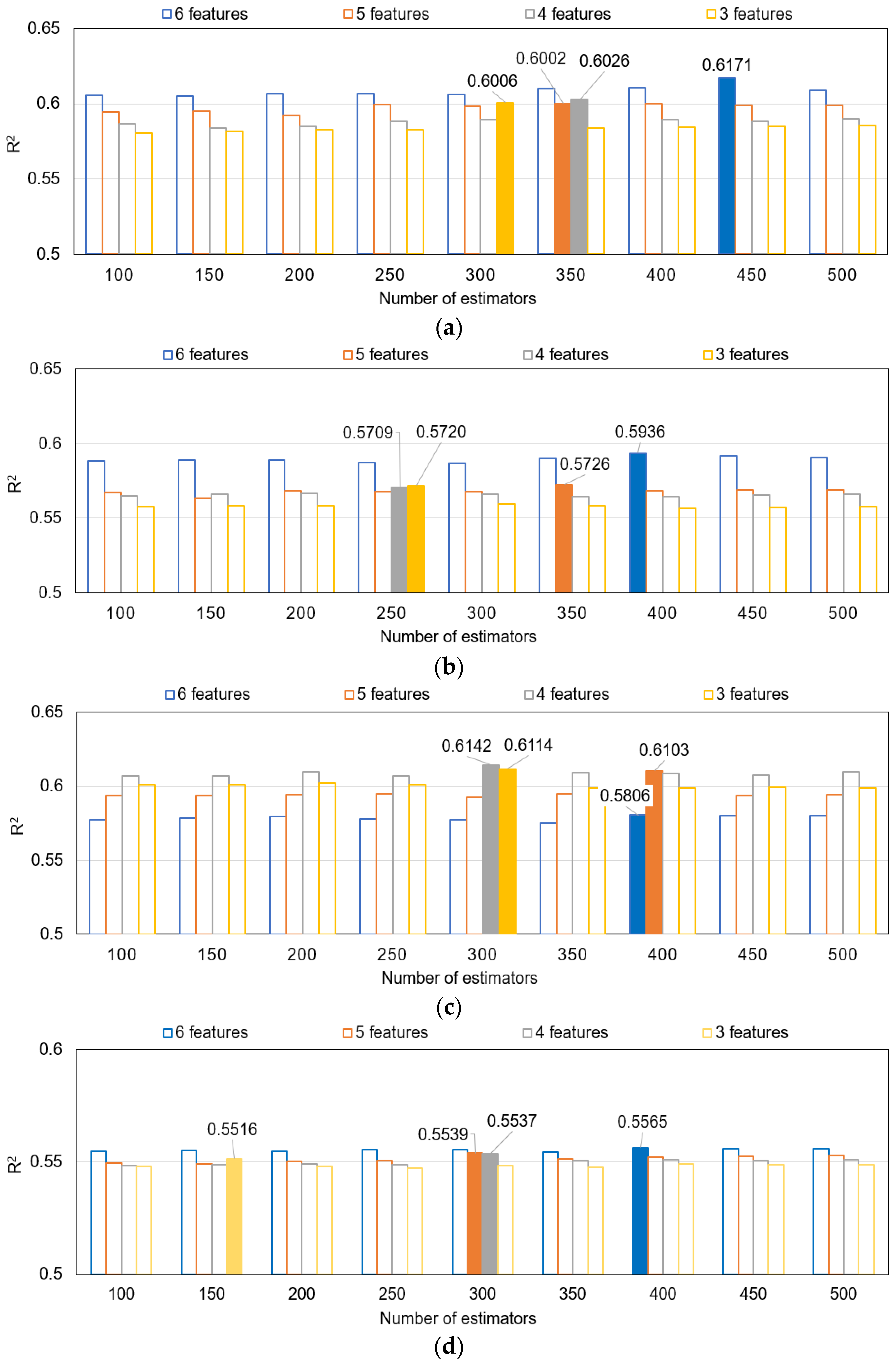
Figure 1. (a) R2 values according to number of estimators and features of RF model. (b) R2 values according to number of estimators and features of ET model. (c) R2 values according to number of estimators and features GBM model. (d) R2 values according to number of estimators and features of XGboost model.
Sustainability 15 10163 g001
Figure 2. (a) Feature importance of RFmodel with optimal numbers of features and estimators. (b) Feature importance of ET model with optimal numbers of features and estimators. (c) Feature importance of GBM model with optimal numbers of features and estimators. (d) Feature importance of XGboost model with optimal numbers of features and estimators.
Sustainability 15 10163 g002aSustainability 15 10163 g002b
Figure 3. Correlation between observed and predicted values according to the number of features of ensemble models. (The yellow line means the ideal line where the predicted value and the observed value are the same. The blue dotted line represents the R2 value).
Sustainability 15 10163 g003
Figure 4. Comparison of model prediction error values by variance–bias tradeoff.
Sustainability 15 10163 g004
Figure 5. Comparison of the observed and predicted DWGRs of RF (6 feature, 450 estimator) and GBM (4 feature, 300 estimator) models proposed as best.
Sustainability 15 10163 g005
Table 1. ML models applied to predict waste generation in previous studies.
StudiesWaste TypeApplied AlgorithmPerformance
Song et al. [10]C&D wasteGM-SVRthe average value of relative percent error < 0.1
Johnson et al. [27]MSWGBMR2 value: 0.685–0.906
Kontokosta et al. [23]MSWGBMR2 value: 0.73–0.87
Kumar et al. [28]MSWANNR2 value: 0.75
RFR2 value: 0.66
SVMR2 value: 0.74
Kannangara et al. [29]MSWANNR2 value: 0.72
DTR2 value: 0.54
PaperANNR2 value: 0.31
DTR2 value: 0.35
Lu et al. [30]C&D wasteGMR2 value: 0.977
ANNR2 value: 0.918
MLRR2 value: 0.777
DTR2 value: 0.764
Akanbi et al. [24]C&D wasteDNNR2 value: 0.948–0.994
Ghanbari et al. [31]MSWMultivariate adaptive regression splines (MARS)R2 value: 0.90
ANNR2 value: 0.74
RFR2 value: 0.88
Nguyen et al. [25]MSWKNNR2 value: 0.96
RFR2 value: 0.97
DNNR2 value: 0.91
Jayaraman et al. [26]MSWARIMAR2 value: −0.89
XGboostR2 value: 0.41
Namoun et al. [32]Household wasteSVRR2 value: 0.692
XGboostR2 value: 0.67
LightGBMR2 value: 0.745
RFR2 value: 0.714
ETR2 value: 0.737
ANNR2 value: 0.685
Table 2. Building status and statistical analysis of raw data used in this study.
CategoryNumbersGFA (m2)DWGR (kg·m−2)
TotalMinMeanMaxTotalMinMeanMax
Location134331,5422192275450,31029813136034
235640,653191141127485,0378313628574
38313,85126167414101,53173612231808
Usage159554,9291992514767,5788312908574
217228,706221671127251,38141814625718
31524102816179019,51060713012474
Structure18720,783472391127169,53841819496034
260456,9751994688788,0428313058574
3918288249120680,8892988892237
Wall material19369348410112710,35787111514696
223632,58423138790391,25925216586034
350047,0891994688596,7998311948574
4372679247213740,05651710832591
Roof material128943,565211511127479,35625216596034
23344147613428238,87725211781808
317812,4392370206227,92330612808574
428225,6271991688292,3148310372527
Location: 1—Project A, 2—Project B, 3—Project C. Structure: 1—Reinforced concrete (RC), 2—Masonry, 3—Wood. Usage: 1—Residential, 2—Residential and commercial, 3—Commercial. Wall material: 1—Concrete, 2—Brick, 3—Block, 4—Mud plastered and mortar wall. Roof material: 1—Slab, 2—Slab and roofing tile, 3—Slate, 4—Roofing tile.
Table 3. Changes in DWGR (kg·m−2) data statistics before and after data preprocessing.
Data PreprocessingNumber of SamplesMinimumMaximumAverageMedianStandard DeviationVariance
Before78283.34 8573.791327.971162.25809.2654,032.4
After690298.303024.041165.041138.30407.7166,016.7
Table 4. Hyper-parameters applied in ensemble model development for DWGR prediction.
AlgorithmHyper-ParameterDefinitionTested Value
RFn_estimatorsThe number of trees in the forest100, 150, 200, 250, 300, 350, 400, 450, 500
min_samples_splitThe minimum number of samples required to split an internal node1, 2, 3, 4, 5
min_samples_leafThe minimum number of samples required to be at a leaf node1, 2, 3, 4, 5
max_depthThe maximum depth of the treeMaximum possible
ETn_estimatorsThe minimum number of samples required to split an internal node100, 150, 200, 250, 300, 350, 400, 450, 500
min_samples_splitThe minimum number of samples required to be at a leaf node1, 2, 3, 4, 5
min_samples_leaf 1, 2, 3, 4, 5
max_depthThe maximum depth of the treeNone
max_leaf_nodes None
GBMn_estimatorsThe number of boosting stages100, 150, 200, 250, 300, 350, 400, 450, 500
min_samples_splitThe minimum number of samples required to split an internal node1, 2, 3, 4, 5
lossLeast squaresLeast squares
learning rateAmount of learning0.01, 0.1, 1
subsampleRate of sampling data to control overfitting1.0
XGboostn_estimatorsThe minimum number of samples required to split an internal node100, 150, 200, 250, 300, 350, 400, 450, 500
eta0.3 step size shrinkage used in update to prevent overfitting0.3
max_depthThe maximum depth of the tree10
min_child_weight 1
max_delta_step 0
subsample 1
Table 5. Comparison of model performance by RMSE, R2, and R.
Modeln_Featuren_EstimatorRMSER SquareR
RF6450253.7270.61710.7855
5350261.7720.60020.7747
4350260.9890.60260.7763
3300261.8360.60060.7750
ET6400269.3960.59360.7704
5350277.3340.57260.7567
4250278.2210.57090.7556
3250277.6900.57200.7563
GBM6400265.8340.58060.7620
5400254.3620.61030.7812
4300253.0850.61420.7837
3300254.0200.61140.7819
XGboost6400281.2620.55650.7460
5300287.4800.55390.7442
4300287.7900.55370.7441
3150288.5900.55160.7427
Disclaimer/Publisher’s Note: The statements, opinions and data contained in all publications are solely those of the individual author(s) and contributor(s) and not of MDPI and/or the editor(s). MDPI and/or the editor(s) disclaim responsibility for any injury to people or property resulting from any ideas, methods, instructions or products referred to in the content.