Spatial Distribution of Soil Heavy Metal Concentrations in Road-Neighboring Areas Using UAV-Based Hyperspectral Remote Sensing and GIS Technology

Abstract

Monitoring and restoring soil quality in areas neighboring roads affected by traffic activities require a thorough investigation of heavy metal concentrations. This study examines the spatial heterogeneity of copper (Cu) and chromium (Cr) concentrations in a 0.113 km² area adjacent to Jin-Long Avenue in Wuhan, China, using Unmanned Aerial Vehicle (UAV)-based hyperspectral remote sensing technology. Through this UAV-based remote sensing technology, we innovatively achieve a small-scale and fine-grained analysis of soil heavy metal pollution related with traffic activities, which represents a major contribution of this research study. In our approach, we generated 4375 spectral variates by transforming the original spectrum. To enhance result accuracy, we applied the Boruta algorithm and correlation analysis to select optimal spectral variates. We developed the retrieval model using the Gradient Boosting Decision Tree (GBDT) regression method, selected from a set of four regression methods using the LOOCV method. The resulting model yielded R-square values of 0.325 and 0.351 for Cu and Cr, respectively, providing valuable insights into the heavy metal concentrations. Based on the retrieved heavy metal concentrations from bare soil pixels (17,420 points), we analyzed the relationship between heavy metal concentrations and the perpendicular distance from the road. Additionally, we employed the universal kriging interpolation method to map heavy metal concentrations across the entire area. Our findings reveal that the concentration of heavy metals in this area exceeds background values and decreases as the distance from the road increases. This research significantly contributes to the understanding of spatial distribution characteristics and pollution caused by heavy metal concentrations resulting from traffic activities.

1. Introduction

Heavy metals (HMs) can enter the soil through various processes, such as industry, agriculture, and transportation, causing significant health risks to both humans and animals [1,2]. As per previous studies, transportation greatly contributes to soil heavy metal pollution [3,4,5]. Reports suggest that vehicle emissions, fossil fuel combustion, brake lining wear, and tire wear can contaminate the soil with lead (Pb), zinc (Zn), copper (Cu), chromium (Cr), and cadmium (Cd) [6,7]. Transportation-related dust containing HMs can combine with other airborne particles and enter the soil in a range of ways, such as deposition, dilution, diffusion, or attenuation. The soil near roads can have a heavy metal buildup due to transportation-related activities [8,9,10].

A study conducted in southeastern Iran assessed the heavy metal pollution in urban soils around industrial areas using samples and GIS technology. The results revealed several hot-spot areas with high concentrations of heavy metals, primarily associated with vehicle-related workshops, fuel stations, and road junctions [5]. Moreover, it has been identified that traffic flow contributes to increased lead (Pb) concentrations in surface soil [11]. Additionally, previous studies on heavy metals (HMs) related to traffic projects have shown that they tend to accumulate in the surface layer of soil on both sides of the road within a range of 20 cm. Notably, lead (Pb) and cadmium (Cd) exhibit a banded extension from the center of the road to the sides [12,13]. Another study, based on soil and earthworm samples from roadsides in urban high traffic areas in Benin Metropolis, Nigeria, also demonstrated a concentrated pattern of heavy metal pollution near roadsides, which gradually decreases with distance from the road [14]. It is important to note that the distribution of heavy metals varies across different regions and even within the same region [13]. However, existing works typically rely on traditional methods that involve soil sampling and laboratory analysis, which may not provide sufficient data density for local-level analysis on a fine spatial scale [5,14,15,16,17]. In light of these limitations, our study aims to conduct a spatially detailed analysis of heavy metal pollution, specifically chromium (Cr) and copper (Cu), in the road-neighboring area at a local scale. To achieve this objective, we will utilize UAV-based hyperspectral remote sensing technology.

In contrast to the traditional on-site soil sampling method [18,19], the hyper-spectral remote sensing technology uses hundreds of spectral bands and can capture detailed spectral characteristics of HMs and has been demonstrated to be an effective tool for estimating HM concentrations spatially in soil. It, thus, enables the study of the spatial distribution characteristics of heavy metals in soil with high precision and cost-effectiveness [18,19]. Most of the existing works based on hyperspectral remote sensing were carried out on spectroscopic reflectance and space-borne and air-borne hyperspectral methods [20]. Unmanned Aerial Vehicles (UAVs) equipped with hyperspectral sensors have been recently used for soil indicator monitoring due to their rapidness and convenience [21,22,23]. UAV-based remote sensing can monitor soil heavy metal concentration in much finer detail (submeter scale), benefiting the illustration of the mechanisms of the soil HM concentrations accumulation in a small area of interest, such as a small patch of farmland.

The main steps in hyperspectral remote sensing-based heavy metal retrieval are feature band selection and retrieval model building. As hyperspectral sensors have a large number of bands, the spectral variables usually have high dimensions, and projecting them through feature band selection methods into lower dimensions can lead to models with better generalization ability [24]. In terms of the retrieval model, both classical statistical regression models, such as linear regression [25], stepwise multiple linear regression (SMLR) [26], and partial least squares regression (PLSR) [27,28], and recently popular machine learning regression methods [29] are utilized in this field [30,31].

As mentioned earlier, our study aims to conduct a detailed spatial analysis of heavy metal pollution (specifically Cr and Cu) in a small soil area adjacent to a road at a submeter scale, using UAV-based hyperspectral technology, which provides higher spatial density data on heavy metal concentrations compared to on-site soil samples. The research consists of two parts: retrieving the heavy metal concentrations and analyzing their spatial distribution over the study area. In the first part, we will perform spectrum transformation, select optimal spectral variates, choose the best model, and retrieve heavy metal concentrations over bare soil points. In the second part, the study will analyze the spatial distribution and patterns of heavy metal concentrations. Additionally, it will examine the relationship between heavy metal concentrations at these points and their distance from the road. Summarily, this work represents an innovative way to analyze the spatial distribution characteristics of heavy metals at a submeter scale. It will also help identify the impact of traffic activities on the area adjacent to the road, which is challenging to illustrate based on limited on-site soil samples. The findings from this study will contribute to soil quality protection.

Following this introduction and background section, Section 2 talks about the study area, relevant data, and processing steps. The methodology used to retrieve heavy metal concentrations from hyperspectral data and analyze the spatial characteristic in the subsequent sections of the paper. Thereafter, the results are presented and analyzed. Finally, the paper concludes with a summary of key findings, limitations, and recommendations.

2. Study Area and Materials

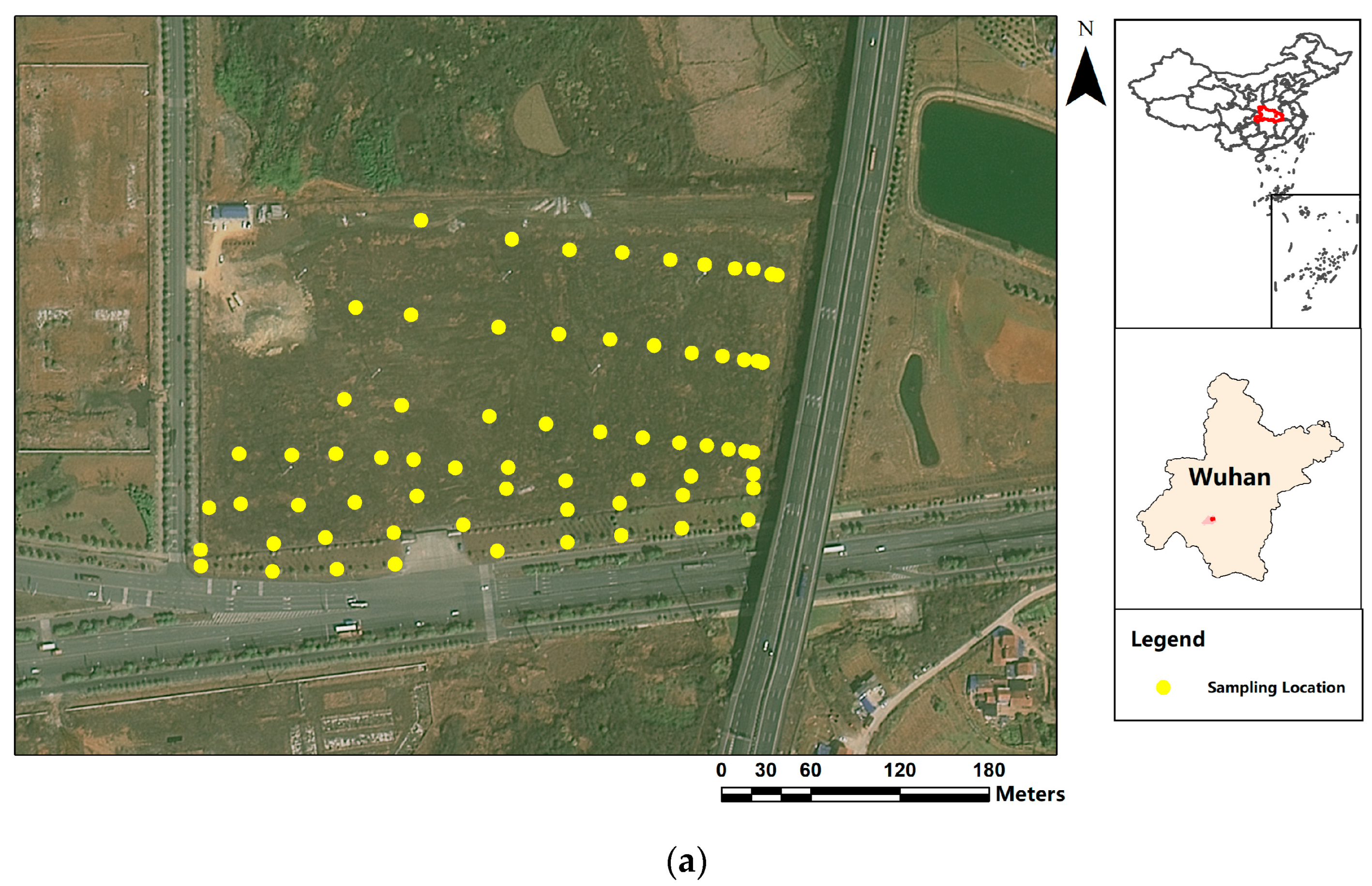
2.1. Study Area

The study area, with a total area of 0.113 km², is situated in the southern part of Wuhan City, China (Figure 1). It is bounded by Jin-Long Avenue West Line on the north and Wu-Shen Expressway on the east, extending until the junction of Jin-Long Avenue, Xue-Fu-Lan Avenue, and Kai-Di-La-Ke Road. The region is dominated by red, paddy, and yellow cinnamon soils, and the topography is flat. Two significant regional roads, Jin-Long Avenue and Xue-Fu-Lan Avenue, were constructed in 2015 and 2010, respectively, with substantial traffic flow posing a contamination threat to nearby areas. On the other hand, Kai-Di-La-Ke Road, an interior-connected road for the area, was erected in late 2019 with sparse traffic.

2.2. Materials

The study collected hyperspectral remote sensing data and soil samples on 20 December 2020, from 10:00 to 16:00, in the study area. During this time, the area was primarily characterized by shriveled seasonal grass and bare soil. The coordinates of the sampling points and the ground control points for the subsequent geometrical processing of the hyper-spectral images were recorded using a handheld global positioning system (GPS).

2.2.1. UAV Hyperspectral Remote Sensing Image Data Collection and Image Preprocessing

The hyperspectral remote sensing image data were captured using a DJI M600 Pro UAV equipped with a Cubert FireflEYE S185 hyperspectral imaging spectrometer (Bodkin Design & Engineering LLC, Newton, MA, USA), which has 125 spectral bands between 450 nm to 950 nm with a 4 nm spectral interval [32], which is shown in Figure 2. Images were acquired at a flight height of 115 m with a 5 cm ground spatial resolution. Before each flight, the hyperspectral sensor was radiometrically calibrated using a White Diffuse Reflectance Standard [33]. Multiple flights were carried out to cover the entire study area.

After the data acquisition, the UAV remote sensing data was preprocessed both geometrically and radiometrically as follows.

(a)

Geometric registration: Images from different flights were geometrically registered using the quadratic polynomial calculation model to eliminate the geometric distortions.

(b)

Radiometrical normalization: This process was used to eliminate the radiometrical inconsistency among the images acquired by different flights.

(c)

Image mosaic: The images acquired from different flights were mosaicked into a seamless wide-field image.

(d)

Geometric correction: The mosaicked image was geometrically corrected based on the ground control points.

All the geometric preprocessing was performed using ENVI software (Environment for Visualizing Images 5.3, L3Harris Geospatial Solutions, Inc, Broomfield, CO, USA). Radiometrical normalization was conducted using the global relative radiometrical normalization (RRN) method [34], which was implemented by Python.

2.2.2. On-Site Soil Data Collection and Processing

To ensure accurate soil data collection and processing, we considered the specific characteristics of the study area. A total of 72 soil samples were collected from 7 sampling lines that were parallel to Jin-Long Avenue (refer to Figure 1). Each soil sample weighed approximately 500 g and was collected from a soil layer depth of 0–20 cm. Within each sample plot, we collected soil samples from five different points, which were then combined [35]. One of the five points was located at the center of the plot, while the remaining four points were evenly distributed along the diagonal lines of the plot, ensuring equal spacing between the points.

The collected soil samples were air-dried at room temperature for three days. Subsequently, any residues of gravel, plant matter, and animal material were removed, and the soil samples were finely ground using an agate mortar. The ground soil samples were then sieved through a 100-mesh nylon sieve. The concentrations of heavy metals in the soil samples were measured at the test center of Wuhan Botanical Garden, Chinese Academy of Sciences [36,37]. The measurement process involved digesting 0.1 g of soil with a 4 mL mixed solution of 2:1 HNO3:HF (v/v) in a digestion tank. The samples underwent microwave digestion for 15 min, followed by dilution with deionized distilled water. Finally, the diluted solutions were analyzed using inductively coupled plasma atomic emission spectroscopy (ICP-OES Optima 8000dv, Perkin Elmer, Waltham, MA, USA).

After identifying each concentration, exploratory data analysis was carried out on the 72 samples, and 2 outliers were detected with the quartile–quartile method and removed.

3. Method

The methodology used in this study is summarized in Figure 3 and consists of four main parts: (1) preprocessing of UAV image data, (2) development of a retrieval model for predicting soil heavy metal concentrations, (3) retrieving of heavy metal concentrations in bare soil, and (4) analysis of heavy metal concentrations in the road-neighboring area.

3.1. Retrieval of Soil Heavy Metal Concentrations

3.1.1. Pretreatment of the Hyperspectral Data

The hyperspectral image was utilized to extract spectra from the soil sample points based on their spatial coordinates, using the data management tools available in ArcGIS software, version 10.7.1 (ESRI, Redlands, CA, USA). To enhance the spectral features and obtain more information about heavy metals in the soil, preprocessing of the original spectra data was conducted. Since the spectral response of soil heavy metal concentrations can be subtle and difficult to detect using conventional methods, a smoothing process was employed to reduce noise. The Savitzky–Golay (SG) filter, with an order of 2 and a frame size of 7 points (representing 28 nm), was applied for this purpose [15].

Following the smoothing process, four transformations were applied to the smoothed original reflectance: reciprocal, square root, exponential, and logarithmic. The logarithmic transformation was specifically used to enhance the differences in the visible region of wavelengths and reduce the impact of varying illumination conditions [38]. On the other hand, the reciprocal and exponential transformations were utilized to reduce the influence of noise by highlighting large spectral reflectance values and downplaying small ones [15,38]. Overall, these transformations aimed to mitigate the impact of background noise and the fluctuations in signal intensity resulting from spectral scattering and absorption on the soil surface.

In addition, Fractional Order Derivative (FOD) operations were performed to further highlight hidden information in the spectra. FODs have been used for the retrieval of soil HM concentrations and can identify the subtler spectral characteristics of heavy metals due to its gradual change in the treatment of the spectrum and is able to highlight hidden information [39]. We applied FODs with fractional orders ranging from 1.0 to 2.0, stepped by 0.2, resulting in six types of FODs for each spectrum.

All of the transformations were carried out using a self-developed Python program (Python 3.7) using the equation list in

Table 1. Spectral transformation.

Spectral Transformation	Formula
Reciprocal transformation	$R^{\prime }=1/R(\lambda )$
Logarithmic transformation	$R^{\prime }=Log(R(\lambda ))$
Square Root transformation	$R^{\prime }=Sqrt(R(\lambda ))$
Exponential transformation	$R^{\prime }=Exp(R(\lambda ))$

, and the FOD of $R(\lambda )$ is shown in Equation (1) [40], and $R(\lambda )$ is the reflectance of the band $\lambda$ of the hyperspectral remote sensing data.

To calculate FODs, in this study, we used the Grunwald–Letnikov (G-L) method, which is suitable for digital signal processing due to its simplicity and applicability to spectra [40]. The FOD of $R(\lambda )$ is based on the reflectance of two neighboring bands and given by Equation (1):

$$\frac{d^{v}R(\lambda )}{d{\lambda }^v}\approx R(\lambda )+(-v)R(\lambda -1)+\frac{(-v)(-v+1)}{2}f(\lambda -2)+\cdots +\frac{\Gamma (-v+1)}{n!\Gamma (-v+n+1)}f(\lambda -n)$$

(1)

where $v$ is the order of the differential, $R({\lambda }_{i+1})$ is the reflectance of band (“i + 1”), $R({\lambda }_{i-1})$ is the reflectance of band (“i − 1”), and $\Delta \lambda$ is the spectral interval of the bands. FOD computation for the 1-D signal is similar to the convolution process and is not applicable to the first band. Therefore, the FODs of the first band were not involved in the subsequent steps.

Finally, a total of 35 types of transformation were carried out over the 125 bands, resulting in 4375 spectral variates. All of these variates were used to identify the optimal spectral variables for soil heavy metal concentrations.

3.1.2. Optimal Spectral Variates Selection

In this study, a set of rules was used to select the optimal variates and avoid the situation of “dimensionality disaster”, which are significantly important and non-correlated spectral variates for retrieving concentrations of soil heavy metals Cr and Cu. The process involved the following steps.

Firstly, Spearman’s rank correlation coefficient [41,42] was calculated between the spectral variates and the concentrations of heavy metals. The spectral variates with a correlation at a significance level (p-value) of 0.01 were identified as candidate variates that were significantly correlated with the concentrations of heavy metals in soil.

Then, the Boruta algorithm was used for feature selection [43,44]. The Boruta algorithm is a variable selection method that iteratively removes features that are less significant than a random probe (artificial noise variables introduced by the Boruta algorithm).

Finally, to eliminate collinearity among the spectral variables and identify the optimal relevant spectral variables, the spectral variates determined by the Boruta algorithm were further checked. The correlation coefficient between the spectral variates was calculated, and the variates-pair with a correlation coefficient higher than 0.9 were analyzed, retaining only the one with the higher correlation coefficient with heavy metals concentrations.

3.1.3. Model Development and Selecting for Retrieving Soil HM Concentrations

This subsection outlines the development of models to extract heavy metal concentrations from remotely sensed data using selected spectral variables as independent variables, with heavy metal concentrations serving as the dependent variable. Before the development of a regression model, scatter plots were used to detect and eliminate outliers in the correlation between the heavy metals concentration and selected spectral variables.

(1)

The modeling methods.

Four regression techniques were employed to quantitatively retrieve soil Cr and Cu concentrations: multivariate linear regression (MLR), decision tree regression (DT), gradient-boosted decision tree regression (GBDT), and random forest regression (RF). DT, GBDT, and RF are commonly used data-driven machine learning methods [20,31].

    1.

Multivariate Linear Regressor (MLR)

MLR is the most basic form of regression analysis. It entails calculating the regression vector between an independent variable set (X) and a dependent variable. This method’s simplicity is its strongest advantage, particularly when weights are applied to the variables to minimize noise and enhance their significance. However, MLR has a significant disadvantage in that it presumes no collinearity between the variables, making proper selection of variables essential for accurate results.

    2.

Decision Tree Regressor (DT)

DT is a type of non-parametric, supervised learning method that is utilized for both classification and regression tasks [45]. The main goal of DT is to construct a model that can effectively predict the value of a target variable by learning simple decision rules derived from the features present in the data. The representation of a decision tree can be visualized as a stepwise approximation with constant values.

    3.

Gradient-Boosted Decision Trees Regressor (GBDT)

GBDT is a highly effective machine learning algorithm for fitting real-world data distributions, both for classification and regression problems [46]. It was developed by combining the decision tree algorithm with ensemble learning techniques such as bagging and boosting, addressing the overfitting problem that often arises in traditional decision tree algorithms. GBDT is known for its strong generalization ability and is widely used in many applications.

    4.

Random Forest Regressor (RF)

RF is a commonly employed algorithm for regression problems due to its high accuracy and simplicity [47,48]. It is an ensemble method that combines multiple decision trees using a voting mechanism. RF is typically trained using the bagging technique, which aggregates predictions from multiple models to enhance prediction accuracy compared to individual models. This algorithm exhibits robustness against outliers in the dataset and requires minimal parameter tuning.

(2)

Metrics for Evaluating Regression Models

Model accuracy was evaluated by comparing the predicted and measured concentrations of the testing set. Four parameters were used as indicators to evaluate model accuracy, namely the ${\mathrm{R}}^2$, root mean square error (RMSE), mean absolute error (MAE), and mean absolute relative error (MARE). Large ${\mathrm{R}}^2$ values and small RMSE values indicate higher model accuracy. The model with the highest accuracy for each heavy metal was selected for soil heavy metal content retrieval. Equations (2)–(5) were used to calculate ${\mathrm{R}}^2$, RMSE, MAE, and MARE:

$$R^2=1-\frac{{\displaystyle {\sum }_{i=1}^n{(y_i-{\widehat{y}}_i)}^2}}{{\displaystyle {\sum }_{i=1}^n{(y_i-{\overline{y}}_i)}^2}}$$

(2)

$$\mathrm{RMSE}=\sqrt{1/n{\sum }_{i=1}^n{(y_i-{\widehat{y}}_i)}^2}$$

(3)

$$MAE=\frac{1}{n{\displaystyle {\sum }_{i=1}^n\left|y_i-{\widehat{y}}_i\right|}}$$

(4)

$$MARE=\frac{1}{n{\displaystyle {\sum }_{i=1}^n\left|\frac{y_i-{\widehat{y}}_i}{{\widehat{y}}_i}\right|}}$$

(5)

where n represents the number of soil samples in the testing set, $y_i$ and ${\widehat{y}}_i$ represent the true value and predicted heavy metal content concentration of the ith soil sample in the testing set, respectively, and $\overline{y}$ is the average heavy metal concentration.

(3)

Model selection

The leave-one-out cross-validation (LOOCV) approach was employed to evaluate the performance of the models in predicting heavy metals. LOOCV is a type of cross-validation (CV) where one sample is excluded during each iteration. The average classification error obtained through LOOCV provides an unbiased estimate of the true error [49,50]. The dataset was divided into a training set and a testing set, where all but one observation were used for training the model, and the remaining sample was used for testing in each iteration. The constructed model was validated by comparing the predicted concentrations with the actual measured concentrations of the validation set, allowing for the evaluation of the model’s accuracy.

Grid search combined with repeated k-fold cross-validation was adopted for hyperparameter tuning to guarantee the best performance of each method [51]. Considering the size of the dataset, in the repeated k-fold cross-validation, the K and the repeated time were set as 3 and 7, respectively. Hyperparameters that generated the highest ${\mathrm{R}}^2$ were selected for model training.

The model with the highest ${\mathrm{R}}^2$ on the testing data was selected as the optimal model for predicting heavy metals subsequently. The retrieval models were established, utilizing the chosen regressor and the complete training dataset, and then implemented in all the bare soil regions to recover the HM concentrations.

All four models were developed using the Scikit-Learn machine-learning library in Python. All the processing and analysis were carried out using the self-developed Python program.

3.2. Analysis of Soil Heavy Metal Concentrations Characteristics

Various analytical processes were utilized to provide a comprehensive understanding of the soil heavy metal (HM) concentration characteristics within the studied region.

(1)

Correlation Analysis: Correlation analysis was conducted to reveal the inter-correlations among different HMs. A strong correlation may indicate that two types of heavy metals come from the same source [52,53]. In this study, the Pearson correlation coefficient was calculated to measure the degree of association between the concentrations of Cr and Cu in the soil samples [54].

(2)

Spatial Interpolation: Since only the HM concentrations over the bare soil pixels were retrieved, interpolation was employed to map the distribution of HM concentrations in the entire study area to provide a qualitative understanding of spatial trends and patterns, enabling visual interpretation and exploration of the data. The universal kriging (UK) interpolation tool in ArcGIS software (version 10.7.1, ESRI, Redlands, CA, USA) was used for this purpose. Kriging is a geostatistical interpolation method that considers both the distance and degree of variation between known data points when estimating values in unknown areas. UK, a kriging method with a local trend or drift, was used because it is appropriate for analyzing data with a specific trend [55].

(3)

Influence of Perpendicular Distance to the Road: The spatial distribution of HMs in the road-neighboring area is affected by various factors. In this study, the perpendicular distance of bare soil points from Jin-Long Avenue was calculated and analyzed as an external environmental factor. The relationship between this distance and soil HM concentrations was analyzed using the Data Management Tool in ArcMap 10.7 and a self-developed Python program.

4. Results and Discussion

4.1. Descriptive Statistics of Soil HMs Concentrations

The descriptive statistics of soil heavy metals (HMs) concentrations are presented in

Table 2. Statistics value for the measured soil heavy metal concentration in study area.

Heavy Metal		n 1	Min (mg/kg)	Max (mg/kg)	Mean (mg/kg)	Standard Deviation	C.V. 2 (%)	SBV 3	Pearson Correlation Coefficients
Cr	Total	70	68.034	133.843	104.987	11.091	10.564%	86.000	0.770 *
	<SBV	4	68.034	85.686	74.315	6.740	9.070%
	>SBV	66	88.975	133.843	105.539	11.314	10.720%
Cu	Total	70	24.952	41.109	33.920	3.349	9.879%	30.700
	<SBV	12	24.952	29.879	28.144	1.464	5.202%
	>SBV	58	30.918	41.109	34.729	2.688	7.740%

¹ Sample number. ² Coefficient of variation. ³ Background values of soil heavy metals in Hubei Province. * The correlation at a significance level (p-value) of 0.01.

, including the background values for Hubei Province [56]. The average contents of Cr and Cu were 104.987 mg/kg and 33.920 mg/kg, respectively. These values were higher than the recommended background values of 86 mg/kg and 30.7 mg/kg for Hubei Province. The background values for heavy metals are a critical indicator of soil environmental quality, reflecting the content of HMs in the soil environment that is not, or is less, influenced by human activities. The average concentrations of Cr and Cu were approximately 1.105 and 1.221 times higher than the background values suggested by Hubei Province, respectively. This implies that the heavy metals in the study region were caused by human activities. Additionally, the small coefficients of variation indicate that HM content remains reasonably constant throughout the study region. A strong positive correlation was observed between the concentrations of Cr and Cu in the soil, with Pearson correlation coefficients of 0.770 and a significance level (p-value) of 0.01. These results reveal a significant correlation between Cr and Cu and suggest that they may have originated from the same source.

4.2. Model Development and Selection for Heavy Metal Concentration Retrieval

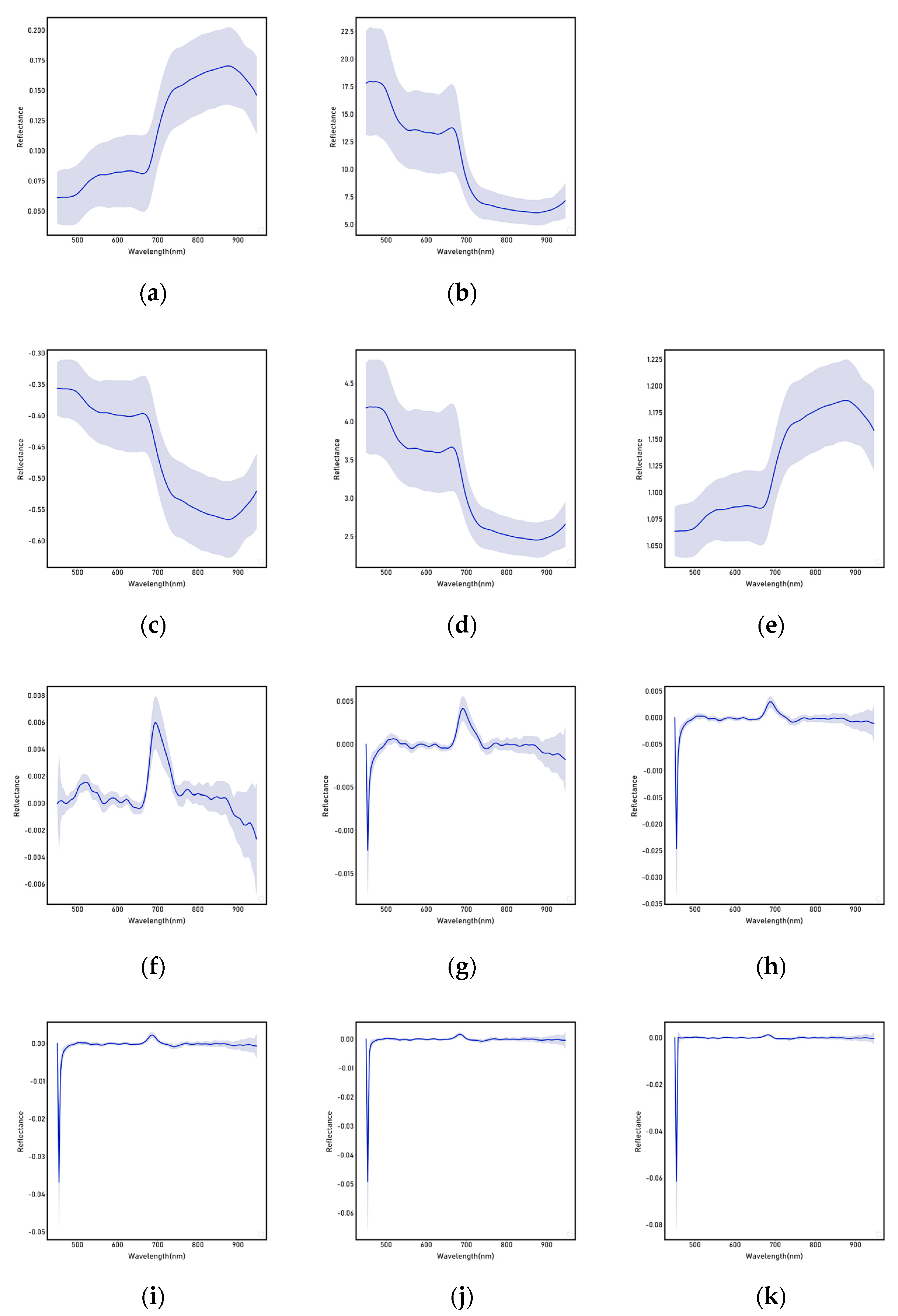
4.2.1. Spectral Transformations

Figure 4 presents the preprocessed reflectance data extracted from the hyperspectral image and its associated transformations. In total, 4375 spectral variables were obtained from 5 different types of spectrums (original reflectance and 4 spectral transformations) and 6 additional fractional differences of order (FODs) for each of them, covering 125 bands. Figure 4a–e show the smoothed original spectrums and four transformations, respectively, while Figure 4f–i demonstrate the FODs of the original reflectance. The original spectrums are relatively smooth, and the reflectance is similar to that of vegetation, which might be due to the mixture of vegetation and soil in the sampling sites. With an increase in fractional orders of FODs, the fractional differential values approach 0, indicating that the baseline drift and mixed overlapping peaks are gradually removed. All of these transformations and spectral indices were considered in identifying the best variables correlated with soil heavy metal content.

4.2.2. Selection of Optimal Spectral Variates

Spearman correlation coefficients with a significance level of 0.01 were utilized to determine the spectral variates that were significantly correlated with the heavy metal concentrations (Cr, Cu) in the soil. The correlation between the soil heavy metal concentrations (Cr, Cu) and all spectral variates is illustrated in Figure 5, which includes the smoothed original spectrum, four kinds of transformed spectrums, and their additional respective fractional order derivatives (FODs). The coefficients heatmap revealed that the spectral transformations could highlight the reflectance characteristics hidden in the soil spectral reflectance data compared to the original spectral variables. This was particularly evident for Cu, where only a few spectral variates had significant correlations in the original spectrum, but a large number of additional spectral variates with significant correlations with Cu concentrations were identified after transforming the original spectrum (Figure 5b). The spectral variates with a significant correlation (α = 0.01) were selected as candidate optimal variates. Through this variate sifting step, 846 and 441 variates were selected, respectively, for Cr and Cu.

The chosen spectral variables were analyzed using the Boruta algorithm to determine the optimal set of relevant variables for predicting the concentrations of soil’s heavy metals (Cr, Cu). The Boruta algorithm automatically categorized the spectral variables into three groups: unimportant, tentative, and important. The tentative and important groups were preserved, and the unimportant group of variates was ignored. Using this step, nine variates for Cr and eight variates for Cu were identified, respectively.

To address the sensitivity of regressors to collinearity among the independent variables, a correlation analysis was further performed to eliminate any collinearity among the spectral variables selected by the Boruta algorithm. Variate pairs with coefficients larger than 0.9 were checked, and the one with a smaller coefficient with HMs concentrations was removed. The final resulting optimal spectral variables for the two soil heavy metal concentrations and their correlation coefficients with HMs concentrations are listed in

Table 3. The optimal relevant spectral variates and the associated correlation coefficient for estimation concentrations of the two soil heavy metals.

Soil Heavy Metals	The Optimal Spectral Variables	Spearman Correlation Coefficient
Cr	Sqrt, FOD-1.2, 518 nm	0.433
	Exponential, 946 nm	0.405
	Reciprocal, FOD-1.0, 658 nm	−0.478
	Reciprocal, FOD-1.2, 742 nm	−0.427
	Reciprocal, FOD-1.4, 658 nm	−0.331
	Reciprocal, FOD-1.6, 710 nm	−0.514
Cu	Sqrt, FOD-1.8, 706 nm	−0.399
	Sqrt, FOD-2.0, 946 nm	−0.365
	Reciprocal, FOD-1.8, 510 nm	0.362
	Reciprocal, FOD-1.8, 666 nm	0.447
	Reciprocal, FOD-1.8, 702 nm	−0.421

, and the correlation coefficients between the selected spectral variables and the HMs could reach up to 0.514 for Cr and 0.447 for Cu. The correlation coefficient heatmap (Figure 6), which displays the correlation between the spectral variables, further illustrates that they exhibited relatively small correlations, indicating a limited presence of collinearity among the variates. The correlation coefficient heatmap (Figure 6) illustrates that the correlation between variates was small. It is noteworthy that the optimal variates for retrieving HMs concentrations were mainly from the FODs of the reciprocal transforming of the original spectrum, which is consistent with the study of Xu et al. [39].

4.2.3. Model Development and Selection for Heavy Metal Concentration Retrieval

The performance of the retrieval models for predicting the concentration of heavy metals (Cr and Cu) was assessed using the leave-one-out cross-validation (LOOCV) technique. The evaluation of the prediction performance involved comparing the predicted concentrations with the measured values using various metrics such as R², RMSE, MAE, and MARE. The results of the four models (RF, DT, MLR, and GBDT) for Cr and Cu are presented in

Table 4. Estimation model accuracy of Cr.

Parameter	Method		R2	MAE	RMSE	MARE
Cr	RF	Train	0.621	5.535	6.766	0.053
		Test	0.325	7.322	9.043	0.070
	Decision Tree	Train	0.338	7.242	8.930	0.069
		Test	0.252	7.925	9.516	0.076
	MLR	Train	0.397	7.011	8.546	0.067
		Test	0.264	7.738	9.442	0.074
	GBDT	Train	0.668	5.224	6.315	0.050
		Test	0.351	7.371	8.868	0.070

and

Table 5. Estimation model accuracy of Cu.

Parameter	Method		R2	MAE	RMSE	MARE
Cu	RF	Train	0.608	1.655	2.078	0.050
		Test	0.324	2.185	2.733	0.065
	Decision Tree	Train	0.311	2.237	2.752	0.067
		Test	0.116	2.479	3.124	0.074
	MLR	Train	0.380	2.139	2.615	0.064
		Test	0.246	2.377	2.886	0.071
	GBDT	Train	0.643	1.610	1.978	0.048
		Test	0.325	2.226	2.730	0.067

, respectively.

The four models performed differently when predicting heavy metal concentrations. RF and GBDT outperformed MLR and DT in predicting both Cr and Cu. GBDT had the highest R² values of 0.351 and 0.325 for Cr and Cu, respectively, indicating a moderate model fit [57,58,59]. RF closely followed with R² values of 0.324 and 0.325 for Cr and Cu, respectively. DT had the lowest R² values of 0.252 and 0.116 for Cr and Cu, respectively. Considering existing works [17,60] and factors such as vegetation interference, contamination levels in the study area, and the available spectral band range of the sensor, we deemed the model acceptable for subsequent work. As a result, GBDT was chosen to retrieve heavy metal content concentrations from bare soil points in the hyperspectral image. The scatter plots of the measured and predicted values for the four heavy metals using the optimal estimation models are presented in Figure 7.

4.3. The Spatial Character of the Soil HMs Concentrations

4.3.1. Spatial Distribution of HMs Concentrations

The spatial distribution map of the HMs concentrations was obtained using the universal kriging interpolation method based on the 17,420 bare soil points. After examining the semivariograms, we selected the exponential function as the kernel function for both Cu and Cr and applied kriging interpolation. This is displayed in Figure 8, which provides a visual representation of the concentration of the heavy metals across the study area and benefits understanding the spatial distribution patterns of the heavy metals in the study area.

The numerical analysis showed that the accumulation of Cr was generally higher than that of Cu compared to SBV. The spatial distribution of both Cu and Cr displayed high concentrations near roads and showed a declining trend from south to north, away from the road. No apparent association was observed between the distribution of soil heavy metals and the Wu-Shen Expressway. This could potentially be due to the height difference between the expressway and the study area, combined with the efficient drainage system, which effectively redirects pollutants to designated areas, reducing soil pollution in the study area.

The sources of heavy metal pollution in the road-adjacent soil are multifaceted, including traffic activities (such as gasoline exhaust, tire wear, and brake disc wear), the surrounding factories (such as fossil-fuel power stations and steelworks), and heavy metals naturally occurring in the soil parent material. However, no large-scale mining works or factories were found in the study area. Moreover, it is worth noting that the adsorption performance of Cu differs significantly from that of Cr in most soil types or soil components [61]. Hence, the spatial distribution pattern of heavy metals in this study area is unlikely to be the result of different pollution sources but rather is attributed to a similar source. In addition, the spatial heterogeneity of heavy metals from soil parent material is slight in small areas, further supporting the notion that road traffic activities are the primary source of heavy metal pollution in the area.

The spatial distribution of heavy metals is influenced by a multitude of factors, including the physical and chemical properties of the metals, wind direction, soil composition, and other environmental factors. Rainwater and air are common pathways for the spread of heavy metals from traffic. Meteorological statistical reports reveal that the frequency of north wind is higher than that of south wind in the study area [62], which could have hindered the southward diffusion of heavy metals adsorbed by particulate matter in the air. Given the relatively flat topography of the area, it is unlikely to have affected the spatial distribution of the HMs. The higher concentration of Cr compared to Cu may be attributed to a higher level of Cr pollution in the source or higher clay content in the soil, which has a higher adsorption capacity for Cr. Notably, the similarity in distribution pattern between Cr and Cu may be indicative of a shared source, as suggested by the correlation coefficient analysis in Section 4.1. However, the complex interplay between various environmental factors and the physical and chemical properties of heavy metals such as Cu and Cr makes it challenging, and further research is needed to definitively determine the underlying reasons behind the spatial distribution of these heavy metals.

4.3.2. Influence of the Perpendicular Distance to the Road

Figure 9 clearly shows a higher concentration of Cr and Cu near Jin-Long Avenue, with a gradual decrease in concentration as the perpendicular distance to the road increases. The relationship between soil HM concentrations and perpendicular road distance was analyzed using line charts, with perpendicular distance as the X-axis and heavy metal concentrations as the Y-axis. The results show that the concentration of Cr increased initially with increasing distance from the road edge before flattening out. Notably, the maximum concentration was not observed at the road edge. On the other hand, the concentration of Cu showed a continuous decrease with increasing perpendicular distance from the road.

Typically, Cu and Cr ions adhere to different particles, which can cause them to migrate and diffuse differently through the soil after being transported by rain or air. The size of the particles carrying HMs can also affect their settlement location. For instance, heavy metals contained in smaller particles may precipitate closer to the road, while larger particles may settle further away. The intricate nature of the mechanisms leading to the spatial distribution of HMs in the soil is further complicated by external factors such as prevailing wind direction and vehicle speed, which can affect air turbulence on the road and further influence the settling location of HMs. In our analysis, the higher concentration of Cr compared to Cu may be due to a higher level of Cr pollution in the source, or the higher clay content in the soil, which has a higher adsorption capacity for Cr. Our findings indicate that soil heavy metals (Cr and Cu) are generated by traffic-related activities and show their spatial distribution pattern, but the exact mechanism remains unclear. Further research, incorporating the study of aerodynamics and soil environmental chemistry, may be required to fully understand the characteristics of heavy metal distribution in this area.

5. Conclusions

In conclusion, this study aimed to develop and apply HM retrieval models using UAV-based hyperspectral image samples to analyze the spatial distribution and accumulation characteristics of heavy metals (HMs) in road-adjacent soil. We successfully built HM retrieval models by selecting optimal spectral variates through correlation analysis and the Boruta algorithm. Four regression models, including MLR, DT, RF, and GBDT, were developed and compared using the LOOCV procedure, with GBDT demonstrating the best performance for both HM concentrations.

By applying the HM retrieval model to bare soil points identified through supervised classification, we generated a spatial interpolation map of HM concentrations in the soil using the universal kriging interpolation method. Our findings revealed that the concentrations of the two heavy metals, Cu and Cr, were significantly enriched at the edges of the road, gradually decreasing with increasing perpendicular distance from the road. This study effectively explored the fine-scale distribution of soil HM concentrations and provided insights into the accumulation character in specific areas of interest.

However, this study does have some limitations that warrant improvement in future research. The relatively small number of samples used to develop the estimation models may have affected the accuracy and robustness of the retrieval models. Future studies should focus on collecting a larger number of soil samples to enhance model performance. Additionally, the R-square values on the test data were not as high as those based on laboratory-measured spectra or for areas with high HM concentrations. Factors such as vegetation interference, contamination levels, and the choice of spectral bands used for HM detection (Vis-NIR in this study) may have influenced the accuracy of our work. Future studies should address these factors and carefully consider instrumental stability and radiometric and geometric preprocessing of hyperspectral images to minimize biases.

Furthermore, in terms of understanding the mechanisms underlying the spatial distribution of Cu and Cr in soil, this study primarily presented the distribution of HM concentrations and briefly inferred some possible reasons. Further research is required to fully comprehend these mechanisms, including the analysis of particulate content in road dust, prevailing wind direction, vehicle speed, and other relevant factors. Meanwhile the reliability of geospatial interpolation is of utmost importance to facilitate in-depth exploration and analysis.

Overall, it is crucial to comprehensively understand the patterns of HM pollution to effectively mitigate environmental and human health risks. Therefore, further research in this field is needed to develop a more comprehensive understanding of the complex mechanisms involved.

References

1. Shi, T.; Guo, L.; Chen, Y.; Wang, W.; Shi, Z.; Li, Q.; Wu, G. Proximal and Remote Sensing Techniques for Mapping of Soil Contamination with Heavy Metals. Appl. Spectrosc. Rev. 2018, 53, 783–805. [Google Scholar] [CrossRef]
2. Yang, Z.; Zhang, R.; Li, H.; Zhao, X.; Liu, X. Heavy Metal Pollution and Soil Quality Assessment under Different Land Uses in the Red Soil Region, Southern China. Int. J. Environ. Res. Public Health 2022, 19, 4125. [Google Scholar] [CrossRef]
3. Ma, T.; Zhang, Y.; Hu, Q.; Han, M.; Li, X.; Zhang, Y.; Li, Z.; Shi, R. Accumulation Characteristics and Pollution Evaluation of Soil Heavy Metals in Different Land Use Types: Study on the Whole Region of Tianjin. Int. J. Environ. Res. Public Health 2022, 19, 10013. [Google Scholar] [CrossRef]
4. Sert, E.B.; Turkmen, M.; Cetin, M. Heavy Metal Accumulation in Rosemary Leaves and Stems Exposed to Traffic-Related Pollution near Adana-İskenderun Highway (Hatay, Turkey). Environ Monit Assess 2019, 191, 553. [Google Scholar] [CrossRef]
5. Hamzeh, M.A.; Aftabi, A.; Mirzaee, M. Assessing Geochemical Influence of Traffic and Other Vehicle-Related Activities on Heavy Metal Contamination in Urban Soils of Kerman City, Using a GIS-Based Approach. Environ Geochem Health 2011, 33, 577–594. [Google Scholar] [CrossRef]
6. Khalifa, A.A.; Darwish, M. Estimation of Lead Concentration in Settled Dust at Gharian City, Libya. MAYFEB J. Environ. Sci. 2017, 1, 6–10. [Google Scholar]
7. Heidari, M.; Darijani, T.; Alipour, V. Heavy Metal Pollution of Road Dust in a City and Its Highly Polluted Suburb; Quantitative Source Apportionment and Source-Specific Ecological and Health Risk Assessment. Chemosphere 2021, 273, 129656. [Google Scholar] [CrossRef]
8. Wang, G.; Zeng, C.; Zhang, F.; Zhang, Y.; Scott, C.A.; Yan, X. Traffic-Related Trace Elements in Soils along Six Highway Segments on the Tibetan Plateau: Influence Factors and Spatial Variation—ScienceDirect. Sci. Total Environ. 2017, 581–582, 811–821. [Google Scholar] [CrossRef]
9. Nikolaeva, O.; Rozanova, M.; Karpukhin, M. Distribution of Traffic-Related Contaminants in Urban Topsoils across a Highway in Moscow. J. Soils Sediments 2017, 17, 1045–1053. [Google Scholar] [CrossRef]
10. She, W.; Guo, L.; Gao, J.; Zhang, C.; Wu, S.; Jiao, Y.; Zhu, G. Spatial Distribution of Soil Heavy Metals and Associated Environmental Risks near Major Roads in Southern Tibet, China. Int. J. Environ. Res. Public Health 2022, 19, 8380. [Google Scholar] [CrossRef]
11. Sutherland, R.A. Lead in Grain Size Fractions of Road-Deposited Sediment. Environ. Pollut. 2003, 121, 229–237. [Google Scholar] [CrossRef] [PubMed]
12. Hua, M.; Zhu, B.W.; Liao, Q.L.; Pan, Y.M.; Yang, J.; Feng, J.S. Preliminary Research on Pollution Level of Heavy Metals in Farmland Soils along Both Sides of Main Roads in Jiangsu. J. Geol. 2008, 32, 165–171. [Google Scholar]
13. Yan, X.; Gao, D.; Zhang, F.; Zeng, C.; Xiang, W.; Zhang, M. Relationships between Heavy Metal Concentrations in Roadside Topsoil and Distance to Road Edge Based on Field Observations in the Qinghai-Tibet Plateau, China. Int. J. Environ. Res. Public Health 2013, 10, 762–775. [Google Scholar] [CrossRef] [Green Version]
14. Enuneku, A.; Biose, E.; Ezemonye, L. Levels, Distribution, Characterization and Ecological Risk Assessment of Heavy Metals in Road Side Soils and Earthworms from Urban High Traffic Areas in Benin Metropolis, Southern Nigeria. J. Environ. Chem. Eng. 2017, 5, 2773–2781. [Google Scholar] [CrossRef]
15. Liu, Z.; Lu, Y.; Peng, Y.; Zhao, L.; Hu, Y. Estimation of Soil Heavy Metal Content Using Hyperspectral Data. Remote. Sens. 2019, 11, 1464. [Google Scholar] [CrossRef] [Green Version]
16. Kumar, V.; Sharma, A.; Kaur, P.; Singh Sidhu, G.P.; Bali, A.S.; Bhardwaj, R.; Thukral, A.K.; Cerda, A. Pollution Assessment of Heavy Metals in Soils of India and Ecological Risk Assessment: A State-of-the-Art. Chemosphere 2019, 216, 449–462. [Google Scholar] [CrossRef] [PubMed]
17. Wang, F.; Gao, J.; Zha, Y. Hyperspectral Sensing of Heavy Metals in Soil and Vegetation: Feasibility and Challenges. ISPRS J. Photogramm. Remote. Sens. 2018, 136, 73–84. [Google Scholar] [CrossRef]
18. Mulder, V.L.; de Bruin, S.; Schaepman, M.E.; Mayr, T.R. The Use of Remote Sensing in Soil and Terrain Mapping—A Review. Geoderma 2011, 162, 1–19. [Google Scholar] [CrossRef]
19. Gan, W.; Xu, J.; Feng, S.; Xiaodi, H.U.; Anna, X.; Suxun, S. Spatial Statistical Characteristics of the Heavy Metal Pollution at the Road Side Soil-A Case in Jiang-Xia District of Wuhan. J. Geomat. 2022, 47, 49–53. [Google Scholar]
20. Mouazen, A.M.; Nyarko, F.; Qaswar, M.; Tóth, G.; Gobin, A.; Moshou, D. Spatiotemporal Prediction and Mapping of Heavy Metals at Regional Scale Using Regression Methods and Landsat 7. Remote. Sens. 2021, 13, 4615. [Google Scholar] [CrossRef]
21. Chen, H.W.; Chen, C.-Y.; Nguyen, K.L.P.; Chen, B.-J.; Tsai, C.-H. Hyperspectral Sensing of Heavy Metals in Soil by Integrating AI and UAV Technology. Environ. Monit. Assess. 2022, 194, 518. [Google Scholar] [CrossRef]
22. Wei, L.; Zhang, Y.; Lu, Q.; Yuan, Z.; Li, H.; Huang, Q. Estimating the Spatial Distribution of Soil Total Arsenic in the Suspected Contaminated Area Using UAV-Borne Hyperspectral Imagery and Deep Learning. Ecol. Indic. 2021, 133, 108384. [Google Scholar] [CrossRef]
23. Zhang, Y.; Wei, L.; Lu, Q.; Zhong, Y.; Yuan, Z.; Wang, Z.; Li, Z.; Yang, Y. Mapping Soil Available Copper Content in the Mine Tailings Pond with Combined Simulated Annealing Deep Neural Network and UAV Hyperspectral Images. Environ. Pollut. 2023, 320, 120962. [Google Scholar] [CrossRef] [PubMed]
24. Tang, J.; Alelyani, S.; Liu, H. Feature Selection for Classification: A Review. In Data Classification: Algorithms and Applications; CRC Press: Boca Raton, FL, USA, 2014. [Google Scholar]
25. Kemper, T.; Sommer, S. Estimate of Heavy Metal Contamination in Soils after a Mining Accident Using Reflectance Spectroscopy. Environ. Sci. Technol. 2002, 36, 2742. [Google Scholar] [CrossRef]
26. Kokaly, R.F.; Clark, R.N. Spectroscopic Determination of Leaf Biochemistry Using Band-Depth Analysis of Absorption Features and Stepwise Multiple Linear Regression. Remote. Sens. Environ. 1999, 67, 267–287. [Google Scholar] [CrossRef]
27. Wu, Y.; Chen, J.; Wu, X.; Tian, Q.; Ji, J.; Qin, Z. Possibilities of Reflectance Spectroscopy for the Assessment of Contaminant Elements in Suburban Soils. Appl. Geochem. 2005, 20, 1051–1059. [Google Scholar] [CrossRef]
28. Mi, L. Based on the Spectral Variation of Vegetation Monitoring the Heavy Metal Pollution of Soil. Earth Sci. Front. 2009, 3, 17. [Google Scholar]
29. Nagaraju, T.V.; Mantena, S.; Azab, M.; Alisha, S.S.; El Hachem, C.; Adamu, M.; Rama Murthy, P.S. Prediction of High Strength Ternary Blended Concrete Containing Different Silica Proportions Using Machine Learning Approaches. Results Eng. 2023, 17, 100973. [Google Scholar] [CrossRef]
30. Taghizadeh-Mehrjardi, R.; Fathizad, H.; Ali Hakimzadeh Ardakani, M.; Sodaiezadeh, H.; Kerry, R.; Heung, B.; Scholten, T. Spatio-Temporal Analysis of Heavy Metals in Arid Soils at the Catchment Scale Using Digital Soil Assessment and a Random Forest Model. Remote. Sens. 2021, 13, 1698. [Google Scholar] [CrossRef]
31. Fang, Y.; Xu, L.; Wong, A.; Clausi, D.A. Multi-Temporal Landsat-8 Images for Retrieval and Broad Scale Mapping of Soil Copper Concentration Using Empirical Models. Remote. Sens. 2022, 14, 2311. [Google Scholar] [CrossRef]
32. Copyright 2021 Cubert GmbH. Available online: https://www.cubert-hyperspectral.com/Products/Firefleye-185 (accessed on 15 September 2022).
33. UAV Calibration Board: Radiation Calibration and Reflectance Calibration. Available online: https://www.gzchanghui.com/product_view_37_163.html (accessed on 18 May 2023).
34. Gan, W.; Shen, H.; Zhang, L.; Gong, W. Normalization of Medium-Resolution NDVI by the Use of Coarser Reference Data: Method and Evaluation. Int. J. Remote. Sens. 2014, 35, 7400–7429. [Google Scholar] [CrossRef]
35. Jin, X.; Li, Z.; Yang, G.; Yang, H.; Feng, H.; Xu, X.; Wang, J.; Li, X.; Luo, J. Winter Wheat Yield Estimation Based on Multi-Source Medium Resolution Optical and Radar Imaging Data and the AquaCrop Model Using the Particle Swarm Optimization Algorithm. ISPRS J. Photogramm. Remote. Sens. 2017, 126, 24–37. [Google Scholar] [CrossRef]
36. Wu, Y.; Chen, J.; Ji, J.; Gong, P.; Liao, Q.; Tian, Q.; Ma, H. A Mechanism Study of Reflectance Spectroscopy for Investigating Heavy Metals in Soils. Soil. Sci. Soc. Am. J. 2007, 71, 918–926. [Google Scholar] [CrossRef]
37. Public Laboratory Platform. Available online: http://www.wbg.cas.cn/Gglabplat/Index.Html. (accessed on 15 September 2022).
38. Lei, W.; You-lu, B.A.; Yan-li, L.U.; He, W.A. Effect on Retrieval Precision for Corn N Content by Spectrum Data. Remote. Sens. Technol. Appl. 2011, 26, 220–225. [Google Scholar]
39. Xu, X.; Chen, S.; Ren, L.; Han, C.; Lv, D.; Zhang, Y.; Ai, F. Estimation of Heavy Metals in Agricultural Soils Using Vis-Nir Spectroscopy with Fractional-Order Derivative and Generalized Regression Neural Network. Remote. Sens. 2021, 13, 2718. [Google Scholar] [CrossRef]
40. Wang, X.; Zhang, F.; Kung, H.T.; Johnson, V.C. New Methods for Improving the Remote Sensing Estimation of Soil Organic Matter Content (SOMC) in the Ebinur Lake Wetland National Nature Reserve (ELWNNR) in Northwest China. Remote. Sens. Environ. 2018, 218, 104–118. [Google Scholar] [CrossRef]
41. Xiao, C.; Ye, J.; Esteves, R.M.; Rong, C. Using Spearman’s Correlation Coefficients for Exploratory Data Analysis on Big Dataset. In Concurrency and Computation: Practice and Experience; John Wiley and Sons Ltd.: Hoboken, NJ, USA, 2016; Volume 28, pp. 3866–3878. [Google Scholar]
42. Sedgwick, P. Spearman’s Rank Correlation Coefficient. BMJ 2014, 349, g7327. [Google Scholar] [CrossRef] [Green Version]
43. Kursa, M.B.; Rudnicki, W.R. Feature Selection with the Boruta Package. J. Stat. Softw. 2010, 36, 1–13. [Google Scholar] [CrossRef] [Green Version]
44. Rudnicki, W.R.; Wrzesień, M.; Paja, W. All Relevant Feature Selection Methods and Applications. Stud. Comput. Intell. 2015, 584, 11–28. [Google Scholar] [CrossRef]
45. Breiman, L.; Friedman, J.H.; Olshen, R.A.; Stone, C.J. Classification and Regression Trees, 1st ed.; Chapman & Hall/CRC: Boca Raton, FL, USA, 1984. [Google Scholar]
46. Song, Y.; Niu, R.; Xu, S.; Ye, R.; Peng, L.; Guo, T.; Li, S.; Chen, T. Landslide Susceptibility Mapping Based on Weighted Gradient Boosting Decision Tree in Wanzhou Section of the Three Gorges Reservoir Area (China). ISPRS Int. J. Geoinf. 2019, 8, 4. [Google Scholar] [CrossRef] [Green Version]
47. Ho, K. The Random Subspace Method for Constructing Decision Forests. IEEE Trans. Pattern Anal. Mach. Intell. 1998, 20, 832–844. [Google Scholar]
48. Breiman, L. Random Forests. Mach. Learn. 2001, 45, 5–32. [Google Scholar] [CrossRef] [Green Version]
49. Kohavi, R. A Study of Cross-Validation and Bootstrap for Accuracy Estimation and Model Selection. In Proceedings of the International Joint Conference on Artificial Intelligence, Montreal, QC, Canada, 20–25 August 1995. [Google Scholar]
50. Varma, S.; Simon, R. Bias in Error Estimation When Using Cross-Validation for Model Selection. BMC Bioinform. 2006, 7, 91. [Google Scholar] [CrossRef] [Green Version]
51. Bergstra, J.; Bengio, Y. Random Search for Hyper-Parameter Optimization. J. Mach. Learn. Res. 2012, 13, 281–305. [Google Scholar]
52. Zhang, J.; Hua, P.; Krebs, P. Influences of Land Use and Antecedent Dry-Weather Period on Pollution Level and Ecological Risk of Heavy Metals in Road-Deposited Sediment. Environ. Pollut. 2017, 228, 158. [Google Scholar] [CrossRef]
53. Benesty, J.; Chen, J.; Huang, Y. On the Importance of the Pearson Correlation Coefficient in Noise Reduction. IEEE Trans. Audio Speech Lang. Process. 2008, 16, 757–765. [Google Scholar] [CrossRef]
54. Borjac, J.; El Joumaa, M.; Kawach, R.; Youssef, L.; Blake, D.A. Heavy Metals and Organic Compounds Contamination in Leachates Collected from Deir Kanoun Ras El Ain Dump and Its Adjacent Canal in South Lebanon. Heliyon 2019, 5, e02212. [Google Scholar] [CrossRef] [Green Version]
55. ArcMap. Available online: https://www.esri.com/zh-cn/arcgis/products/arcgis-desktop/resources (accessed on 15 September 2022).
56. China Environmental Monitoring Station. Chinese Soil Element Background Value; China Environmental Science Press: Beijing, China, 1990. [Google Scholar]
57. Hair, J.; Black, W.; Babin, B.; Anderson, R. Multivarite Data Analysis, 7th ed.; Prentice Hall: Englewood Cliffs, NJ, USA, 2010. [Google Scholar]
58. Neter, J.; Kutner, H.; Nachtsheim, C. Applied Linear Statistical Models; McGraw-Hill/Irwin: New York, NY, USA, 1996; Volume 4. [Google Scholar]
59. Cohen, J. Statistical Power Analysis for the Behavioral Sciences, 2nd ed.; Academic Press: Cambridge, MA, USA, 1988. [Google Scholar]
60. Shi, T.; Chen, Y.; Liu, Y.; Wu, G. Visible and Near-Infrared Reflectance Spectroscopy—An Alternative for Monitoring Soil Contamination by Heavy Metals. J. Hazard. Mater. 2014, 265, 166–176. [Google Scholar] [CrossRef]
61. Li, Q.; Wang, Y.; Li, Y.; Li, L.; Tang, M.; Hu, W.; Chen, L.; Ai, S. Speciation of Heavy Metals in Soils and Their Immobilization at Micro-Scale Interfaces among Diverse Soil Components. Sci. Total Environ. 2022, 825, 153862. [Google Scholar] [CrossRef]
62. China Meteorological Science Data Sharing Service Network. Available online: https://www.cdc.cma.gov.cn (accessed on 15 September 2022).
Figure 1. The location of the study area and the sample points (marked as yellow circles). (a) The general study area based on the China’s GaoJing satellite image. (b) The specific study area using the observed Hyperspectral image.
Sustainability 15 10043 g001aSustainability 15 10043 g001b
Figure 2. UAV-based hyperspectral observation platform and the white diffuse reflectance standard.
Sustainability 15 10043 g002
Figure 3. Flow chart of the proposed method.
Sustainability 15 10043 g003
Figure 4. The original hyperspectral data and the four transformations (a) original reflectance, (b) square root, (c) reciprocal, (d) exponential transformation, and (e) logarithmic. The reflectance processed by fraction-order derivative (take original reflectance as example) in (f) 1.0−order, (g) 1.2−order, (h) 1.4−order, (i) 1.6−order, (j) 1.8−order, (k) 2.0−order. The dark blue line represents the mean value of the spectrum, and the light blue areas represent the standard deviations.
Sustainability 15 10043 g004
Figure 5. The absolute Spearman correlation coefficients matrix of hyperspectral reflectance data and 4375 (5 × 7 × 125) spectral variates for (a) Cr, (b) Cu (p = 0.01). The x-axis represents the wavelengths and the y-axis represents the transformations and their corresponding first order derivatives (FODs). The y-axis consists of 5 parts from top to bottom, including the original reflectance, square root, logarithms, exponential, and reciprocal transforming of the original reflectance, and each of the parts contains the spectrum and its corresponding FODs with orders from 1.0 to 2.0. The correlation coefficients for the insignificant variates (p-value = 0.01) were set to 0.0 and denoted by deep purple.
Sustainability 15 10043 g005
Figure 6. Correlation matrix for the optimal spectral variates. (a) Variates for Cr, (b) variates for Cu.
Sustainability 15 10043 g006
Figure 7. Scatterplots of predicted and measured soil heavy metals using the GBDT model. (a) Soil Cu concentrations and (b) soil Cr concentrations.
Sustainability 15 10043 g007
Figure 8. The spatial distribution of the soil heavy metal concentration of (a) Cu and (b) Cr respectively.
Sustainability 15 10043 g008
Figure 9. Variation of heavy metal concentrations with distance away from the Jin-Long Avenue for (a) Cr and (b) Cu respectively.
Sustainability 15 10043 g009