TMR-Array-Based Pipeline Location Method and Its Realization

Abstract

Pipeline inspection is important to ensure the safe operation of pipelines. Obtaining the location of an underground pipeline is a prerequisite for most inspection technologies. Existing pipeline location methods can find a pipeline’s location, but they require multiple measurements and cannot be used by automatic inspection robots. In this paper, a tunnel magnetoresistance (TMR)-sensor-array-based pipeline location method is proposed to solve this problem. Firstly, a detection probe is designed using a TMR sensor array. It is calibrated by the improved ellipsoid fitting method to measure the magnetic field around the pipeline accurately. Secondly, a relative pipeline-position-locating method is proposed by detecting the phases of the magnetic induction signals at different frequencies. Thirdly, a three-dimensional pipeline location method is proposed. The horizontal and vertical distances and the angle between the pipeline and the probe are calculated by measuring the magnetic induction amplitude. Finally, a simulation model and a test platform are established, and the experimental results illustrate that, by adopting the TMR array, the three-dimensional pipeline location method can locate a pipeline in real time in three dimensions with good accuracy.

1. Introduction

As a continuous long-distance transportation method, pipeline transport has long occupied a dominant position in the transportation of oil, natural gas, and other liquid and gas forms of energy [1,2,3]. However, when pipelines have been in service for decades, their surface anti-corrosion coating and metal materials deteriorate or even become damaged [4,5,6], which seriously affects the safety of pipeline operations and can even lead to leakages [7,8], resulting in substantial economic losses and environmental hazards. In order to improve the reliability of pipeline transport, pipelines need to be inspected periodically. The inspection interval is generally 3 to 5 years [9,10], and the calculation of a pipeline’s position is one of the necessary steps in pipeline inspection.

The commonly used pipeline inspection methods can be classified as discontinuous methods, software-based methods, and hardware-based continuous methods. Among these methods, discontinuous and software-based inspection methods are mainly adopted for surface pipelines or pipelines with leakages; they have substantial application limitations [11,12]. Therefore, the most typical detection method is to detect the abnormal areas of the pipeline through various external hardware sensors, such as magnetic and acoustic sensors [13]. Pipeline inspection systems and the principles behind them have been continuously developed and improved in recent decades.

In terms of detecting the magnetic signals of pipelines, Bell Laboratories proposed a dual-antenna pipeline detector, which used differential signals from two horizontal coils to locate pipelines and could detect the depth of pipelines when directly above them [14]. Li Ruixi et al. combined the pipeline current mapper (PCM) pipeline exploration instrument with the total station to improve the measurement accuracy, thus measuring the buried depth of pipelines with an error of ±0.15 m above the pipeline [15]. Cui Dandan et al. improved the magnetic gradient method in wells. By digging a vertical shaft with a depth of two meters, the magnetic gradient transformation generated by pipeline currents could be analyzed, and a formula for estimating a pipeline’s buried depth and horizontal position was obtained [16]. Yizhen Zhao et al. proposed a target signal extraction algorithm to ascertain the locations of parallel steel pipelines and recognize defects based on TMR sensors, which is of great significance for the application of non-destructive testing (NDT) in pipeline in-line inspection [17]. The uncertainties in pipeline inspections and estimations of the size and probability of corrosion defects should be considered for the management of the health of pipelines. Julio et al. summarized the methods adopted in the estimation of a pipeline’s remaining life [18,19]. The reliability of corroded pipelines is usually assessed by probabilistic tools that consider the uncertainties associated with the size of any corrosion defects.

The pipeline inspection methods above are limited by the insufficient precision of the coil used to detect the magnetic field. It is difficult to measure the magnetic induction intensity around the pipeline accurately. This method thus cannot realize the precise three-dimensional location of the pipeline. Measuring the exact depth of a pipeline requires the probe to be directly above the pipeline, which limits the application of this technique significantly.

In terms of accurately locating pipelines, Fang Xingguo et al. adopted an ENVI magnetometer and calculated the buried depth of pipelines through the ratio circle intersection method according to the magnetic field theory of infinite horizontal cylinders and achieved good results [20]. Wang Hongzhi et al. adopted a multi-sensor fusion scheme, a dual-frequency side-scan sonar, a high-resolution submarine profiler, and a magnetometer, and, through the use of these tools combined with underwater robot technology, realized the high-precision location of deep-sea pipelines and the detection of surface sediment on pipelines [21]. The BPS river-crossing pipeline detection system of Canada’s BPS Company and the one-pass river crossing pipeline detection system of America’s STARTRAK company adopted magnetic detection technology and combined it with underwater sonar technology to realize the detection of the general position of underwater pipelines at large buried depths and to generate a sectional map of the pipelines’ locations [22,23].

The pipeline inspection methods above used additional means to assist the inspection in order to locate the accurate three-dimensional position of the pipeline, which increased the cost of pipeline inspection. It is difficult to popularize these methods over an extensive range, and it is also important to note that they cannot be integrated into robots [24] or applied to automatic non-destructive pipeline inspection methods, which have been widely adopted for decades [25].

In order to solve the problems above and locate the accurate three-dimensional positions of buried pipelines in a timely fashion and at lower costs, we propose a tunnel magnetoresistance (TMR)-array-based pipeline locating method. In this paper, the detection probe is redesigned using a TMR array, which is laid out vertically to the ground to detect the three-dimensional component of magnetic induction intensity. In order to improve the accuracy of the location process, an improved ellipsoid fitting method is proposed to calibrate the TMR sensors. Finally, a method to locate the accurate three-dimensional position is proposed according to the redesigned probe structure, which is verified by simulations and experiments. The technological processes are shown in Figure 1.

The main contributions of this paper are summarized as follows:

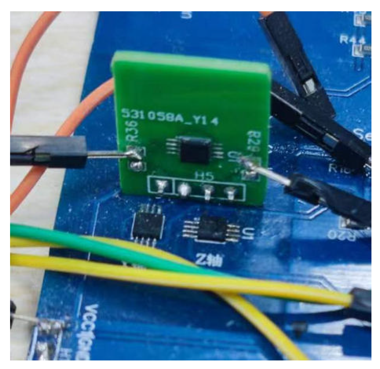
• The detection probe is redesigned to locate pipelines accurately. By adopting TMR sensors as linear magnetic sensors, magnetic fields surrounding pipelines can be detected accurately, and the difficulties of traditional PCM receiving equipment are conquered.
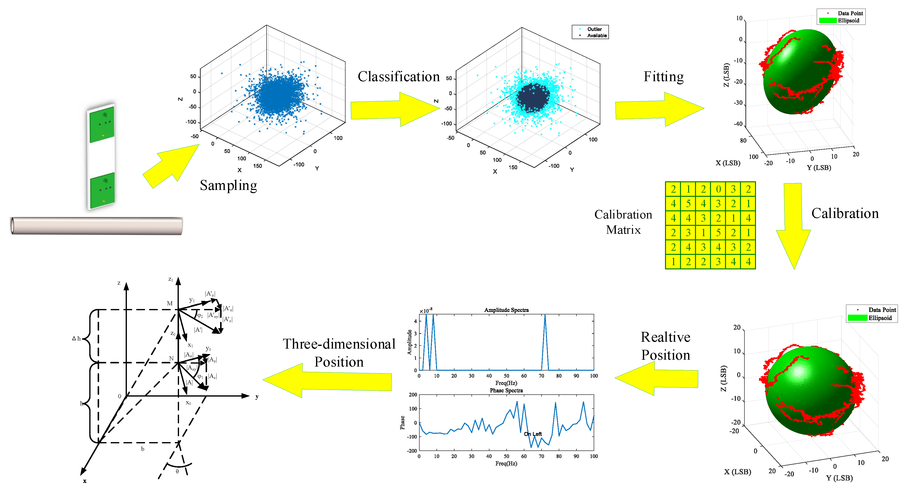
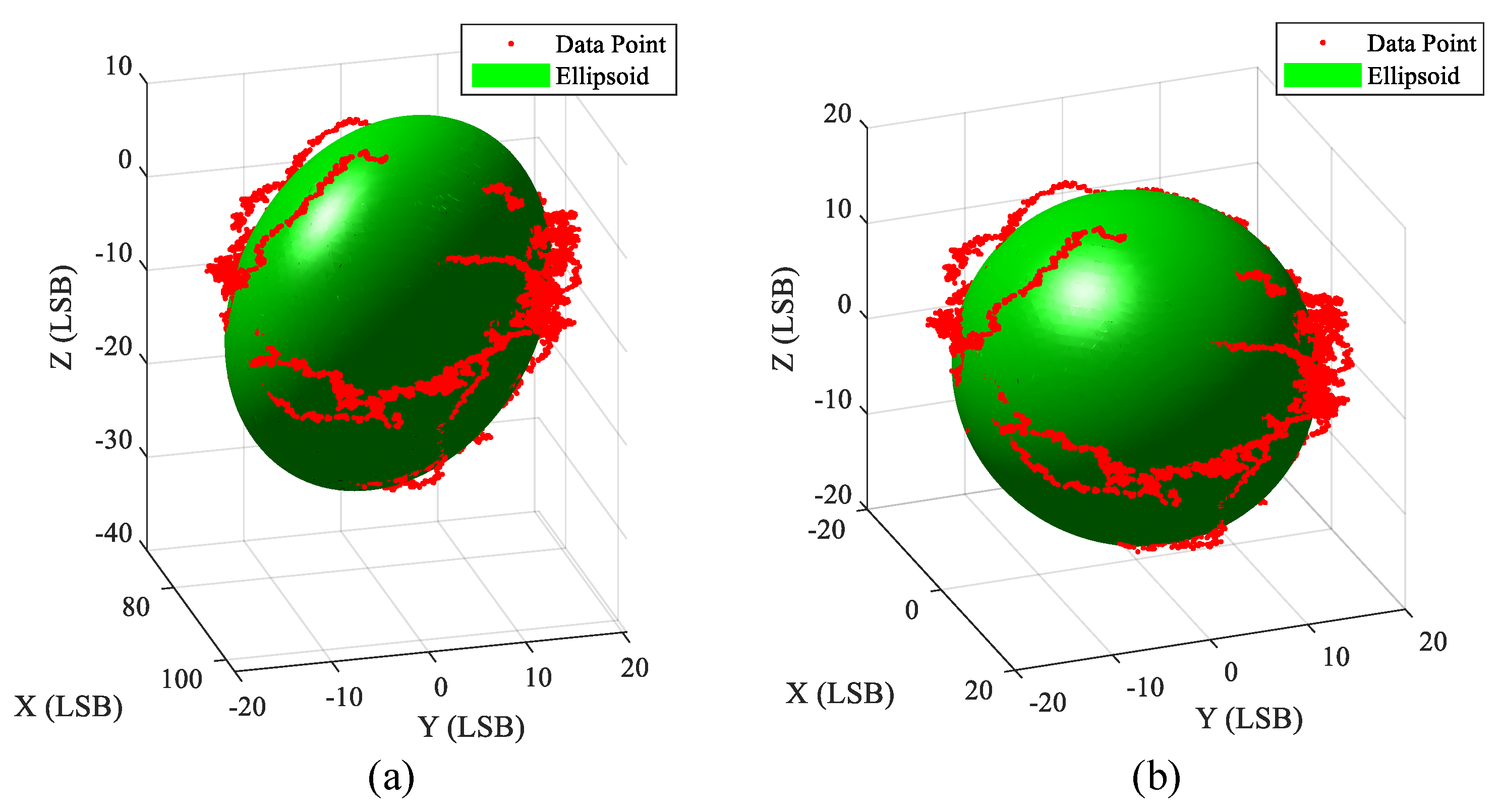
• An improved ellipsoid fitting method is proposed to calibrate the TMR array. The Gaussian mixture model (GMM) binary classification method is adopted to eliminate the invalid data collected by the TMR array and generated by the ADC jitter. The ellipsoid fitting method is adopted to calibrate the TMR array and acquire data without invalidations. It improves the calibration effect, eliminates non-orthogonal and sensitivity errors, and improves accuracy when detecting magnetic induction intensity.
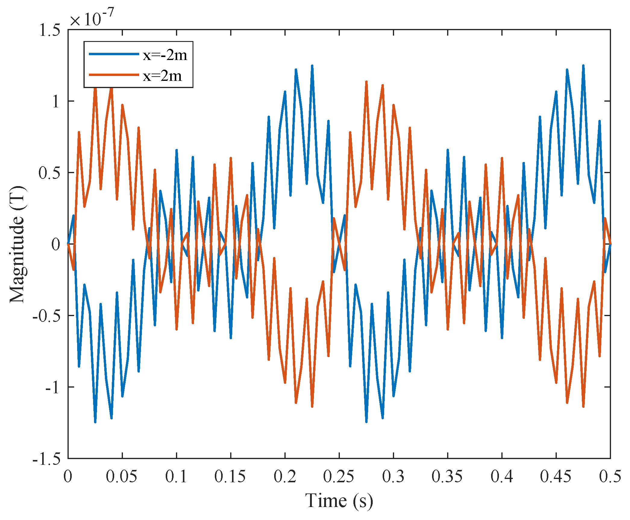
• A relative pipeline position location method is proposed. Based on the relationships of the lag times of different frequency signals generated around pipelines, this method is adopted to locate the detection probe’s left or right side relative to the pipeline. Compared with the PCM, which locates the pipeline by the amplitude of signals from different detection coils, our method improves the reliability of position detection.
• A three-dimensional pipeline location method is proposed. Based on the relationships of the amplitudes of the three-dimensional components of the magnetic induction intensity in different directions and positions around the pipeline, this method is proposed to calculate the three-dimensional position of pipelines, including the horizontal angle, vertical distance, and horizontal distance between the sensor and the pipeline, respectively. Compared with the PCM, which can only locate the rough direction of the pipeline, our method improves the accuracy and efficiency of the location process.
• A TMR array calibration experiment and three-dimensional location experiment are conducted to evaluate the proposed methods. The experimental results illustrate that the three-dimensional pipeline location method adopting the redesigned detection probe can locate the pipeline in three dimensions with satisfactory linearity and a low average error.

The rest of this paper is organized as follows. Section 2 introduces the principle of PCM. Section 3 introduces the proposed method. Section 4 carries out the simulations and the experiments, and their results are also discussed. Section 5 concludes this article.

2. The Principle of PCM

In this section, the principle of the PCM for pipeline location is introduced, and problems relevant to the process of locating piplelines in three-dimensional space are analyzed.

As shown in Figure 2a, in the detection process, a high-power signal transmitter, which has one terminal connected to the pipeline test pile and the other terminal grounded, generates the current signal with a specific frequency and emits it into the pipeline. Pipeline inspection personnel hold the PCM receiving equipment to detect the magnetic field generated by the underground pipeline and record the pipeline’s location [26,27,28]. A PCM, which is a practical device, is shown in Figure 2b.

The probe structure adopted by the PCM detection method comprises eight coils, as shown in Figure 3. The embedded microprocessor detects the signals of the coils, and the position of the pipeline relative to the probe can be located by the relationship between the signal intensities, as shown in

Table 1. Probe signal intensity and pipe position relationship.

Signal Intensity	Pipeline Position
$U_2>U_3$, $U_4=U_5$	Left
$U_2>U_3$, $U_4>U_5$	Front left
$U_2=U_3$, $U_4>U_5$	Front
$U_2<U_3$, $U_4>U_5$	Front right
$U_2<U_3$, $U_4=U_5$	Right
$U_2<U_3$, $U_4<U_5$	Rear right
$U_2=U_3$, $U_4<U_5$	Rear
$U_2>U_3$, $U_4<U_5$	Rear left

, where $U_1$–$U_8$ represent the signal intensities of the coils in Figure 3.

When locating a pipeline’s depth, the personnel need to roughly locate the position of the pipeline according to Table 1. The personnel walking to the area near the pipeline can calculate the buried depth of the pipeline according to Equation (1) [29],

$$h=\frac{d_1{U}_8}{U_1-U_8}$$

(1)

where $d_1$ represents the vertical distance between Coil 1 and Coil 8.

As can be seen, the PCM method cannot locate the pipeline continuously or accurately but can only locate the rough direction of the pipeline. Moreover, the depth of the pipeline can be located only when the probe is directly above it. Therefore, the application of PCM has significant limitations. To improve the accuracy of pipeline detection, we adopt TMR sensors, rather than coils, to detect the magnetic signals precisely in real time. Additionally, the method of pipeline detection proposed in this paper is based on the PCM method, which emits a current with specific frequencies into the pipeline to generate an electromagnetic signal to locate the pipeline in three dimensions.

3. Materials and Methods

We propose a theoretical model to locate a pipeline’s accurate three-dimensional position. The main contents of this section are as follows:

• The error sources of the TMR array are analyzed, the calibration model of the sensors is established, and the accurate measurement of the magnetic induction intensity is realized.
• A relative pipeline position location method is proposed to detect whether the pipeline is positioned left or right relative to the detection probe.
• A three-dimensional pipeline location method is proposed to ocate the three-dimensional position of pipelines.

3.1. Calibration of TMR Array

Three single-axis TMR magnetic sensors are adopted and used as a set to constitute three-axis magnetic sensors as magnetic detection devices in this paper. In actual measurement applications, magnetic sensors operating in three directions have performance differences from each other [30,31]. The errors inherent to these sensors can be described as non-orthogonal, sensitivity, and zero-bias errors [32]. The definition of non-orthogonal error is shown in Figure 4. The influence of non-orthogonal, sensitivity, and zero-bias errors on measurement results are shown in Equations (2)–(4), respectively.

$$\left(\begin{array}{c}{X}_v\\ Y_v\\ Z_v\end{array}\right)={\mathit{C}}_v\left(\begin{array}{c}{X}_0\\ Y_0\\ Z_0\end{array}\right)=\left(\begin{array}{ccc}cos\varphi cos\phi & cos\varphi sin\phi & sin\varphi \\ 0& cos\psi & sin\psi \\ 0& 0& 1\end{array}\right)\left(\begin{array}{c}{X}_0\\ Y_0\\ Z_0\end{array}\right)$$

(2)

where $X_v$, $Y_v$, and $Z_v$ represent the measured values of the TMR array after considering the sensitivity error. ${\mathit{C}}_v$ represents the sensitivity error matrix. $X_0$, $Y_0$, and $Z_0$ represent the measured value of the three-axis magnetic sensor under ideal conditions.

$$\left(\begin{array}{c}{X}_s\\ Y_s\\ Z_{\mathrm{s}}\end{array}\right)={\mathit{C}}_s\left(\begin{array}{c}{X}_0\\ Y_0\\ Z_0\end{array}\right)=\left(\begin{array}{ccc}{k}_1& 0& 0\\ 0& k_2& 0\\ 0& 0& k_3\end{array}\right)\left(\begin{array}{c}{X}_0\\ Y_0\\ Z_0\end{array}\right)$$

(3)

where $X_s$, $Y_s$, and $Z_s$ represent the measured values of the TMR array after considering the non-orthogonal error. ${\mathit{C}}_s$ represents the non-orthogonal error matrix.

$$\left(\begin{array}{c}{X}_b\\ Y_b\\ Z_b\end{array}\right)=\left(\begin{array}{c}{X}_0\\ Y_0\\ Z_0\end{array}\right)+\mathit{b}$$

(4)

where $X_b$, $Y_b$, and $Z_b$ represent the measured values of the TMR array after considering the zero-bias error. ${\mathit{C}}_b$ represents the zero-bias error matrix. $\mathit{b}$ represents the zero-bias vector.

Considering the errors above, the error model of the TMR array can be represented by Equation (5),

$${\mathit{H}}_r=\left(\begin{array}{c}{X}_r\\ Y_r\\ Z_r\end{array}\right)={\mathit{C}}_s{\mathit{C}}_v\left(\begin{array}{c}{X}_0\\ Y_0\\ Z_0\end{array}\right)+\mathit{b}=\mathit{C}{\mathit{H}}_0+\mathit{b}$$

(5)

where ${\mathit{H}}_r$ represents the measured value vector and ${\mathit{H}}_0$ represents the measured value vector under ideal conditions. ${\mathit{C}}_b$ represents the error matrix.

The ellipsoid fitting method is adopted to calibrate the TMR array [33]. To achieve this, we rotate the TMR array in space, collect the output signal of the sensors, and fit it into an ellipsoid, as shown in Equations (6) and (7).

$$\begin{array}{c}{\mathit{H}}_0={\left({\mathit{C}}_s{\mathit{C}}_v\right)}^{-1}({\mathit{H}}_r-\mathit{b})\hfill \\ \to {\mathit{H}}_0={\left(\begin{array}{ccc}cos\varphi cos\phi & cos\varphi sin\phi & sin\varphi \\ 0& cos\psi & sin\psi \\ 0& 0& 1\end{array}\right)}^{-1}{\left(\begin{array}{ccc}{k}_1& 0& 0\\ 0& k_2& 0\\ 0& 0& k_3\end{array}\right)}^{-1}({\mathit{H}}_r-\mathit{b})\hfill \end{array}$$

(6)

$$a{H_x}^2+b{H_y}^2+c{H_z}^2+2f{H}_x{H}_y+2g{H}_x{H}_z+2h{H}_y{H}_z+2p{H}_x+2q{H}_y+2r{H}_z-1=0$$

(7)

where $H_x$, $H_y$, and $H_z$ represent the measured values of the TMR array.

The elements in Equation (6), which turn out to be Equation (8), are adopted to calibrate the TMR array.

$$\left\{\begin{array}{c}{\mathrm{k}}_x=\sqrt{a^{\prime }}\hfill \\ {\mathrm{k}}_y=\sqrt{b^{\prime }}\hfill \\ k_z=\sqrt{c^{\prime }}\hfill \\ \varphi =arcsin(\frac{e^{\prime }}{\sqrt{a^{\prime }{c}^{\prime }}})\hfill \\ \phi =arcsin(\frac{d^{\prime }{c}^{\prime }-e^{\prime }{f}^{\prime }}{\sqrt{(a^{\prime }{c}^{\prime }-e{}^{\prime 2})(b^{\prime }{c}^{\prime }-f{}^{\prime 2})}})\hfill \\ \psi =arcsin(\frac{f^{\prime }}{\sqrt{b^{\prime }{c}^{\prime }}})\hfill \end{array}\right.$$

(8)

3.2. Pipeline Location and Calculation Model

In this section, the relative pipeline position location method and the three-dimensional pipeline location method are proposed.

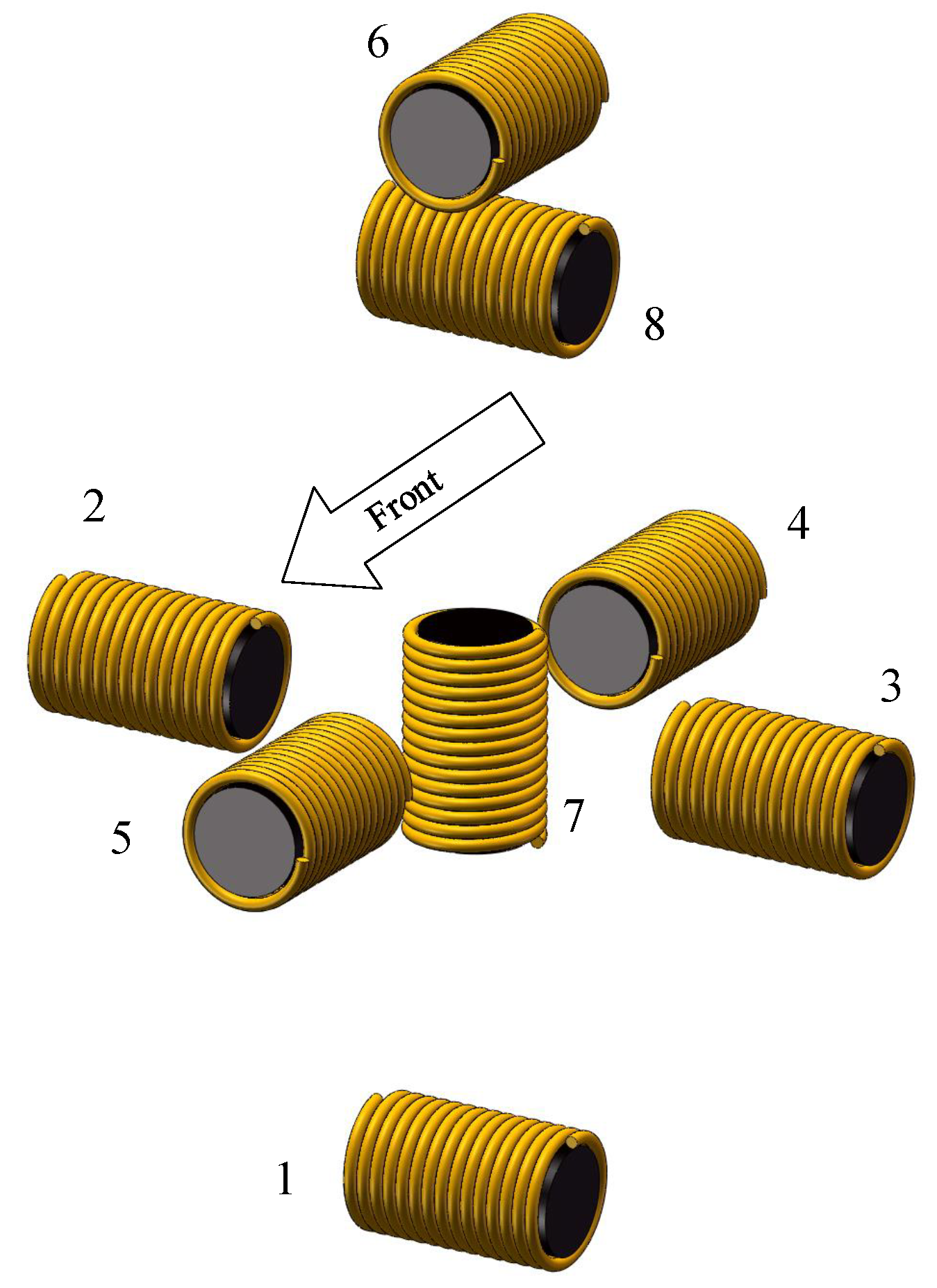
3.2.1. Redesigned Detection Probe

The problem with traditional probes, which use coils, is that they cannot measure the magnetic field and locate the position of a pipeline accurately. In order to conquer the difficulty above, a new probe model is proposed in this section.

As shown in Figure 5, the detection probe consists of two printed circuit boards (PCBs) and a support structure. Each PCB consists of a set of linear magnetic sensors perpendicular to each other, a set of signal-amplifying circuits, and a set of signal–output interfaces.

When the detection probe moves around the pipeline, the magnetic sensors detect the magnetic field generated by the pipeline and convert it into a differential voltage signal. The signal-processing circuit converts the differential signal into a single-ended signal and amplifies it for long-distance transmission. Finally, the signal is transmitted to the signal processing circuit through the signal–output interface using shielded wires.

The amplitude of the magnetic signal generated by the pipeline is vulnerable. The selection of appropriate magnetic-sensitive devices is necessary to improve the magnetic signal’s reliability, considering that the TMR sensor has apparent advantages in resolution, linearity, sensitivity. and other performance indicators. Each TMR sensor detects magnetic induction intensity components in one direction, which can significantly improve the accuracy of magnetic signal detection.

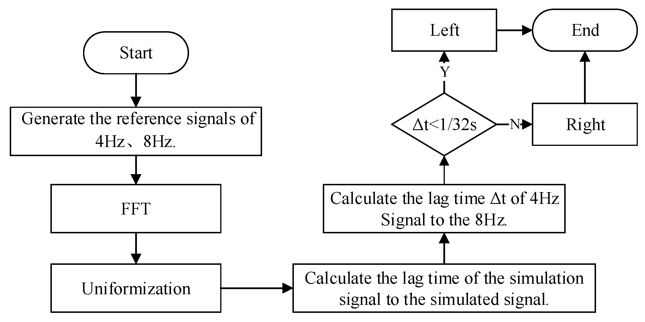
3.2.2. Relative Pipeline Position Location Method

Our relative pipeline position location method is proposed to calculate the phase difference in the signal detected by the detection probe to determine whether the probe is positioned left or right relative to the pipeline. The processes are as follows:

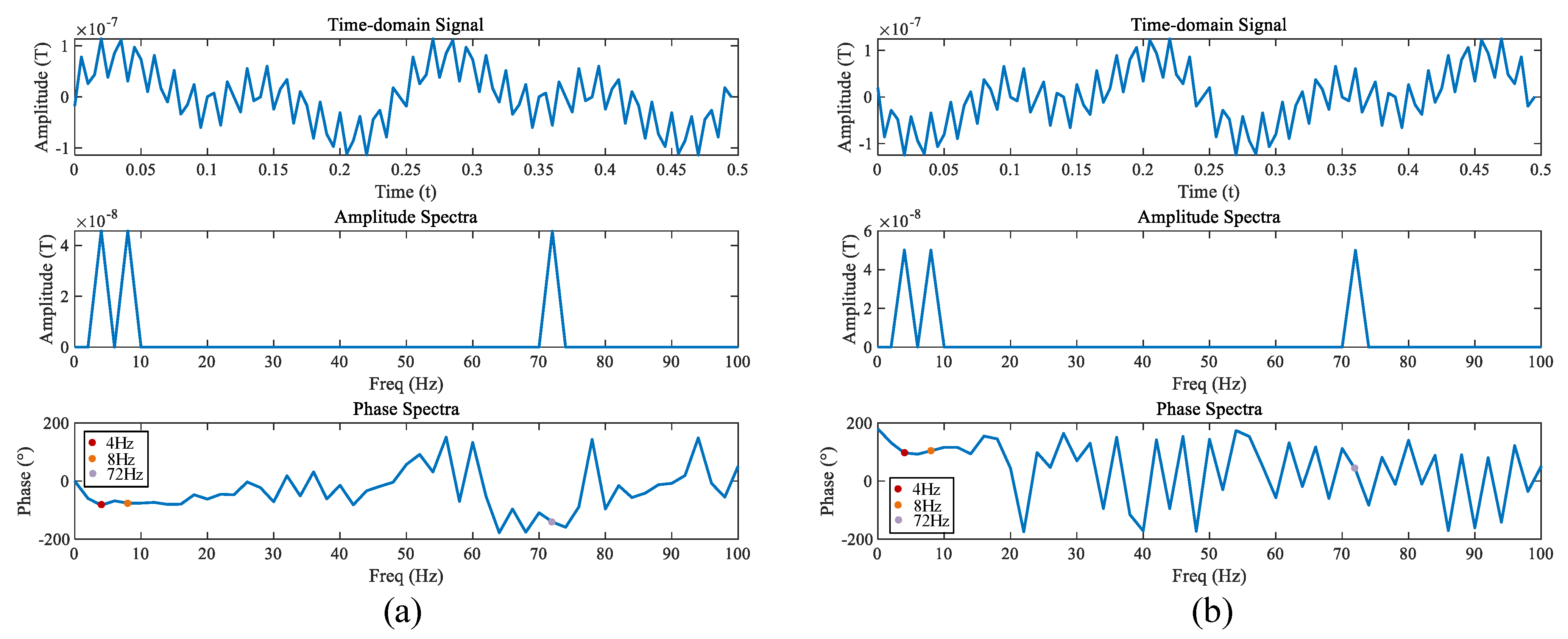
• Transform the signal by FFT and extract the phase and amplitude information. The amplitudes $|X_y\left[4\right]|$ and $|X_y\left[8\right]|$ and phase angles ${\omega }_{y4Hz}$ and ${\omega }_{y8Hz}$ are obtained for 4 Hz and 8 Hz signals, respectively, along the Y-axis.
• Supposing that data are obtained on the left side of the pipeline, the lag time $\Delta t_{y4Hz}$ of the signal’s phase at the detected location ${\omega }_{y4Hz}$ relative to the probe at the emitted position ${\omega }_{y04Hz}$ can be represented by Equation (9),

  $$\Delta t_{y4Hz}=\frac{{\omega }_{y4Hz}-{\omega }_{y04Hz}}{8\pi }$$

  (9)
• The lag time $\Delta t_{y8Hz}$ of the signal’s phase at the detected location ${\omega }_{y8Hz}$ relative to the probe at the emitted position ${\omega }_{y08Hz}$ can be represented by Equation (10),

  $$\Delta t_{y8Hz}=\frac{{\omega }_{y8Hz}-{\omega }_{y08Hz}}{16\pi }$$

  (10)
• The time difference $\Delta t$ between $\Delta t_{y4Hz}$ and $\Delta t_{y8Hz}$ is expressed in Equation (11),

  $$\Delta t=\Delta t_{y4Hz}-\Delta t_{y8Hz}=\frac{2{\omega }_{y4Hz}-{\omega }_{y8Hz}-(2{\omega }_{y04Hz}-{\omega }_{y08Hz})}{16\pi }$$

  (11)
• The phases of the 4 Hz and 8 Hz signals $\omega {}_{y4Hz}^{\prime }$ and $\omega {}_{y8Hz}^{\prime }$ on the right side are, respectively, expressed by Equation (12) and Equation (13),

  $${\omega }_{y4Hz}^{\prime }={\omega }_{y4Hz}+\pi$$

  (12)

  and

  $${\omega }_{y8Hz}^{\prime }={\omega }_{y8Hz}+\pi$$

  (13)
• The lag time $\Delta t_{y8Hz}^{\prime }$ of the signal’s phase at the detected location ${\omega }_{y8Hz}^{\prime }$ relative to the probe at the emitted position ${\omega }_{y08Hz}^{\prime }$ can be represented by Equation (14),

  $$\begin{array}{c}\Delta t^{\prime }=\frac{2{\omega }_{4Hz} - {\omega }_{8Hz} + \pi - (2{\omega }_{y04Hz} - {\omega }_{y08Hz})}{16\pi }\hfill \end{array}$$

  (14)
• Since the phases of the 4 Hz and 8 Hz are the same at the position of signal emission, the current lag times of the 4 Hz and 8 Hz signals are the same for transmissions over identical distances. This can be expressed as $\Delta t_{y8Hz}=\Delta t_{y4Hz}$, as shown in Equation (15),

  $$\begin{array}{c}{\omega }_{y8Hz}=2{\omega }_{y4Hz}\hfill \end{array}$$

  (15)
• The lag times of the 4 Hz and 8 Hz signal compared to the reference signal are the same, as shown in Equation (16).

  $${\omega }_{y08Hz}=2{\omega }_{y04Hz}$$

  (16)
• By susbtituting Equations (15) and (16) into Equations (11) and (14), we obtain $\Delta t=0$ and $\Delta t^{\prime }=1/16$, respectively.
• The position of the pipeline relative to the probe can be located. The threshold $\Delta t=1/32$ is assigned. When $\Delta t<1/32$, the probe is on the left side of the pipeline. Otherwise, the probe is on the right side of the pipeline.

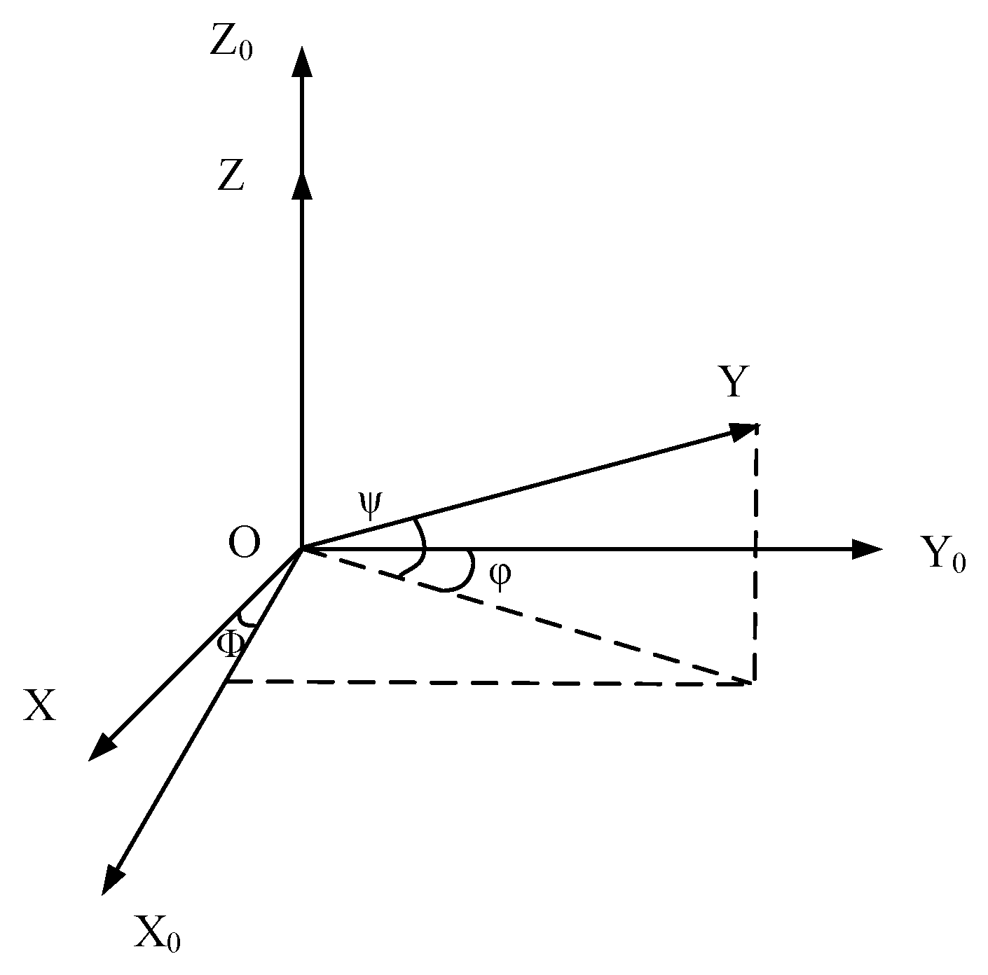
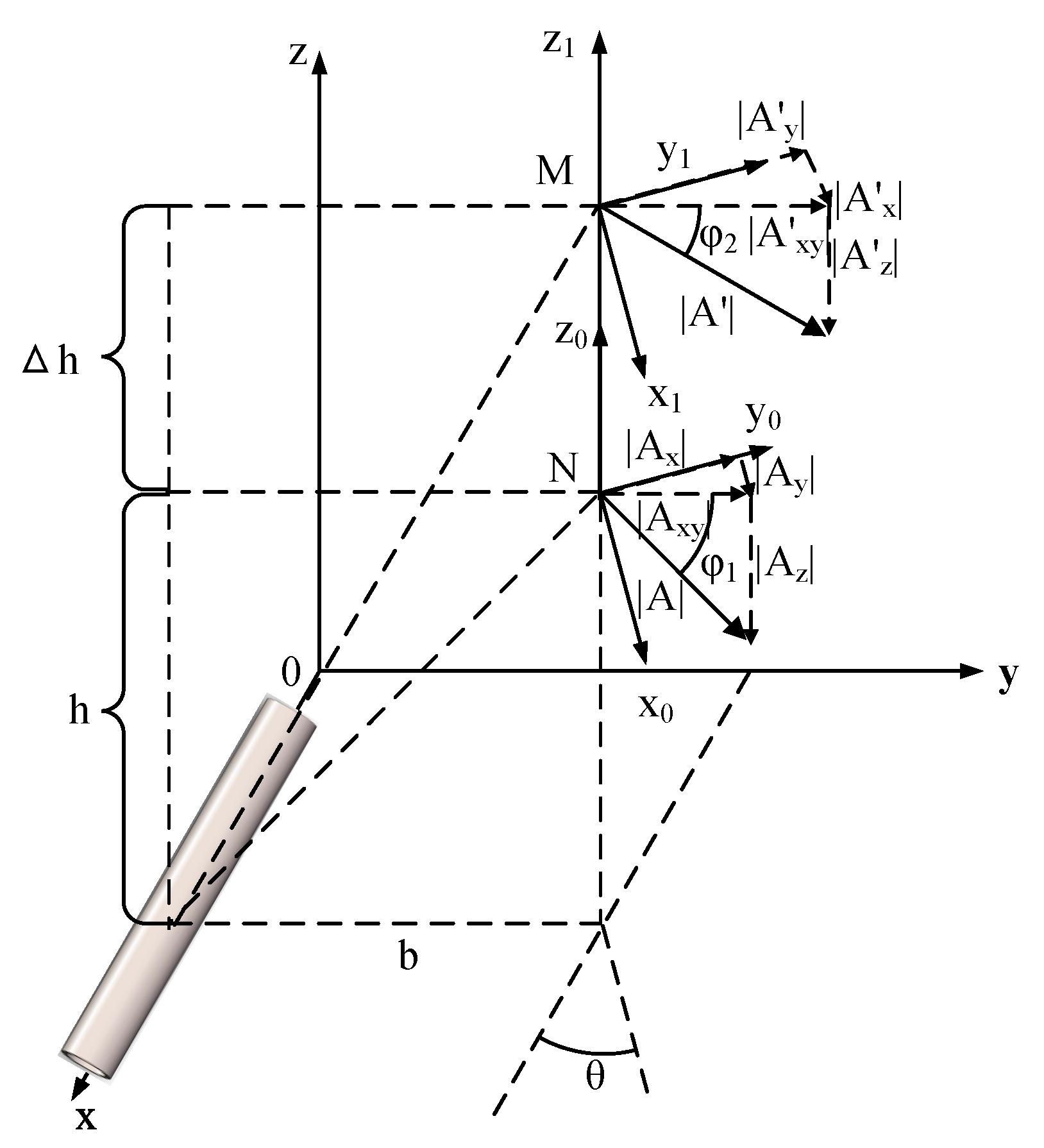
3.2.3. Three-Dimensional Pipeline Location Method

A three-dimensional pipeline location method is proposed in this section that allows us to locate the position of a pipeline accurately, including the horizontal angle, vertical distance, and horizontal distance between the detection probe and the pipeline. Two sets of TMR arrays are utilized to calculate the magnetic induction intensity in different directions. The pipeline is assumed to coincide with the X-axis, as shown in Figure 6.

We assign the intermediate variables according to Equations (17) and (18),

$$m=\frac{h}{b}=\frac{|A_{xy}|}{|A_z|}=\frac{\sqrt{|A_x{|}^2+|A_y{|}^2}}{|A_z|}$$

(17)

$$n=\frac{h+\Delta h}{b}=\frac{|A{}_{xy}^{\prime }|}{|A{}_z^{\prime }|}=\frac{\sqrt{|A{}_x^{\prime }{|}^2+|A{}_y^{\prime }{|}^2}}{|A{}_z^{\prime }|}=\frac{\Delta h}{b}+m$$

(18)

The three-dimensional pipeline position can be obtained by Equations (19)–(21).

$$b=\frac{\Delta h}{n-m}$$

(19)

$$h=\frac{m\Delta h}{n-m}$$

(20)

$$\theta =arctan\left(\frac{|A_x|}{|A_{\mathrm{y}}|}\right)$$

(21)

Through the upper and bottom sensors, the three-dimensional components of the magnetic induction intensity are measured and substituted into Equations (17), (18) and (21). The horizontal and vertical distance between the detection probe and the pipeline can be calculated by substituting m and n into Equations (19) and (20). The horizontal angle between the positive direction of the detection probe and the pipeline can be calculated by substituting a value into Equation (21).

4. Results and Discussion

In this section, according to the theoretical model above, the correctness of the calibration of the three-axis magnetic sensor, the relative pipeline position location method, and the three-dimensional pipeline location method are verified from simulations and experiments.

4.1. Calibration Experiment of Three-Axis TMR Array

In order to improve the accuracy of three-axis magnetic field detection and pipeline positioning, the single-axis TMR magnetic sensor TMR2705 was adopted as the magnetic sensor, as shown in Figure 7. In the figure, the unit is the least significant bit (LSB), which represents the magnetic intensity converted by the ADC. Each unit of LSB represents $8.06\times {10}^{-3}$ Gauss.

During the calibration process, the ADC sample values randomly jitter and noise is generated, producing invalid data points. In order to improve the calibration accuracy, it is necessary to eliminate these invalid data points. Considering that the magnetic induction intensity of a given point in space is constant, the sampling points are expected to be concentrated on a sphere. The noise points generated by the interference are randomly distributed around it, showing as outliers. The GMM binary classification method, which uses the expectation maximum algorithm to identify different types of data, was adopted to divide the data into two categories: available and outlier points. The specific calibration processes are as follows.

• Rotate the TMR array in space uniformly and connect the output terminals of the TMR sensors to the ADC channels of STM32F103.
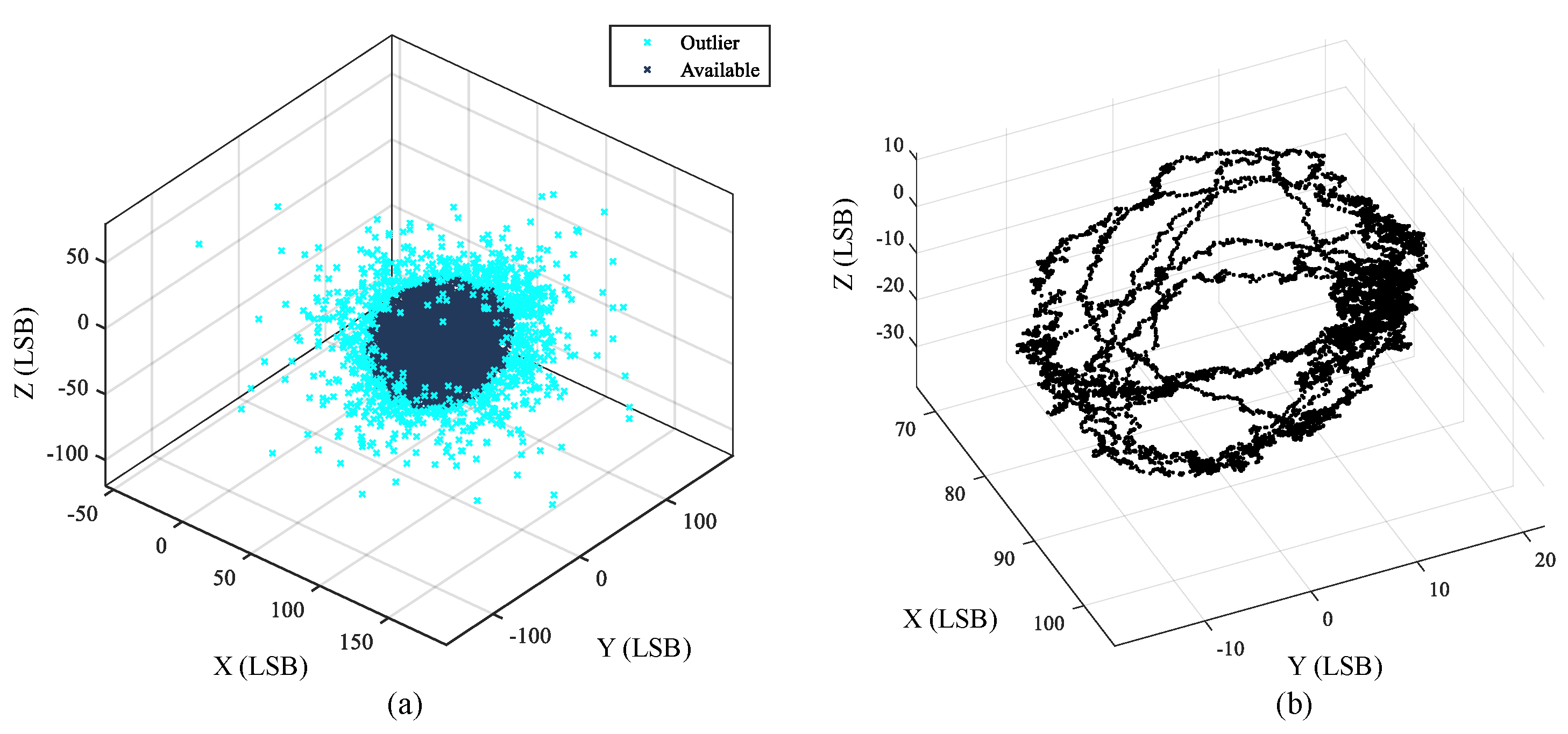
• Import the collected data into the computer and detect the outliers by adopting the GMM binary classification method, as shown in Figure 8a. The data points are divided into two classes, and the class dissociated from the center is labeled the outlier class.
• Adpot a sliding mean filter using MATLAB to reduce the error caused by ADC sampling jitter, as shown in Figure 8b.
• Fit the data points by the least squares method and obtain a fitted ellipsoid from Equation (7) and its parameters, as shown in Figure 9a.
• Calculate all parameters of the compensation matrix ${\left({\mathit{C}}_s{\mathit{C}}_v\right)}^{-1}$ according to Equation (8) to calibrate the three-axis magnetic sensor.
• Calculate the original data points through the compensation matrix ${\left({\mathit{C}}_s{\mathit{C}}_v\right)}^{-1}$ to obtain calibrated data. Use the least squares method to fit the ellipsoid and calculate the ellipsoid’s parameters, as shown in Figure 9b.

The ellipsoidal parameters are compared before and after calibration.

Before calibration, the coordinates of the ellipsoid’s center are (85.393, 0.63924, −9.6124), and the radii are $19.718, 18.415,$ and $13.529$. After calibration, the coordinates of the ellipsoid’s center are (−0.26683, −0.019272, −0.050791), and the radii are $18.016, 17.344$ and $16.971$. The center of the ellipsoid is closer to the origin, and the eccentricity is decreased, which indicates that the accuracy of the TMR sensor is improved after calibration.

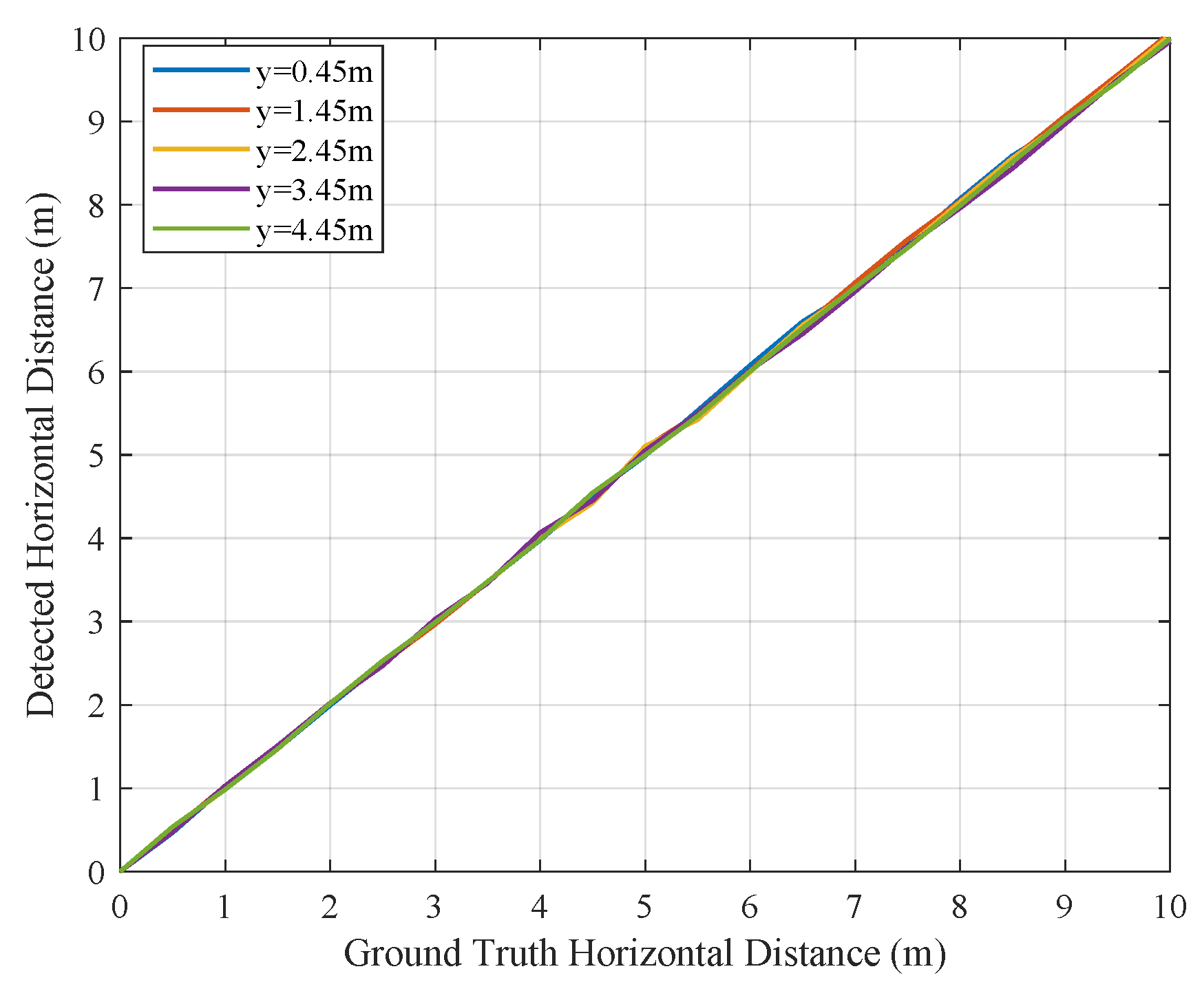
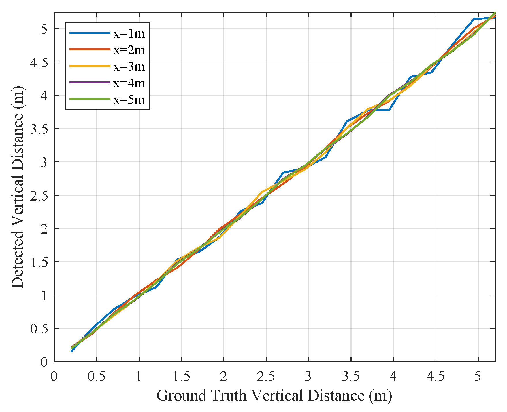
4.2. Three-Dimensional Pipeline Location Simulation

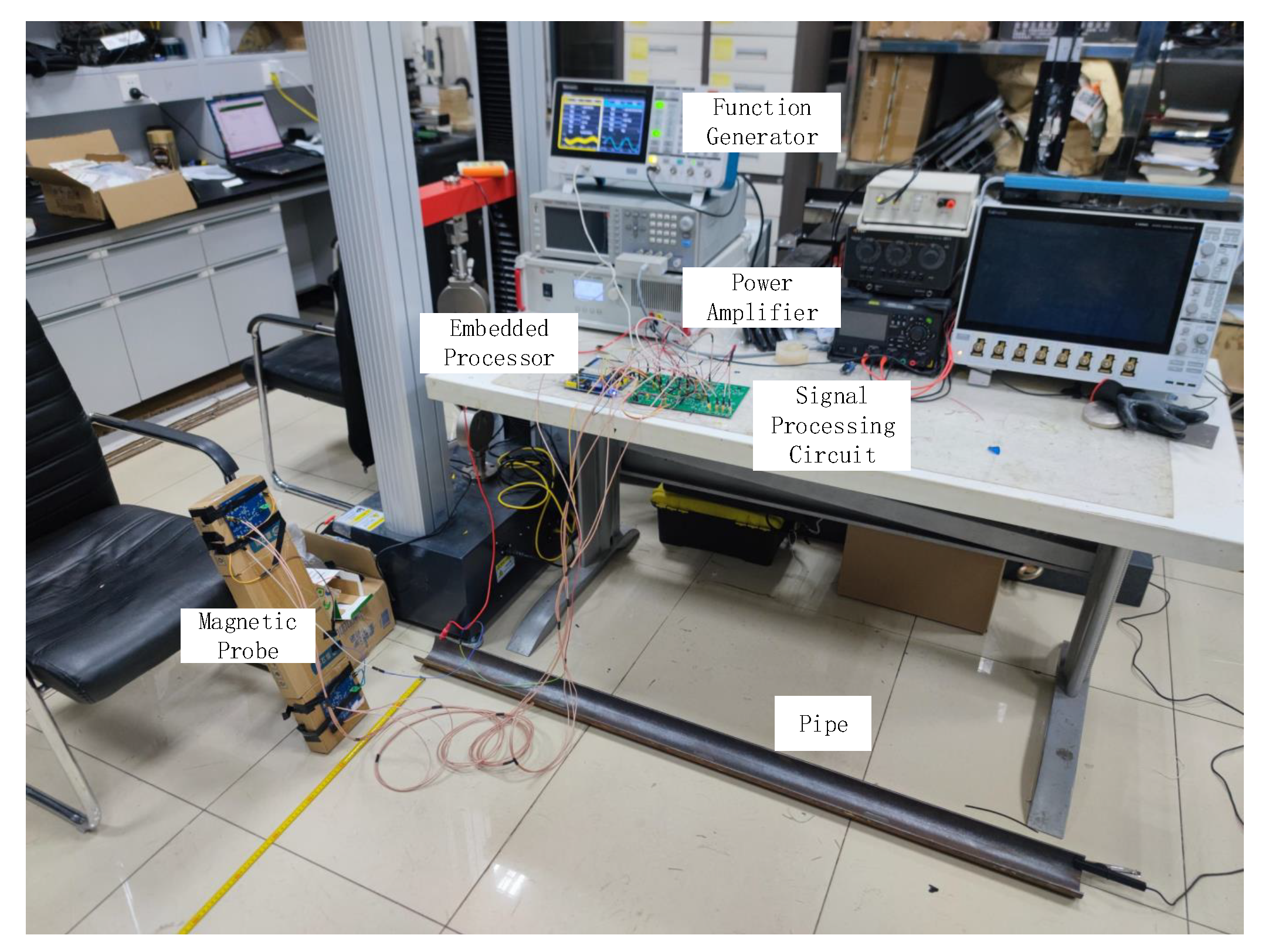
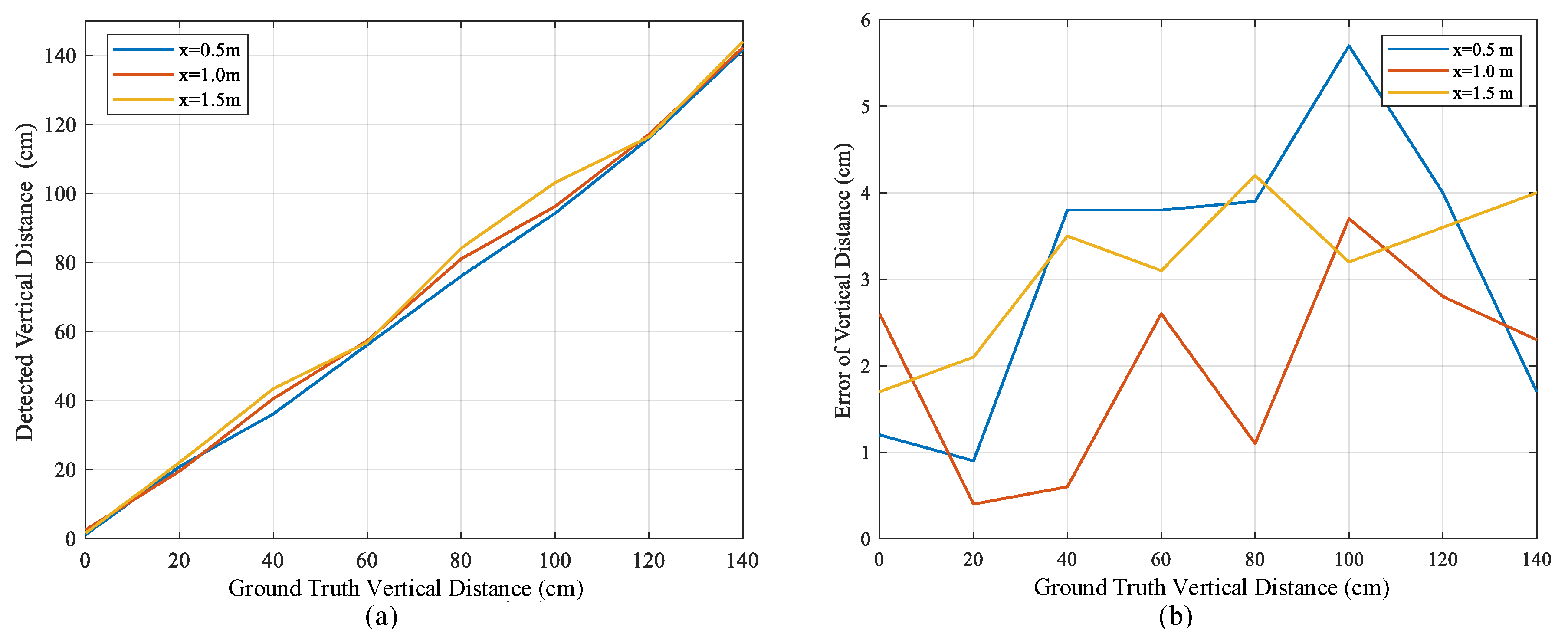
In order to verify the correctness of the three-dimensional pipeline position location method, a three-dimensional simulation model was built in COMSOL Multiphysics, as shown in Figure 10. The length, width, and height of the model were 4 m, 10 m, and 10 m, respectively. The upper part was the air domain, the bottom part was the pipeline and soil domain, the buried depth of the pipeline was 1 m, and the infinite element domain was arranged in the outer boundary of the whole model. In the pipeline, the input frequencies were 4 Hz, 8 Hz, and 72 Hz, while the RMS value was 0.5 A. The specific parameters of each material in the model are shown in

Table 2. The specific parameters of materials.

Material	Relative Magnetic Conductivity	Relative Dielectric Constant	Specific Conductance (S/m)
Air	1	1	0
Iron	1	1	$4.032$ × ${10}^6$
Soil	0.975	2.6	$1.70$ × ${10}^{-4}$

.

The magnetic induction probes in the Y-axis direction were placed at x-coordinates of −2 m and 2 m, and the Y-axis components of the magnetic induction were detected at these two locations, as shown in Figure 11. The magnetic induction intensity consisted of signals with frequencies of 4 Hz, 8 Hz and 72 Hz, and the amplitude was around $1.3\times {10}^{-7}$ T.

In order to verify the correctness of the relative pipeline position location method, a MATLAB processing program was compiled. To calculate the phase difference, reference signals with the same phase at 4 Hz and 8 Hz were generated. Compared with the different frequency signals obtained by the simulation, the phase difference relative to the reference signal was calculated and converted to the time difference relative to the reference signal. The relative position of the pipeline was able to be determined. The process is shown in Figure 12.

The simulation signals on the right and the left side, which are shown in Figure 11, were imported into MATLAB and analyzed by the program above. The FFT analysis results are shown in Figure 13. The amplitude of the signal with different frequencies are shown in the amplitude spectra, and the phases of different frequencies are shown in the phase spectra. It can be seen in Figure 13a that the amplitudes of the signals at 4 Hz, 8 Hz, and 72 Hz are about $4.57\times {10}^{-8}$ T, and their phases are −83°, −75° and −140.3°, respectively. The lag time $\Delta t$ between the signals at 4 Hz and 8Hz is 0.0001 s according to Equation (11). Figure 13b shows that the amplitudes of the signals at 4 Hz, 8 Hz, and 72 Hz are about $5.01\times {10}^{-8}$ T, and their phases are 97°, 104.3°, and 39.6°, respectively. The lag time $\Delta t$ between the signals at 4 Hz and 8 Hz is 0.0624 s.

The relative position of the pipeline is located using the lag time between the 4 Hz and 8 Hz signals. Figure 13a illustrates that the program determines that the pipeline is on the left for $\Delta t<1/32$. Figure 13b illustrates the program determines that the pipeline is on the right for $\Delta t>1/32$, which is consistent with the actual situation.

In order to evaluate the accuracy of the calculation of the horizontal and vertical distances, two sets of three-dimensional magnetic induction probes with 0.5 m vertical intervals were placed in the model at 1 m intervals in the horizontal and vertical directions. The horizontal distance and vertical distance were calculated according to Equations (19) and (20), and the results are shown in Figure 14 and Figure 15. In Figure 14, the X-axis represents the ground-truth horizontal distance between the probe and the pipeline, and the Y-axis represents the measured horizontal distance, both of which are in meters. In Figure 15, the X-axis represents the the ground-truth vertical distance between the probe and the pipeline, and the Y-axis represents the measured vertical distance, both of which are in meters.

In order to evaluate the accuracy of the horizontal angle measurements between the positive direction of the probe and the pipeline, the model was rotated in the horizontal direction at intervals of 10°. The horizontal angle was calculated according to Equation (21), and the results are shown in Figure 16, where, the X-axis represents the the ground-truth horizontal angle between the positive direction of the probe and the pipeline and the Y-axis represents the measured horizontal angle; both are presented in degrees.

4.3. Experiment

4.3.1. Experiment Design

The function generator Tektronix AFG31102 was adopted to generate multi-frequency currents at 4 Hz, 8 Hz, and 72 Hz and output the signal to the Aigtek ATA-308 power amplifier. After adjusting the RMS value of the output current to 1A, it was transmitted into the pipeline model through a shielded cable to simulate the pipeline detection environment in a practical scene. A schematic diagram of the test platform is shown in Figure 17.

The detection probe is shown in Figure 18. During the experiment, the probe kept a plumb relationship with the ground, and the horizontal distance, vertical distance, and horizontal angle between the probe and the pipeline changed. The magnetic field signal emitted by the pipeline was detected by the detection probe. The signal was filtered and amplified by the signal-processing circuit and transmitted to the STM32F429 embedded processor to calculate its accurate three-dimensional position. The processed pipeline positioning results were displayed through the LCD. The test environment and test equipment are shown in Figure 19 and Figure 20.

4.3.2. Experimental Results

In order to evaluate the correctness of the theoretical model, horizontal angle measurement, horizontal distance measurement, and vertical distance measurement experiments were carried out.

In Figure 21a, the X-axis represents the ground-truth horizontal angle between the positive direction of the probe and the pipeline, and the Y-axis represents the measured horizontal angle; both axes are in degrees. In the horizontal angle measurement experiment, the probe was 1 m from the pipeline in the vertical axis, and the horizontal distance was 0.5 m, 1.0 m, and 1.5 m, respectively. The measurement range was 0°–90°, and the step length was 10°. The error of the horizontal angle measurements is shown in Figure 21b. When the horizontal distance was 0.5 m, the measurement had the minmum error.

In Figure 22a, the X-axis represents the ground-truth horizontal distance between the probe and the pipeline, and the Y-axis represents the measured horizontal distance and its error; both axes are in cm. In the horizontal distance measurement experiment, the angle between the positive direction of the probe and the pipeline was 0°, and the height from the pipeline was 0.5 m, 1.0 m, and 1.5 m, respectively. The measurement range was 0–100 cm, and the step size was 10 cm. The error of the horizontal distance measurement is shown in Figure 22b. When the height from the pipeline was 1.5 m, the measurement had the maximum error.

In Figure 23a, the X-axis represents the ground-truth vertical distance between the probe and the pipeline, and the Y-axis represents the measured vertical distance; both axes are in cm. In the vertical distance measurement experiment, the angle between the positive direction of the probe and the pipeline was 0°, and the horizontal distance from the pipeline was 0.5 m, 1.0 m, and 1.5 m. The measurement range was 0–140 cm, and the step size was 20 cm. The error of the vertical distance measurement is shown in Figure 23b. When the horizontal distance from the pipeline was 1.5 m, the measurement had the maximum error.

The average error and $R^2$ of the test results are shown in

Table 3. Experimental results.

Object	Variable (m)	${\mathit{R}}^2$	Average Error
Angle (°)	0.5	0.9953	1.85°
	1	0.9822	3.67°
	1.5	0.9935	2.51°
Horizontal Distance (cm)	0.5	0.9937	2.39 (cm)
	1	0.9975	2.19 (cm)
	1.5	0.9953	3.14 (cm)
Vertical Distance (cm)	0.5	0.9966	3.12 (cm)
	1	0.9977	2.01 (cm)
	1.5	0.996	3.17 (cm)

. The results show satisfactory linearity in the angle, horizontal, and vertical distance measurement experiments. However, with increased distance in three dimensions, especially the horizontal distance, the measurements are increasingly negatively affected. However, the measurement results are consistent with the theory and can meet our factual needs.

5. Conclusions

In this paper, a TMR-array-based pipeline location method is proposed. Firstly, in order to detect the magnetic field and locate the pipeline accurately, a detection probe is redesigned using a TMR array. Secondly, an improved calibration method for the TMR array based on the GMM binary classification method is proposed, which reduces the influence of ADC sampling noise on the calibration parameters. In addition, a relative pipeline position location method is proposed based on the relationship of the lag time with different frequency signals. Thirdly, the magnetic induction intensity is studied at various positions around the pipeline, and a three-dimensional pipeline location method is proposed, which is equipped to calculate the horizontal and vertical distance and the horizontal angle between the detection probe and the pipeline. Fourthly, TMR2705 single-axis magnetic sensors are adopted to constitute a TMR array. The collected data are calibrated using the calibration method above. Experiments are carried out to verify the correctness of the calibration method. Fifthly, COMSOL Multiphysics is adopted to build a simulation model, and the correctness of the three-dimensional pipeline location method is verified. Finally, a hardware circuit is designed, and a test platform is built. Experiments measuring the horizontal and vertical distances and the horizontal angle are carried out by simulating practical scenes. The indexes of the average error and linearity are satisfactory, the $R^2$ of the horizontal distance and the vertical distance measurement proves to be greater than 0.99, and the $R^2$ of the horizontal angle measurement is greater than 0.98, which verifies the feasibility of the method above from the perspective of the experiment.

By using a TMR array and designing a signal-processing circuit, this paper realizes the accurate measurement of magnetic field signals around the pipeline. It identifies the accurate three-dimensional location of a pipeline at a low cost without the assistance of other equipment. This method reduces the shortcomings of PCM, which can only determine the general direction of the pipeline.

Since specified frequency magnetic field signals are adopted in the pipeline location process, the proposed method might be less affected by magnetic signals in the practical environment. In the future, we will endeavor to combine this method with an inspection robot outside the pipeline to improve the efficiency of pipeline inspection in the practical environment. We aim to carry these experiments out after finding suitable experimental facilities.

References

1. Jacobi, M.; Karimanzira, D. Underwater pipeline and cable inspection using autonomous underwater vehicles. In Proceedings of the 2013 MTS/IEEE OCEANS—Bergen, Bergen, Norway, 10–14 June 2013. [Google Scholar]
2. Kandroodi, M.R.; Araabi, B.N.; Ahmadabadi, M.N.; Shirani, F.; Bassiri, M.M. Detection of natural gas pipeline defects using magnetic flux leakage measurements. In Proceedings of the 2013 21st Iranian Conference on Electrical Engineering (ICEE), Mashhad, Iran, 14–16 May 2013. [Google Scholar]
3. Lu, S.; Yue, Y.; Liu, X.; Wu, J.; Wang, Y. A novel unbalanced weighted KNN based on SVM method for pipeline defect detection using eddy current measurements. Meas. Sci. Technol. 2022, 34, 014001. [Google Scholar] [CrossRef]
4. Wang, Y.; Su, C.; Xie, M. Optimal inspection and maintenance plans for corroded pipelines. In Proceedings of the 2021 Global Reliability and Prognostics and Health Management (PHM-Nanjing), Nanjing, China, 15–17 October 2021; pp. 1–6. [Google Scholar] [CrossRef]
5. Liu, X.; Zheng, J.; Fu, J.; Nie, Z.; Chen, G. Optimal inspection planning of corroded pipelines using BN and GA. J. Pet. Sci. Eng. 2018, 163, 546–555. [Google Scholar] [CrossRef]
6. Liu, B.; Lian, Z.; Liu, T.; Wu, Z.; Ge, Q. Study of MFL signal identification in pipelines based on non-uniform magnetic charge distribution patterns. Meas. Sci. Technol. 2023, 34, 044003. [Google Scholar] [CrossRef]
7. Pasha, M.A.; Khan, T.M. A pipeline inspection gauge based on low cost magnetic flux leakage sensing magnetometers for non-destructive testing of pipelines. In Proceedings of the 2016 International Conference on Emerging Technologies (ICET), Islamabad, Pakistan, 18–19 October 2016. [Google Scholar]
8. Chen, W.; Ma, F. The application of the risk-based inspection technique in the failure possibility analysis of the buried gas pipeline. In Proceedings of the 2009 16th International Conference on Industrial Engineering and Engineering Management, Beijing, China, 21–23 October 2009; pp. 1308–1311. [Google Scholar]
9. Liu, X.; Hu, C.; Peng, P.; Li, R.; Zheng, D.Z. In-pipe Detection System Based on Magnetic Flux Leakage and Eddy Current Detection. In Proceedings of the 2020 International Conference on Sensing, Measurement & Data Analytics in the Era of Artificial Intelligence (ICSMD), Xi’an, China, 15–17 October 2020. [Google Scholar]
10. Li, S.; Huang, R.; Xu, W.; Zuo, Z.; Liang, S. Unsupervised leak detection of natural gas pipe based on leak-free flow data and deep auto-encoder. In Proceedings of the 2022 China Automation Congress (CAC), Xiamen, China, 25–27 November 2022; pp. 678–683. [Google Scholar] [CrossRef]
11. Li, X.; Ma, L.; Liu, L.; Dai, J.; Zhang, H.; Liang, J.; Liang, S. A Leak Detection Algorithm for Natural Gas Pipeline Based on Bhattacharyya Distance. In Proceedings of the 2021 International Conference on Advanced Mechatronic Systems (ICAMechS), Tokyo, Japan, 9–12 December 2021; pp. 33–36. [Google Scholar] [CrossRef]
12. Akinsete, O.; Oshingbesan, A. Leak Detection in Natural Gas Pipelines Using Intelligent Models. In Proceedings of the SPE Nigeria Annual International Conference and Exhibition, Lagos, Nigeria, 5–7 August 2019. [Google Scholar]
13. Sheltami, T.R.; Bala, A.; Shakshuki, E.M. Wireless sensor networks for leak detection in pipelines: A survey. J. Ambient. Intell. Humaniz. Comput. 2016, 7, 347–356. [Google Scholar] [CrossRef]
14. Extended Abstract for Presenting the Pipeline Current Mapper Solution at NACE, Vol. All Days. In Proceedings of the AMPP Annual Conference + Expo, AMPP-2022-17617, San Antonio, TX, USA, March 2022.
15. Li, R. Urban Underground Pipeline Measurement and Automatic Mapping. Master’s Thesis, North China University of Science and Technology, Qinhuangdao, China, 2019. [Google Scholar]
16. Technology of Detecting Deep Underground Metal Pipeline by Magnetic Gradient Method. IOP Conf. Ser. Earth Environ. Sci. 2021, 7, 390–393.
17. Zhao, Y.; Wang, X.; Sun, T.; Chen, Y.; Yang, L.; Zhang, T.; Ju, H. Non-contact harmonic magnetic field detection for parallel steel pipeline localization and defects recognition. Measurement 2021, 180, 109534. [Google Scholar] [CrossRef]
18. Velázquez, J.C.; Hernández-Sánchez, E.; Terán, G.; Capula-Colindres, S.; Diaz-Cruz, M.; Cervantes-Tobón, A. Probabilistic and Statistical Techniques to Study the Impact of Localized Corrosion Defects in Oil and Gas Pipelines: A Review. Metals 2022, 12, 576. [Google Scholar] [CrossRef]
19. Velázquez, J.C.; Caleyo, F.; Valor, A. Predictive Model for Pitting Corrosion in Buried Oil and Gas Pipelines. Corros. J. Sci. Eng. 2009, 65, 332–342. [Google Scholar] [CrossRef]
20. Fang, X.; Deng, J. Detection of Deep Pipeline. In Proceedings of the 20th Annual of the Chinese Geophysical Society, Xi’an, China, 16–20 October 2003. [Google Scholar]
21. Tian, W.M. Integrated method for the detection and location of underwater pipelines. Appl. Acoust. 2008, 69, 387–398. [Google Scholar] [CrossRef]
22. Hongzhi, W.; Jinghe, C.; Kaifeng, L.; Xin, G.; Zidong, Z. Improved Correction Method of Signal Values Based on One-pass System. In Proceedings of the CORROSION, San Antonio, TX, USA, 9–13 March 2014. [Google Scholar]
23. Nadimi, N.; Javidan, R.; Layeghi, K. Efficient Detection of Underwater Natural Gas Pipeline Leak Based on Synthetic Aperture Sonar (SAS) Systems. J. Mar. Sci. Eng. 2021, 9, 1273. [Google Scholar] [CrossRef]
24. Jinnah Sheik Mohamed, A.B.; Venusamy, K.; Sangeetha, S.; Abdullah Al Rawahi, A.S.; Said Mahmood Al Balushi, A. Leak Detection and Corrosion Identification in Water Tubes, Gas Pipes by Mobile Robot. In Proceedings of the 2021 2nd International Conference on Smart Electronics and Communication (ICOSEC), Trichy, India, 7–9 October 2021; pp. 1–6. [Google Scholar] [CrossRef]
25. Roskosz, M. Metal magnetic memory testing of welded joints of ferritic and austenitic steels. NDT & E Int. 2011, 44, 305–310. [Google Scholar]
26. Chen, Z.; Dang, R.; Xie, R. Research on electromagnetic Detection Technology of underground metal pipeline. Electron. Test 2017, 15, 50–51. [Google Scholar]
27. Yang, Q.; Yang, J.; Liu, W. Application of current method in multi—Frequency tube in buried pipeline detection. Chem. Mach. 2017, 44, 6. [Google Scholar]
28. Liu, S.; Ren, X.; Qiao, H. Design of constant current transmitter for underground pipeline detection system based on PCM. Int. Electron. Elem. 2023, 31, 8. [Google Scholar]
29. Tuo, Y. Research and Design of Intelligent Cable Path Detector. Master’s Thesis, Xidian University, Xi’an, China, 2009. [Google Scholar]
30. Li, Q.; Li, Z.; Zhang, Y.; Fan, H.; Yin, G. Integrated Compensation and Rotation Alignment for Three-Axis Magnetic Sensors Array. IEEE Trans. Magn. 2018, 54, 4001011. [Google Scholar] [CrossRef]
31. Xueyuan, L.; Yulin, C.; Min, Z. Error Analysis and Compensation of Three-axis Strap-down Magnetometers. In Proceedings of the 2007 8th International Conference on Electronic Measurement and Instruments, Xi’an, China, 16–18 August 2007; pp. 1-294–1-297. [Google Scholar] [CrossRef]
32. Hu, F.; Wu, Y.; Yu, Y.; Nie, J.; Li, W.; Gao, Q. An Improved Method for the Magnetometer Calibration Based on Ellipsoid Fitting. In Proceedings of the 2019 12th International Congress on Image and Signal Processing, BioMedical Engineering and Informatics (CISP-BMEI), Suzhou, China, 19–21 October 2019; pp. 1–5. [Google Scholar] [CrossRef]
33. Fang, J.; Sun, H.; Cao, J.; Xiao, Z.; Ye, T. A Novel Calibration Method of Magnetic Compass Based on Ellipsoid Fitting. IEEE Trans. Instrum. Meas. 2011, 60, 2053–2061. [Google Scholar] [CrossRef]
Figure 1. The flowchart of the method.
Sustainability 15 09816 g001
Figure 2. The device and principle of PCM. (a) The principle of PCM. (b) The practical device called a PCM. Here, (1) represents the pipeline test pile, (2) represents the high-power signal transmitter, (3) represents the transmitter’s ground point, and (4) represents the PCM receiving equipment.
Sustainability 15 09816 g002
Figure 3. The PCM probe structure.
Sustainability 15 09816 g003
Figure 4. The non-orthogonal error.
Sustainability 15 09816 g004
Figure 5. The detection probe.
Sustainability 15 09816 g005
Figure 6. The theory of detection probe. Δ h represents the distance between the two TMR arrays, h represents the vertical distance between the bottom sensors and the pipe, M represents the position of the upper sensors, N represents the position of the bottom sensors, A x , A y , and A z represent the amplitude of signals detected from the bottom sensors, and A x , A y , and A z represent the amplitude of signals detected from the upper sensors.
Sustainability 15 09816 g006
Figure 7. The TMR array.
Sustainability 15 09816 g007
Figure 8. Data pre-processing. (a) GMM binary classification. (b) Sliding mean filter.
Sustainability 15 09816 g008
Figure 9. The ellipsoid after fitting. (a) Before calibration. (b) After calibration.
Sustainability 15 09816 g009
Figure 10. The three-dimensional simulation model.
Sustainability 15 09816 g010
Figure 11. The Y-axis components of the magnetic induction.
Sustainability 15 09816 g011
Figure 12. The script of the relative pipeline position location method.
Sustainability 15 09816 g012
Figure 13. The FFT analysis of signals on both sides. (a) On the left side. (b) On the right side.
Sustainability 15 09816 g013
Figure 14. Horizontal distance measurement simulation.
Sustainability 15 09816 g014
Figure 15. Vertical distance measurement simulation.
Sustainability 15 09816 g015
Figure 16. Horizontal angle measurement simulation.
Sustainability 15 09816 g016
Figure 17. Schematic diagram of the experimental platform.
Sustainability 15 09816 g017
Figure 18. Magnetic signal detection probe.
Sustainability 15 09816 g018
Figure 19. Experimental platform.
Sustainability 15 09816 g019
Figure 20. Signal-processing circuit.
Sustainability 15 09816 g020
Figure 21. Horizontal angle measurement experiment. (a) Horizontal angle measurement. (b) Error of horizontal angle measurement.
Sustainability 15 09816 g021
Figure 22. Horizontal distance measurement experiment. (a) Horizontal distance measurement. (b) Error of horizontal distance measurement.
Sustainability 15 09816 g022
Figure 23. Vertical distance measurement experiment. (a) Vertical distance measurement. (b) Error of vertical distance measurement.
Sustainability 15 09816 g023