A Novel Numerical Method for Geothermal Reservoirs Embedded with Fracture Networks and Parameter Optimization for Power Generation

Abstract

Geothermal recovery involves a coupled thermo-hydro-mechanical (THM) process in fractured rocks. A fluid transient equilibrium equation, considering thermal conduction, convection, and heat exchange, is established. The evolution of the reservoir permeability and the variance in the fracture aperture due to a change in the stress field are derived simultaneously. THM coupling is accomplished through iterative hydromechanical and thermo-hydro processes. To overcome the difficulty of geometric discretization, a three-dimensional THM coupler model embedded with discrete fracture networks, using a zero-thickness surface and line elements to simulate fractures and injection/production wells, is established to evaluate the geothermal production. The reliability of the method is verified by a case study. Then, this method is applied to evaluate the influence of the geometric topological characteristics of fracture networks and the fracture aperture on the reservoir temperature evolution and heat extraction effectiveness. The results show that the power generation efficiency and geothermal depletion rate are significantly affected by the injection–production pressure. Injection wells and production wells with pressures higher than the initial fluid pressure in the fractures can be used to significantly increase power generation, but the consumption of geothermal energy and loss of efficiency are significant and rapid. To achieve better benefits for the geothermal recovery system, an optimization algorithm based on simultaneous perturbation stochastic approximation (SPSA) is proposed; it takes the power generation efficiency as the objective function, and the corresponding program is developed using MATLAB to optimize the position and pressure values for each production well. The results show that the heat transfer for the entire EGS reservoir becomes more uniform after optimization, and the heat transfer efficiency is greatly improved.

1. Introduction

The large amounts of heat stored in hot sedimentary aquifers (HSAs) worldwide have attracted increasing attention due to their renewability and cleanliness [1,2]. Geothermal recovery is a multiphysics coupled process in which the stress, thermal, and flow fields interact [3,4]. Hot dry rock is located deep underground, with low porosity and permeability. Hydraulic fracturing is an effective method of increasing reservoir permeability [5]. Therefore, proper evaluation of the increased permeability of rock mass due to the fracture network is a prerequisite for designing a valuable hydraulic fracturing scheme [6,7]. Establishing a mathematical model of a thermo-hydro-mechanical coupled (THM) system and performing numerical simulations for enhanced geothermal systems (EGS) is an economical and efficient way to analyze geothermal resource recovery [8,9,10]. The equivalent continuum model and the discrete fracture network model are two models widely used in geothermal recovery analyses [11,12,13,14]. The equivalent continuum model considers fractures and the rock matrix as a homogeneous medium, with the seepage and heat transfer effects acting uniformly over the entire research domain [15,16]. Although the equivalent continuum model is simple and convenient, it cannot be used to describe the transfer and exchange of fluid and thermal energy between different media, and ignores the complex distribution characteristics of fractures in the rock mass [17,18]. The discrete fracture network model considers that the rock mass to be composed of a rock matrix and fracture networks, which is closer to the actual reservoir and can be used to characterize the hydrothermal migration process more realistically [19]. However, the dimensional difference for fractures in three directions brings challenges to geometric discretization and numerical calculation for geothermal reservoir models embedded with fracture networks [20,21]. In addition, the number of fractures is large, and their distribution is dense. It is difficult to simulate the coupled process of seepage and heat transfer with a three-dimensional discrete fracture network model [22,23]. In total, the main difficulty in geothermal recovery simulation lies in how to effectively consider the seepage and heat transfer between the fracture, rock matrix, and well; there is a need to overcome the drawback of grid discretization and compute a governing equation for a large number of 3D rock fractures [24,25,26].

It is difficult to explore hot dry rock, and investment in geothermal recovery systems is large. Therefore, evaluating the commercial potential of EGSs has attracted increasing attention. In the process of EGS geothermal recovery, the fluid mainly flows along the dense fracture area due to the uneven distribution of fractures, the fluid cannot conduct sufficient heat exchange with the reservoir, and the enhanced geothermal reservoir cannot be fully recovered [1,27]. Some research has found that deploying more production wells does not necessarily improve the heat extraction capacity of EGSs during long-term geothermal recovery, while a reasonable location arrangement for wells and production pressure can ensure maximum efficiency for geothermal recovery [28,29]. For above-ground power systems, transcritical and multipressure subcritical organic Rankine cycles (ORC) are the optimal power generation configurations for EGS system [30,31]. To fully assess the commercial potential of an EGS system, researchers often use specialized economic models, such as the levelized cost of electricity (LCOE) and payback period (PBP), to evaluate the performance of a system [32,33]. Geothermal recovery and power generation systems are two interdependent production processes. It is necessary to combine HDR geothermal recovery with a ground-based power generation configuration, optimize the dynamic performance of an EGS over its entire life cycle, and filter out the most suitable system configuration and the best operating conditions corresponding to different seasons.

In the present study, the mathematical expression for thermo-hydro-mechanical (THM) coupling is derived and transferred into COMSOL to simulate the geothermal recovery. An equivalent simulation method for the three-dimensional seepage heat transfer coupling of a fractured rock mass is proposed, where fractures are represented by surface elements, the rock matrix is considered an equivalent continuous medium, and injection/producer wells are represented by line elements. The effectiveness of the method is verified by comparison with the simulation method, without geometric simplification. Finally, the method is applied to the numerical simulation of a geothermal recovery system with large-scale complex fracture networks, and methods to optimize the position of the production well and the hydraulic pressure of the injecting/production well are proposed.

2. Materials and Methods Governing Equations for Fluid Flow and Heat Transfer

2.1. Fluid Flow in the Fracture and Rock Matrix

The fluid flow through the fracture conforms to the following governing equation [34,35]:

$$d_f{s}_f\frac{\partial p}{\partial t}+{\nabla }_{\tau }\left(-\frac{k_f}{\eta }{d}_f{\nabla }_{\tau }p\right)=Q_f$$

(1)

where $d_f$ is the fracture aperture, m; $s_f$ is the water storage coefficient of the fracture, 1/Pa; $k_f$ is the permeability of the fracture, m²; and $Q_f$ is the fluid flowing from the matrix to the fracture, m/s, which conforms to the following formula:

$$Q_f=-\frac{k_f}{\eta }\frac{\partial p}{\partial n}$$

(2)

where $\partial p/\partial n$ represents the gradient of hydraulic pressure along the normal direction of the fracture surface. The above conclusions are available only when the fracture surface’s aperture is constant, and fracture is considered two smooth plates separated by a small distance. Indeed, the fracture surface is rough, and the permeability of the fracture in engineering should be rectified using a revision coefficient $\xi$:

$$k_f=\frac{\xi d_f^2}{12}$$

(3)

The fluid flow in the rock matrix follows Darcy’s law:

$$s_m\frac{\partial p}{\partial t}+\nabla u=Q$$

(4)

$$u=-\frac{k_m}{\eta }\nabla p$$

(5)

where $s_m$ is the water storage coefficient of the rock matrix, 1/Pa; $p$ is the water pressure; $t$ is the time, s; $u$ is the flow velocity of water, m/s; and $k_m$ is the permeability of the rock matrix, m².

2.2. Heat Transport in the Fracture and Rock Matrix

Considering that the flow velocity is large in fractures, heat storage and diffusion can be negligible compared with thermal advection. Therefore, according to the conservation of heat, the heat transfer in the fracture conforms to the following expressions [36]:

$${\rho }_f{c}_f\frac{\partial T_f}{\partial t}+{\rho }_f{c}_f{u}_f{\nabla }_{\tau }{T}_f=-{\nabla }_{\tau }\left({\lambda }_m{\nabla }_{\tau }{T}_m\right)+W$$

(6)

$${\rho }_m{c}_m\frac{\partial T_m}{\partial t}+{\rho }_m{c}_m{u}_m{\nabla }_{\tau }{T}_m={\nabla }_{\tau }\left({\lambda }_f{\nabla }_{\tau }{T}_f\right)+\frac{W_f}{d_f}$$

(7)

where $T$ is temperature, K; $\lambda$ is the heat transfer coefficient, w/(m·K); c is the specific heat capacity, J/(kg·k); and $W$ is the heat source, w/m³. The subscript $f$ represents the fracture, the subscript $m$ represents the matrix, and $W_f$ is the heat absorbed by the fracture from the matrix, which is calculated from

$$W_f=h\left(T_m-T_f\right)$$

(8)

where $h$ is the heat transfer coefficient, w/(m²·K).

3. Thermo-Hydromechanical Analysis in an EGS

3.1. Evolution of Porosity and Permeability in a Porous Matrix

The porosity of a geothermal reservoir is defined as follows [37]:

$$\phi =\frac{v_0-v_s}{v_0}$$

(9)

where $v_0$ is the volume of material in the natural state and $v_s$ is the compact volume of the material. Defining $d{v}_0$ as the increment in $v_0$, $d{v}_s$ is the increment in $v_s$, and the variance of porosity can be derived from Equation (9):

$$\left(\frac{v_0}{v_s}+\frac{d{v}_0}{v_s}\right)d\phi =-\frac{d{v}_s}{v_s}+\frac{d{v}_0}{v_0}$$

(10)

The volume strain of the thermal reservoir may be negligible, considering the restriction by the surrounding rock mass; therefore, Equation (10) can be written as

$$\frac{1}{1-\phi }d\phi =-\frac{d{v}_s}{v_s}$$

(11)

The changes in the volume of the rock skeleton due to changes in fluid pressure and temperature are represented by $d{v}_{sp}/v_s$ and $d{v}_{sT}/v_s$, respectively. Then, the strain increment for the rock skeleton can be expressed as

$$\frac{d{v}_s}{v_s}=\frac{d{v}_{sp}}{v_s}+\frac{d{v}_{sT}}{v_s}$$

(12)

In Equation (12):

$$d{v}_{sp}=\frac{v_s}{k_s}dp\hspace{1em}\mathrm{and}\hspace{1em}d{v}_{sT}=v_s{\alpha }_T{d}_T$$

(13)

Substituting Equation (13) into Equation (12) gives

$$\frac{d{v}_s}{v_s}=-\frac{1}{k_s}+{\alpha }_T{d}_T$$

(14)

where $k_s$ is the bulk modulus of the rock skeleton and ${\alpha }_T$ is the thermal expansion coefficient of the rock skeleton. The function of porosity $\phi$ can be obtained by substituting Equation (14) into Equation (11):

$$\phi =1-\left(1-{\phi }_0\right)\times \exp \left[1-\frac{1}{k_s}\left(p-p_0\right)+{\alpha }_T\left(T-T_0\right)\right]$$

(15)

where $T$ is the current temperature; $T_0$ is the initial temperature; $p$ is the initial pore pressure of the rock matrix; $p_0$ is the current pore pressure of the rock matrix; and ${\phi }_0$ is the initial porosity of the rock matrix. Based on the Kozeny–Carman equation, the hydraulic permeability of reservoir matrices with different porosities can be expressed as follows [38]:

$$\frac{k}{k_0}={\left(\frac{\phi }{{\phi }_0}\right)}^3$$

(16)

where $k$ is the current rock permeability and $k_0$ is the initial rock permeability. Combining Equation (15) with Equation (16) yields

$$k=k_0{\left\{\frac{1}{{\phi }_0}-\left(\frac{1}{{\phi }_0}-1\right)\times \exp \left[-\frac{1}{k_s}\left(p-p_0\right)+{\alpha }_T\left(T-T_0\right)\right]\right\}}^3$$

(17)

3.2. THM Model for the Evolution of the Fracture Aperture

Many attempts have been made to model the relationship between stress and the fracture aperture, e.g., in linear, exponential, and logarithmic functions. Among them, the exponential relationship is widely applied and is used in this study [39]:

$$b_m=b_{mr}+\left(b_{m0}-b_{mr}\right)\times \exp \left(-\alpha ·\sigma \right)$$

(18)

where $b_m$, $b_{mr}$, $b_{m0}$, $\alpha$, and $\sigma$ are the apertures created by mechanical effects, the residual aperture, the aperture under initial stress, and a constant depending on the nonlinear stiffness of the fracture and the applied stress, respectively. It should be noted that the difference between $b_{m0}$ and $b_{mr}$ is the maximum deformation of the aperture $b_{max}$. Fractures are affected by external stress, thermal stress, and hydraulic pressure, and the fracture aperture is enhanced as follows [40]:

$$b=b_r+b_{max}\times \exp \left(-\alpha ·\sigma \right)\times \exp \left\{-\left(\beta -\frac{\gamma }{T}\right)\sigma \right\}$$

(19)

where $b$ is the fracture aperture and $\alpha$, $\beta$ and $\gamma$ are empirical constants that can be used to characterize the dependence of the fracture aperture on stress, chemistry, and temperature, respectively.

With a reduction in hydraulic pressure or a decrease in temperature, the fracture aperture increases. Nevertheless, the fracture aperture cannot be fully recovered considering the irreversible plastic deformation and removal of material peeled from the contact surface [41]. Therefore, there exists a ratio $R\left(R<1\right)$ between the recovered maximum aperture $b_{max}^u$ and the maximum aperture $b_{max}$:

$$R=\frac{b_{max}^u}{b_{max}}$$

(20)

where the change in aperture $b^u$ is a function of stress, and temperature is given by

$$b^u\left(\sigma ,T\right)=\left(1-R\right)\times b\left({\sigma }^u,T^u\right)+R\times b\left(\sigma ,T\right)$$

(21)

where ${\sigma }^u$ and $T^u$ are the stress and temperature at the turning point from loading to unloading, respectively. By submitting Equation (11) into Equation (13), the fracture aperture can be described:

$$b=b_r+\left(1-R\right)b_{\max }\times \left(-\alpha ·{\sigma }^u\right)\times \exp \left\{-\left(\beta -\frac{\gamma }{T}\right)\sigma \right\}+R·b_{\max }\times \exp \left(-\alpha ·\sigma \right)\times \exp \left\{-\left(\beta -\frac{\gamma }{T}\right)\sigma \right\}$$

(22)

3.3. THM Model for the Evolution of Fluid Properties

The dynamic viscosity of water is more sensitive to temperature and is defined as $\eta =\nu {\rho }_f$. ${\rho }_f$ represents the density of water and the main constant, kg/m³, and $\nu$ is the kinematic viscosity coefficient [28], m²/s:

$$\nu =\frac{1}{1+3.37\times {10}^{-2}T+2.21\times {10}^{-4}{T}^2}$$

(23)

4. The Method of Establishing a Numerical Model for Enhanced Geothermal Systems

4.1. Geometric Simplification of Fractures and Wellbores

Compared with the rock matrix, fractures and wellbores have a significant distinction in three-dimensional space size, which leads to great challenges for geometric discretization and numerical simulation [42]. An equivalent simulation method was proposed to overcome this difficulty. The fracture is regarded as a zero-thickness surface, the wellbore is represented by a line element, the matrix is simulated by solid elements, and the exchange of fluid and heat between the matrix and fracture (wellbore) is also considered. Figure 1 shows the schematic of the geothermal recovery model before and after simplification.

To overcome the difficulty of geometric discretization and numerical computation, the fracture aperture and wellbore radius can be embedded into the governing equations of fluid flow and heat transfer. The flow and heat exchange between the wellbore and surrounding medium can be obtained using a linear average method:

$$q=Q_1/\pi r^2$$

(24)

$$f=W_1/\pi r^2$$

(25)

where q is the source term representing flow, 1/s⁻¹; f is the source term representing heat, w/m³; Q₁ represents the flow from the rock block into the wellbore, m²/s; W₁ represents the heat flux flowing from the rock block into the wellbore, w/m; and πr² represents the cross-sectional area of the wellbore, m².

4.2. Model Reliability Verification

To assess the validity and reliability of the established method, an example is designed to compare the simulation results obtained using simplified and unreduced models. To save simulation time, a cuboid reservoir with dimensions of 10 m × 10 m × 10 m (length × width × height) was selected, which contains vertical fractures with a thickness of 0.0005 m, injection and production wells with a depth of 6.0 m, and a radius of 0.05 m. Figure 2 shows the geometric model and its meshing using unstructured grids for the two simulation methods. The meshing of the model before simplification produces 15,750,953 mesh elements; comparatively, the model after simplification contains only 31,274 mesh elements. The properties of the fluid and rock matrix are present in

Table 1. The properties of the fluid and rock matrix.

Properties of the Fluid		Properties of the Rock Matrix
Density	1000 kg/m3	Permeability	1.0 × 10−16 m2
Viscosity	0.001 Pa·S	Fracture aperture	1 mm
Specific heat capacity	4200 J/(kg·K)	Specific heat capacity	1000 J/(kg·K)
Thermal conductivity	0.6 W/(M·K)	Thermal conductivity	3 W/(m·K)

.

Cool water at 15 °C was continuously injected from the injection well at a rate of 10 L per second for 3 days. The time cost of the computation in a simplified model is just five minutes, while more than ten hours are needed for the un-simplified model. The simplified model can be used to greatly reduce the computational time cost. Figure 3 shows that the temperature variations in the geothermal reservoir between the injection well and the product well determined using the two methods are consistent with each other, which indicates that the equivalent simulation method is valid and reliable. In addition, the mesh numbers of the non-simplified model and simplified model are 15,750,953 and 31,274, respectively; hence, the computation time of simplified model decreased obviously.

4.3. The Application of the Proposed Method

As shown in Figure 4, a granite thermal reservoir with dimensions of 600 m × 600 m × 300 m was analyzed. The thermal reservoir contains approximately three hundred evenly distributed fractures, and the random fractures are generated using Monte Carlo method. Injection well H0 is located at the center of the study domain, with coordinates of (300, 300, 150). Four production wells, H1, H2, H3, and H4, are located in the four corners, with coordinates of (40, 50, 150), (40, 550, 150), (560, 550, 150), and (560, 50, 150). Geothermal recovery involves a closed-loop production process, so all the boundaries of the model are impervious to water and do not exchange heat with the outside world. The fractures are uniformly distributed in the study domain, the orientation of the fractures conforms to the Fisher distribution, and their size conforms to a log-normal distribution. The properties of the rock matrix, fracture, and fluid are listed in

Table 2. Parameters for the enhanced geothermal recovery simulation.

Parameter	Symbol	Value	Unit
Properties of rock matrix
Young’s modulus	E	10	GPa
Poisson’s ratio	ν	0.25
Density	ρm	2700	kg/m3
Thermal expansion coefficient	αT	2 × 10−6	1/°C
Thermal conductivity coefficient	λm	3.5	J/(m s °C)
Specific heat capacity	cm	790	J/(kg °C)
Properties of rock fracture
Initial aperture	e0	0.1	mm
Normal stiffness	kn	50	GPa/m2
Tangential stiffness	kt	10	GPa/m2
Dilation angle	φ	10	degrees
Critical shear displacement for dilation	Ucs	1	mm
Properties of fluid
Density	ρf	1000	kg/m3
Viscosity	µ	0.001	Pa s
Thermal conductivity coefficient	λf	0.6	J/(m s °C)
Specific heat capacity	cf	4200	J/(kg °C)

.

Understanding extraction efficiency under different boundary conditions is critical to optimizing geothermal recovery. Four injection–production pressure conditions were simulated and analyzed, the boundary conditions are summarized in

Table 3. Boundary conditions for the enhanced geothermal recovery simulation.

Parameter	Symbol	Value	Unit
Initial temperature of fluid in fractures	Tf,0	300	°C
Initial temperature of reservoir	Tm,0	300	°C
Inlet temperature of fluid	Tin	20	°C
Heat transfer coefficient	hint	1000	W/(m2·°C)
Initial water pressure in reservoir	P0	20	MPa
Case 1
Injection pressure	Pinj	30	MPa
Production pressure	Ppro	24	MPa
Case 2
Injection pressure	Pinj	40	MPa
Production pressure	Ppro	34	MPa
Case 3
Injection pressure	Pinj	34	MPa
Production pressure	Ppro	24	MPa
Case 4
Injection pressure	Pinj	32	MPa
Production pressure	Ppro	22	MPa

, and the results obtained for the injection and production pressures are displayed in Figure 5. To analyze the effect of injection pressure and production pressure, Case 1 and Case 2 were set to the same pressure difference, and Case 3 and Case 4 were set to the same pressure difference. In addition, to compare the effect of the pressure drop, the pressure drop for Case 1 and Case 2 was set to 6 MPa, and that for Case 3 and Case 4 was set to 10 MPa.

The variation in the average outlet temperature in these four cases is shown in Figure 5a. In all cases, the average water temperature in the production wells is stabilized at 290 °C for the first two years. The temperature for Case 2 decreased by 30.20%, reaching a value of 205.31 °C in 10 years. Conventionally, water exists in both gaseous and gassing states if the temperature rises above the boiling point, but the transformation of these two states is generally not considered in geothermal development [43]. The production temperature for Case 3 gradually decreases after 3 years, reaching a value of 260.56 °C in ten years, a decrease of more than 10%. Stable heat production is achieved in both Case 1 and Case 4, in which the water temperature is decreased by only 0.34 °C and 6.26 °C, respectively. Figure 5b shows that the reservoir rock temperature varies significantly in all cases; that is, the geothermal depletion rate in all cases flattens out over time. The depletion of the geothermal reservoir is most obvious in Case 2, which may be due to the large fracture opening due to excessive pressure, and the fastest drop in outlet temperature.

Figure 5c shows the power generation trend for the geothermal system. Case 2 shows the highest power generation, but loses 40% of its peak performance after 10 years. Case 3 loses only 20% efficiency, approximately half of that for Case 4. Compared with Case 2 and Case 3, Case 1 and Case 4 can maintain stable power generation for ten years. Due to the flow rate of the production well, the temperature-dependent viscosity and pore size changes vary with time, the average outlet temperature is different under different operating conditions, and the power generation trend is different. Figure 5d shows that the average fracture aperture in the reservoir increases steadily over a period of ten years. The steady rise in the average fracture aperture is due to thermal shrinkage of the rock matrix caused by the temperature drop and injection well pressure, which determines the average fracture aperture in the reservoir. Furthermore, the fracture aperture in the reservoir increased the most for Case 2, because both the injection and production pressures are higher than the initial fluid pressure. Although the average working pressures are the same for Case 1 and Case 4, the higher injection pressure in Case 1 results in an obvious increase in the fracture aperture.

5. Optimization of the Mining Parameters for Enhanced Geothermal Systems

Different production conditions can affect the heat extraction efficiency and power generation efficiency of the EGS system. To enhance the geothermal system for economical and effective mining, it is necessary to optimize the mining parameters to improve the heat exchange efficiency of the system under the premise of ensuring the stable operation of the system [44,45]. In the process of geothermal development, power generation is usually used as the basis for evaluating the geothermal system. Therefore, in this study, the generation power is taken as the objective function, and the positions of the four production wells are used as adjustable variables to establish the production well position optimization model for the enhanced geothermal system. In addition, by taking the bottom hole pressure of the four production wells as an adjustable variable, an enhanced geothermal system well location and an injection–production optimization model are established.

5.1. The Objective Function for Geothermal Power Generation

Commercial power generation is one of the most important ways that we utilize geothermal energy. The organic Rankine cycle (ORC) power generation process has attracted widespread attention and is widely used because of its high energy utilization efficiency, low operating cost, and low environmental pollution. The ORC power generation system is mainly composed of four parts: evaporator, expander, condenser and working fluid pump. Corresponding to the four parts of the OCR system, the thermodynamics are summarized into the following four processes: constant pressure heating, adiabatic expansion, constant pressure cooling, and adiabatic pressurization. The detailed process is described as follows: First, the system working fluid is pressurized and preheated into the evaporator for heat exchange to form high-temperature and high-pressure steam. Next, the high-temperature and high-pressure steam enters the expander to drive the expander to do work and provide an external electrical load. Then, the low-temperature and low-pressure steam discharged from the expander is condensed by a condenser to form a liquid system working fluid. Finally, the working fluid is boosted by the booster pump and then enters the evaporator again and is heated to reach a saturated liquid state, a saturated gaseous state, and a superheated gaseous state, thereby completing the entire cycle. The thermodynamic model of the ORC system in this paper adopts the following assumptions: (1) the system exists in a stable operational state; (2) the heat exchange between the equipment of the system and the outside world is ignored; (3) the pressure losses in the system piping, evaporator, and condenser are ignored; (4) the physical parameters of the system working fluid do not change with a change in pressure and temperature; and (5) the isentropic efficiency of the expander and working fluid pump is constant.

The heat exchange in the evaporator can be expressed as follows:

$$Q_a=m_{wf}\times \left(h_1-h_4\right)=m_{hw}\times C_p\times \left(T_{in}-T_{out}\right)$$

(26)

where $Q_a$ is the heat exchange of the evaporator, kW; $m_{wf}$ is the working fluid flow, kg/s; $h_1$ is the inlet enthalpy of the expander, kJ/kg; $h_4$ is the evaporator inlet enthalpy, kJ/kg; $m_{hw}$ is the flow rate for geothermal water, kg/s; $C_p$ is the specific heat capacity of water, kJ/(kg·k); $T_{in}$ is the inlet temperature for the geothermal water, K; and $T_{out}$ is the outlet temperature for the geothermal water, K. The system working fluid after heat exchange in the evaporator enters the expander to drive the expander to do work, and the output work of the expander can be expressed as follows:

$$P_{\exp }=m_{wf}\times \left(h_1-h_2\right)$$

(27)

$${\eta }_{\exp }=\frac{h_1-h_2}{h_1-h_{2s}}$$

(28)

where $P_{\exp }$ is the output work of the expander, kW; $h_2$ is the outlet enthalpy of the expander, kJ/kg; ${\eta }_{\exp }$ is the isentropic efficiency of the expander, kJ/kg; and $h_{2s}$ is the ideal enthalpy at the outlet of the expander, kJ/kg. In the condenser, after the work carried out by the expander, the system working fluid exchanges heat with the cooling medium, and the total heat exchange in the condenser can be expressed as follows:

$$Q_b=m_{wf}\times \left(h_2-h_3\right)$$

(29)

where $Q_b$ is the amount of heat exchanged in the condenser, kW, and $h_3$ is the condenser outlet enthalpy, kJ/kg. Then, after the heat exchange in the condenser, the system working fluid enters the working fluid pump and drives the working fluid pump to carry out work. The output power of the working fluid pump can be expressed as follows:

$$P_{pump}=m_{wf}\times \left(h_4-h_3\right)$$

(30)

$${\eta }_{pump}=\frac{h_{4s}-h_3}{h_4-h_3}$$

(31)

where $P_{pump}$ is the output power of the working fluid pump, kW; $h_4$ is the outlet enthalpy of the working fluid pump, kJ/kg; ${\eta }_{pump}$ is the isentropic efficiency of the working fluid pump, kJ/kg; and $h_{4s}$ is the ideal enthalpy value of the working fluid pump inlet, kJ/kg. The power generation for the system can be expressed as follows:

$$P_{net}=P_{\exp }\times {\eta }_{gen}-P_{pump}$$

(32)

where $P_{net}$ is the net power generation, kW, and ${\eta }_{gen}$ is the generator efficiency. Combined with Equations (27)–(31), Equation (32) can be expressed as follows:

$$P_{net}=\frac{\left[\left(h_1-h_{2s}\right)\times {\eta }_{\exp }\times {\eta }_{gen}-\left(h_{4s}-h_3\right)/\times {\eta }_{pump}\right]\times m_{hw}\times C_p\times \left(T_{in}-T_{out}\right)}{\left(h_1-h_4\right)}$$

(33)

Therefore, for the optimal mining of an EGS for the purpose of generating power, the objective function for power generation can be expressed as

$$\max P_{net}={\displaystyle \sum _{n=1}^{N_p}{\displaystyle {\int }_0^{end}\frac{\left[\left(h_{1j}-h_{2sj}\right)\times {\eta }_{\exp }\times {\eta }_{gen}-\left(h_{4sj}-h_{3j}\right)/\times {\eta }_{pump}\right]\times m_{hwj}\times C_p\times \left(T_{inj}-T_{outj}\right)}{\left(h_{1j}-h_{4j}\right)}dt}}$$

(34)

The basic parameters used in the operation of an ORC are shown in

Table 4. Parameters for the production process of the organic Rankine cycle.

Isentropic efficiency of working fluid pump	0.65
Isentropic efficiency of the expander	0.85
generator power	0.95
Inlet temperature of cooling water	293.15
Outlet temperature of cooling water	298.05

.

5.2. The Optimization Method

The key to solving the optimization problem is the choice of the optimization algorithm and the determination of the constraints. Gradient algorithms and gradient-free algorithms are two types of algorithms for solving optimization problems. The gradient algorithm demonstrates a fast convergence speed and high efficiency, but it is difficult to use and slow in solving for the gradient. The stochastic gradient algorithm is a gradient-free algorithm which is widely used because of its relatively accurate search direction and simple solution. The simultaneous perturbation stochastic approximation (SPSA) algorithm perturbs all control variables, and based on estimating the gradient information of the objective function, it only needs to calculate two estimated values of the objective function each time, following which the approximate gradient directions for all variables can be obtained. In addition, the dimensions of the optimization problem will not affect the running speed of the SPSA algorithm, which greatly reduces the number of computations of the objective function.

The basic principle and calculation steps for the standard SPSA algorithm are given as follows:

(1)

Generate initial vectors $\left\{\left.{\alpha }_k\right\}\right.$ and $\left\{\left.C_k\right\}\right.$ by suing ${\alpha }_k=\alpha /{\left(A+k+1\right)}^a$ and $C_k=C/{\left(k+1\right)}^{\gamma }$. Determine the random parameters $\alpha , c, A, a, \gamma$.

(2)

A synchronous random disturbance $\Delta k$ is generated according to the random sequence $\left\{\left.{\alpha }_k\right\}\right.$ $\left\{\left.C_k\right\}\right.$, and each element in $\Delta k$ is independent and obeys a Gaussian distribution. The elements generated in each iterative step satisfy the Bernoulli distribution, that is, each element in $\Delta k$ satisfies the random number in the range [−1, 1];

(3)

Calculate the objective function values $J\left(u_k-C_k\Delta k\right)$ and $J\left(u_k+C_k\Delta k\right)$ with disturbance;

(4)

Calculate the stochastic approximate gradient for each variable:

$g_k\left(u_k\right)=\frac{J\left(u_k+C_k\Delta k\right)-J\left(u_k-C_k\Delta k\right)}{2C_k\Delta k}$;

(5)

Update the estimated value based on $u_{k+1}=u_k+{\alpha }_k{g}_k\left(u_k\right)$;

(6)

Repeat step (2) until the convergence condition is satisfied.

5.3. Results of Reservoir Optimization

The SPSA algorithm optimization program was written using MATLAB, the position of the production well and the pressure of the production well during the EGS operation were optimized using MATLAB software version 2022, and the specific values for each parameter in the case of meeting the optimal value of the objective function were determined.

During the year, electricity consumption is the largest in summer and winter, and electricity consumption is relatively lower in spring and autumn due to the more amenable temperatures. The injected water flow rate was determined according to the electricity consumption in different seasons, as shown in Figure 6a. The injected water is generally at room temperature, and its temperature is the highest in summer, and the lowest in winter. The specific injection water temperature is shown in Figure 6b.

In this study, power generation was used as an objective function to optimize the well position and pressure of each production well in EGS mining, in order to seek the maximum value for power generation. Taking power generation as the objective function not only requires one to optimize the injection parameters, but also leads to constraints on the production well temperature (Tout > 80 °C). Based on the conclusion discussed in Section 4.3, we choose Case 4 as the initial pressure condition; that is, the pressure of the injection well is 32 MPa, and that of the production well is 22 MPa. The constraints of production well location optimization are shown in

Table 5. Constraints on production well location optimization.

Production Well No.	Coordinate	Min/m	Max/m
1	X	2	100
	Y	2	100
2	X	2	100
	Y	500	598
3	X	500	598
	Y	2	100
4	X	500	598
	Y	500	598

. In addition, the production well pressure should not be greater than the initial pressure of the reservoir, so there should be a pressure constraint of 0 MPa < Pi < 25 MPa. The optimization results for power generation efficiency are shown in Figure 7. After optimizing the production well position and pressure through the SPSA algorithm, the power generation is increased from the initial value of 11.15 × 10⁶ kW to 24.39 × 10⁶ kW.

Figure 8 shows the temperature distribution of a geothermal reservoir with the position and pressure of each production well both not optimized (Figure 8a) and optimized (Figure 8b). Compared with the obvious high-temperature and low-temperature areas displayed in the reservoir before optimization, the temperature distribution is observed to be uniform when the position and pressure of each production well are optimized. The optimized well position and pressure for each production well are shown in

Table 6. Optimized locations and pressures of the production wells.

Production Well No.	Coordinate/m		Production Well Pressure/MPa
	X	Y	0–90	90–180	180–270	270–360
1	21.60	81.40	22	18.04	18.27	18.35
2	76.8	514.4	22	18.03	18.26	18.32
3	535.6	34.2	22	26.81	26.77	26.93
4	556.2	590.8	22	26.96	26.83	26.66

. It should be noted that in addition to the well placement, the heat loss alongside the injection and production wellbores is an important factor that should be considered [46,47].

Due to the imbalance of injection and production in the initial stage, the pressure of the production well is lower than that of the initial pressure of the reservoir, and the lack of water injection leads to a rapid drop in the average pressure of the reservoir. In addition, the reservoir pressure fluctuates due to variations in the water injection amount in different seasons. The initial average reservoir pressure is the same as the optimized reservoir average pressure, which indicates that the optimization effect is not due to the decrease in reservoir pressure, but due to the change in production well position and pressure. Figure 9 shows the change in the production well flow rate with time. Before optimization, production wells 1 and 3 have small flow rates due to their low fracture density and minor fluctuation due to changes in injection volume, while production wells 2 and 4 are located in the fracture-intensive area; their flow rates are not only much larger than those of production wells 1 and 3, but are also significantly affected by the injection volume. After optimization, in the initial stage, due to the consistent pressure in each production well, the effect of well position on the flow rate is dominant, for which the flow rate of production wells 1 and 3 increases, while the flow rate of production wells 2 and 4 decreases. As the pressure of each production well changes significantly, so does its flow rate. Production wells 1 and 3 show a rapid increase in flow rate due to a rapid drop in pressure, and the increase is obvious; production wells 2 and 4 show a significant decrease in the flow rate due to the increased pressure. In the following time, the flow velocity for production wells 1 and 3 first decreases and then increases due to the change in pressure, while the flow velocity for production wells 2 and 4 first increases and then decreases.

Figure 10 shows the temperature changes for each producer in the initial case and after optimization. In the initial condition, due to the low density of fractures around production wells 1 and 3, the weak conductivity and the low flow rate, the temperature drops very slowly, and the temperature remains above 250 °C until the end of the simulation. However, due to the high density of fractures around production wells 2 and 4, the conductivity is very strong, and the fast flow rate leads to a rapid drop in temperature to only approximately 80 °C at the end of the one-year simulation time. Therefore, the use of EGS to generate electricity in this scheme is inappropriate. Compared with the large temperature gap between production wells 1 and 3 and production wells 2 and 4 before optimization, the temperature of all the production wells after optimization is basically the same, with a value of approximately 100 °C, which shows that after optimization, under the premise of achieving maximum net power generation, EGS involves a more uniform heat exchange and a higher heat utilization rate.

6. Conclusions

This research presents a mathematical expression for thermal-fluid-mechanical coupling and proposes an equivalent model for the coupling of three-dimensional fluid flow and heat transfer in fractured rock masses. By establishing a numerical model, the change in the average production temperature, the change in the average temperature of the reservoir, the change in the heat involved in the reservoir, and the changing trends in the fracture opening under different mining conditions are studied. In addition, taking the power generation efficiency as the objective function, the geothermal recovery system is optimized through a program developed using MATLAB. The main conclusions of this study are as follows:

(1)

The geometry of the wellbore and fracture can be simplified to enable easy implementation of large-scale calculations. Compared with a geometrically unreduced model, the method proposed in this study shows strong robustness, a fast calculation speed, and an accuracy that meets the requirements.

(2)

The proposed method is applied to investigate the development and utilization of deep geothermal resources. The results show that the generation power efficiency, the depletion of the reservoir and the production efficiency are highly correlated to the injection and production pressures. By maintaining injection/producer well pressures that are above the initial fluid pressure in the reservoir, one can significantly increase power generation, but the consumption of geothermal energy and efficiency losses are significant and rapid.

(3)

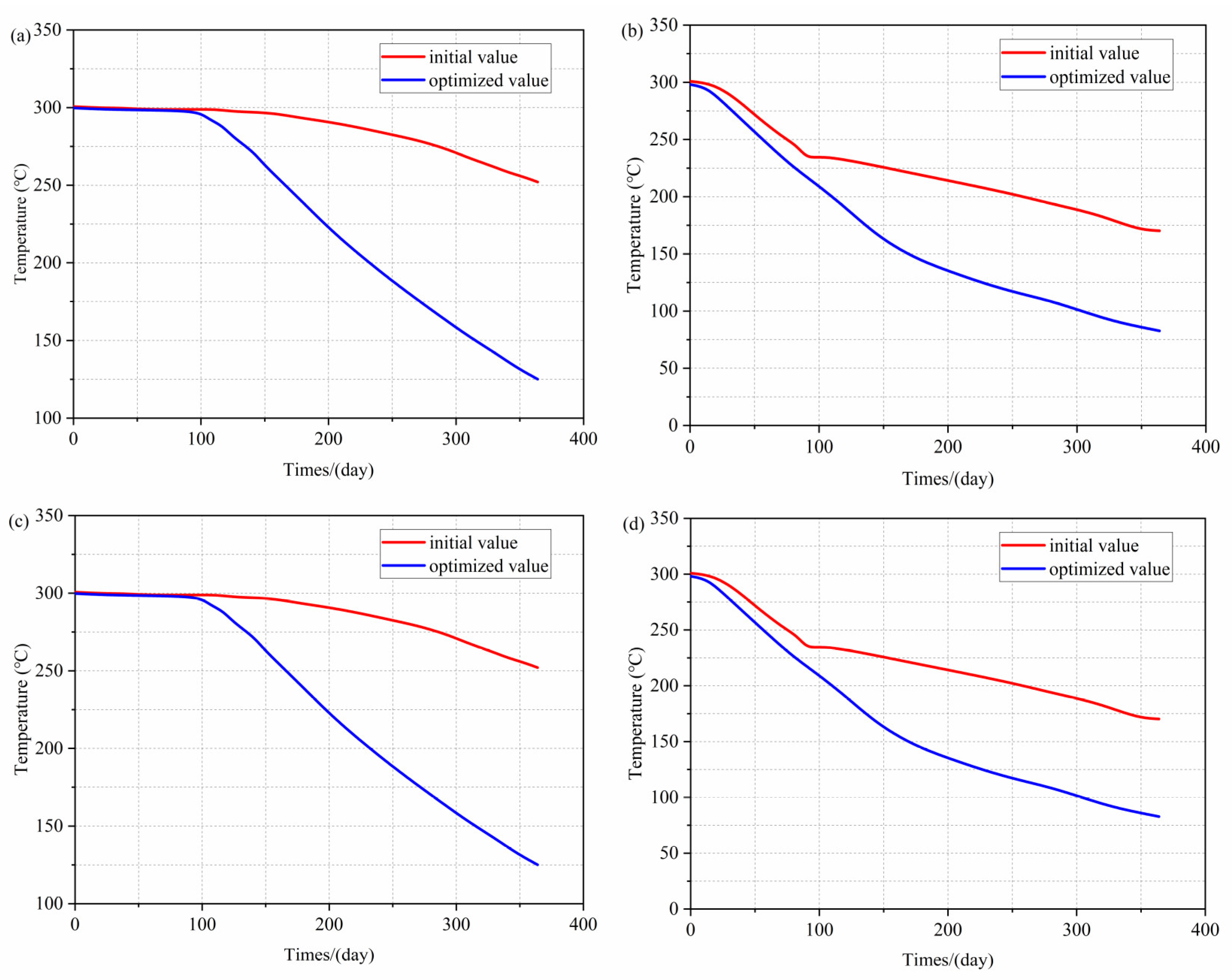
By optimizing the location and head pressure of production wells, the full use of geothermal resources and geothermal recovery can be adjusted according to the demand for electricity. According to the actual power generation application of an EGS, the net power generation is taken as the objective function, and the position and pressure of each production well are simultaneously optimized according to the difference in injection amount and injection water temperature in different seasons. The results show that after optimization, the temperature of each production well can remain above the lowest temperature required for power generation, and the power generation is also increased significantly.

References

1. Willems, C.J.L.; Nick, H.M. Towards optimisation of geothermal heat recovery: An example from the West Netherlands Basin. Appl. Energy 2019, 247, 582–593. [Google Scholar] [CrossRef]
2. Zhao, Y.; Feng, Z.; Feng, Z.; Yang, D.; Liang, W. THM (Thermo-hydro-mechanical) coupled mathematical model of fractured media and numerical simulation of a 3D enhanced geothermal system at 573 K and buried depth 6000–7000 M. Energy 2015, 82, 193–205. [Google Scholar] [CrossRef]
3. Gan, Q.; Elsworth, D. Production optimization in fractured geothermal reservoirs by coupled discrete fracture network modeling. Geothermics 2016, 62, 131–142. [Google Scholar] [CrossRef] [Green Version]
4. Shaik, A.R.; Rahman, S.S.; Tran, N.H.; Tran, T. Numerical simulation of Fluid-Rock coupling heat transfer in naturally fractured geothermal system. Appl. Therm. Eng. 2011, 31, 1600–1606. [Google Scholar] [CrossRef]
5. Li, S.; Feng, X.-T.; Zhang, D.; Tang, H. Coupled thermo-hydro-mechanical analysis of stimulation and production for fractured geothermal reservoirs. Appl. Energy 2019, 247, 40–59. [Google Scholar] [CrossRef]
6. Wang, W.X.; Sui, W.H.; Faybishenko, B.; Stringfellow, W.T. Permeability variations within mining-induced fractured rock mass and its influence on groundwater inrush. Environ. Earth Sci. 2016, 75, 326. [Google Scholar] [CrossRef] [Green Version]
7. Zhang, S.; Fan, G.; Zhang, D.; Li, S.; Chen, M.; Fan, Y.; Luo, T. Impacts of longwall mining speeds on permeability of weakly cemented strata and subsurface watertable: A case study. Geomat. Nat. Hazards Risk 2021, 12, 3063–3088. [Google Scholar] [CrossRef]
8. Liu, X.; Liu, Q.; Liu, B.; Kang, Y.; He, J. Numerical manifold method for thermal–hydraulic coupling in fractured enhance geothermal system. Eng. Anal. Bound. Elem. 2019, 101, 67–75. [Google Scholar] [CrossRef]
9. Zhang, L.; Jiang, P.; Wang, Z.; Xu, R. Convective heat transfer of supercritical CO2 in a rock fracture for enhanced geothermal systems. Appl. Therm. Eng. 2017, 115, 923–936. [Google Scholar] [CrossRef]
10. Na, J.; Xu, T.; Yuan, Y.; Feng, B.; Tian, H.; Bao, X. An integrated study of fluid–rock interaction in a CO2-based enhanced geothermal system: A case study of Songliao Basin, China. Appl. Geochem. 2015, 59, 166–177. [Google Scholar] [CrossRef]
11. Faigle, B.; Elfeel, M.A.; Helmig, R.; Becker, B.; Flemisch, B.; Geiger, S. Multi-physics modeling of non-isothermal compositional flow on adaptive grids. Comput. Methods Appl. Mech. Eng. 2015, 292, 16–34. [Google Scholar] [CrossRef]
12. Xu, J.; Yang, K. Well-posedness and robust preconditioners for discretized fluid–structure interaction systems. Comput. Methods Appl. Mech. Eng. 2015, 292, 69–91. [Google Scholar] [CrossRef] [Green Version]
13. Zhang, Y.; Zhuang, X. Cracking elements: A self-propagating Strong Discontinuity embedded Approach for quasi-brittle fracture. Finite Elem. Anal. Des. 2018, 144, 84–100. [Google Scholar] [CrossRef]
14. Koh, J.; Roshan, H.; Rahman, S.S. A numerical study on the long term thermo-poroelastic effects of cold water injection into naturally fractured geothermal reservoirs. Comput. Geotech. 2011, 38, 669–682. [Google Scholar] [CrossRef]
15. Jiang, F.; Luo, L.; Chen, J. A novel three-dimensional transient model for subsurface heat exchange in enhanced geothermal systems. Int. Commun. Heat Mass Transf. 2013, 41, 57–62. [Google Scholar] [CrossRef]
16. Zeng, Y.-C.; Su, Z.; Wu, N.-Y. Numerical simulation of heat production potential from hot dry rock by water circulating through two horizontal wells at Desert Peak geothermal field. Energy 2013, 56, 92–107. [Google Scholar] [CrossRef]
17. Huang, W.; Cao, W.; Jiang, F. Heat extraction performance of EGS with heterogeneous reservoir: A numerical evaluation. Int. J. Heat Mass Transf. 2017, 108, 645–657. [Google Scholar] [CrossRef] [Green Version]
18. Huang, W.; Cao, W.; Guo, J.; Jiang, F. An analytical method to determine the fluid-rock heat transfer rate in two-equation thermal model for EGS heat reservoir. Int. J. Heat Mass Transf. 2017, 113, 1281–1290. [Google Scholar] [CrossRef]
19. Yan, C.; Jiao, Y.-Y.; Yang, S. A 2D coupled hydro-thermal model for the combined finite-discrete element method. Acta Geotech. 2018, 14, 403–416. [Google Scholar] [CrossRef]
20. Jasinski, L.; Dabrowski, M. The Effective Transmissivity of a Plane-Walled Fracture With Circular Cylindrical Obstacles. J. Geophys. Res. Solid Earth 2018, 123, 242–263. [Google Scholar] [CrossRef] [Green Version]
21. Hyman, J.D.; Aldrich, G.; Viswanathan, H.; Makedonska, N.; Karra, S. Fracture size and transmissivity correlations: Implications for transport simulations in sparse three-dimensional discrete fracture networks following a truncated power law distribution of fracture size. Water Resour. Res. 2016, 52, 6472–6489. [Google Scholar] [CrossRef]
22. Fairley, J.P. Fracture/matrix interaction in a fracture of finite extent. Water Resour. Res. 2010, 46, 1–11. [Google Scholar] [CrossRef] [Green Version]
23. Li, L.; Jiang, H.; Li, J.; Wu, K.; Meng, F.; Xu, Q.; Chen, Z. An analysis of stochastic discrete fracture networks on shale gas recovery. J. Pet. Sci. Eng. 2018, 167, 78–87. [Google Scholar] [CrossRef]
24. Lei, Q.; Latham, J.-P.; Tsang, C.-F. The use of discrete fracture networks for modelling coupled geomechanical and hydrological behaviour of fractured rocks. Comput. Geotech. 2017, 85, 151–176. [Google Scholar] [CrossRef]
25. Hyman, J.D.; Karra, S.; Makedonska, N.; Gable, C.W.; Painter, S.L.; Viswanathan, H.S. dfnWorks: A discrete fracture network framework for modeling subsurface flow and transport. Comput. Geosci. 2015, 84, 10–19. [Google Scholar] [CrossRef] [Green Version]
26. Figueiredo, B.; Tsang, C.-F.; Rutqvist, J.; Niemi, A. A study of changes in deep fractured rock permeability due to coupled hydro-mechanical effects. Int. J. Rock Mech. Min. Sci. 2015, 79, 70–85. [Google Scholar] [CrossRef] [Green Version]
27. Akın, S.; Kok, M.V.; Uraz, I. Optimization of well placement geothermal reservoirs using artificial intelligence. Comput. Geosci. 2010, 36, 776–785. [Google Scholar] [CrossRef]
28. Chen, J.; Jiang, F. Designing multi-well layout for enhanced geothermal system to better exploit hot dry rock geothermal energy. Renew. Energy 2015, 74, 37–48. [Google Scholar] [CrossRef]
29. Zeng, Y.-C.; Wu, N.-Y.; Su, Z.; Wang, X.-X.; Hu, J. Numerical simulation of heat production potential from hot dry rock by water circulating through a novel single vertical fracture at Desert Peak geothermal field. Energy 2013, 63, 268–282. [Google Scholar] [CrossRef]
30. Duniam, S.; Gurgenci, H. Annual performance variation of an EGS power plant using an ORC with NDDCT cooling. Appl. Therm. Eng. 2016, 105, 1021–1029. [Google Scholar] [CrossRef] [Green Version]
31. Xu, T.; Yuan, Y.; Jia, X.; Lei, Y.; Li, S.; Feng, B.; Hou, Z.; Jiang, Z. Prospects of power generation from an enhanced geothermal system by water circulation through two horizontal wells: A case study in the Gonghe Basin, Qinghai Province, China. Energy 2018, 148, 196–207. [Google Scholar] [CrossRef]
32. Meng, N.; Li, T.; Wang, J.; Jia, Y.; Liu, Q.; Qin, H. Synergetic mechanism of fracture properties and system configuration on techno-economic performance of enhanced geothermal system for power generation during life cycle. Renew. Energy 2020, 152, 910–924. [Google Scholar] [CrossRef]
33. Patil, V.R.; Biradar, V.I.; Shreyas, R.; Garg, P.; Orosz, M.S.; Thirumalai, N.C. Techno-economic comparison of solar organic Rankine cycle (ORC) and photovoltaic (PV) systems with energy storage. Renew. Energy 2017, 113, 1250–1260. [Google Scholar] [CrossRef]
34. Zimmerman, R.W.; Bodvarsson, G.S. Hydraulic conductivity of rock fractures. Transp. Porous Media 1996, 23, 1–30. [Google Scholar] [CrossRef] [Green Version]
35. Ghassemi, A.; Zhou, X. A three-dimensional thermo-poroelastic model for fracture response to injection/extraction in enhanced geothermal systems. Geothermics 2011, 40, 39–49. [Google Scholar] [CrossRef]
36. Gao, Y.; Guo, P.; Zhang, Z.; Li, M.; Gao, F.; Wang, Y. Migration of the Industrial Wastewater in Fractured Rock Masses Based on the Thermal-Hydraulic-Mechanical Coupled Model. Geofluids 2021, 2021, 5473719. [Google Scholar] [CrossRef]
37. Bohnsack, D.; Potten, M.; Pfrang, D.; Wolpert, P.; Zosseder, K. Porosity–permeability relationship derived from Upper Jurassic carbonate rock cores to assess the regional hydraulic matrix properties of the Malm reservoir in the South German Molasse Basin. Geotherm. Energy 2020, 8, 12. [Google Scholar] [CrossRef] [Green Version]
38. Júnior, V.A.S.; Júnior, A.F.S.; Simões, T.A.; Oliveira, G.P. Poiseuille-Number-Based Kozeny–Carman Model for Computation of Pore Shape Factors on Arbitrary Cross Sections. Transp. Porous Media 2021, 138, 99–131. [Google Scholar] [CrossRef]
39. Rutqvist, J.; Wu, Y.-S.; Tsang, C.-F.; Bodvarsson, G. A modeling approach for analysis of coupled multiphase fluid flow, heat transfer, anddeformation in fracturedporous rock. Int. J. Rock Mech. Min. Sci. 2002, 39, 11. [Google Scholar] [CrossRef]
40. Min, K.-B.; Rutqvist, J.; Elsworth, D. Chemically and mechanically mediated influences on the transport and mechanical characteristics of rock fractures. Int. J. Rock Mech. Min. Sci. 2009, 46, 80–89. [Google Scholar] [CrossRef] [Green Version]
41. Brown, S.R.; Scholz, C.H. Closure of rock joints. J. Geophys. Res. 1986, 91, 4939–4948. [Google Scholar] [CrossRef]
42. Baldino, S.; Meng, M. Critical review of wellbore ballooning and breathing literature. Geomech. Energy Environ. 2021, 28, 100252. [Google Scholar] [CrossRef]
43. Chen, Y.; Ma, G.; Wang, H.; Li, T. Evaluation of geothermal development in fractured hot dry rock based on three dimensional unified pipe-network method. Appl. Therm. Eng. 2018, 136, 219–228. [Google Scholar] [CrossRef]
44. Mahmoodpour, S.; Singh, M.; Bär, K.; Sass, I. Thermo-hydro-mechanical modeling of an enhanced geothermal system in a fractured reservoir using carbon dioxide as heat transmission fluid—A sensitivity investigation. Energy 2022, 254, 124266. [Google Scholar] [CrossRef]
45. Mahmoodpour, S.; Singh, M.; Turan, A.; Bär, K.; Sass, I. Simulations and global sensitivity analysis of the thermo-hydraulic-mechanical processes in a fractured geothermal reservoir. Energy 2022, 247, 123511. [Google Scholar] [CrossRef]
46. Mahmoodpour, S.; Singh, M.; Bär, K.; Sass, I. Impact of Well Placement in the Fractured Geothermal Reservoirs Based on Available Discrete Fractured System. Geosciences 2022, 12, 19. [Google Scholar] [CrossRef]
47. Mahmoodpour, S.; Singh, M.; Turan, A.; Bär, K.; Sass, I. Hydro-Thermal Modeling for Geothermal Energy Extraction from Soultz-sous-Forêts, France. Geosciences 2021, 11, 464. [Google Scholar] [CrossRef]
Figure 1. Schematic of the geothermal recovery system before and after geometric simplification.
Sustainability 15 09744 g001
Figure 2. Meshing of simplified and unreduced models: (a) simplified model, 31,274 mesh elements; (b) unreduced model, 15,750,953 mesh elements.
Sustainability 15 09744 g002
Figure 3. Temperature distribution along the direction of the line connecting two wellbores.
Sustainability 15 09744 g003
Figure 4. (a) Discrete fracture network in the thermal reservoir model; (b) tetrahedral mesh used for the thermal simulation.
Sustainability 15 09744 g004
Figure 5. Simulation results for a production period of 10 years: (a) average outlet temperatures; (b) average reservoir temperatures; (c) reservoir power generations; (d) average fracture apertures.
Sustainability 15 09744 g005
Figure 6. Injection well conditions: (a) Relationship between normal injection velocity and time; (b) Relationship between injection water temperature and time.
Sustainability 15 09744 g006
Figure 7. Improvement results for power generation efficiency optimization over the course of 80 days.
Sustainability 15 09744 g007
Figure 8. Temperature distribution of the reservoir: (a) position and pressure of each production well are not optimized; (b) position and pressure of each production well are optimized.
Sustainability 15 09744 g008
Figure 9. The evolution of fluid velocity in terms of time of each production well: (a) well 1; (b) well 2; (c) well 3; (d) well 4.
Sustainability 15 09744 g009
Figure 10. The evolution of temperature of fluid in terms of time of each production well: (a) well 1; (b) well 2; (c) well 3; (d) well 4.
Sustainability 15 09744 g010