
Analysis of Efficiency Differences and Research on Moderate Operational Scale of New Agricultural Business Entities in Northeast China

Abstract
1. Introduction
2. Problem Descriptions and Research Methods
2.1. Problem Descriptions and Analysis
2.1.1. Efficiency Differences
2.1.2. Moderate Business Scale
2.2. Research Methodology
2.2.1. Research Methods for Analyzing Differences in The Efficiency of Business Entities
2.2.2. Research Methods for Moderate Business Scale of Best Business Entities
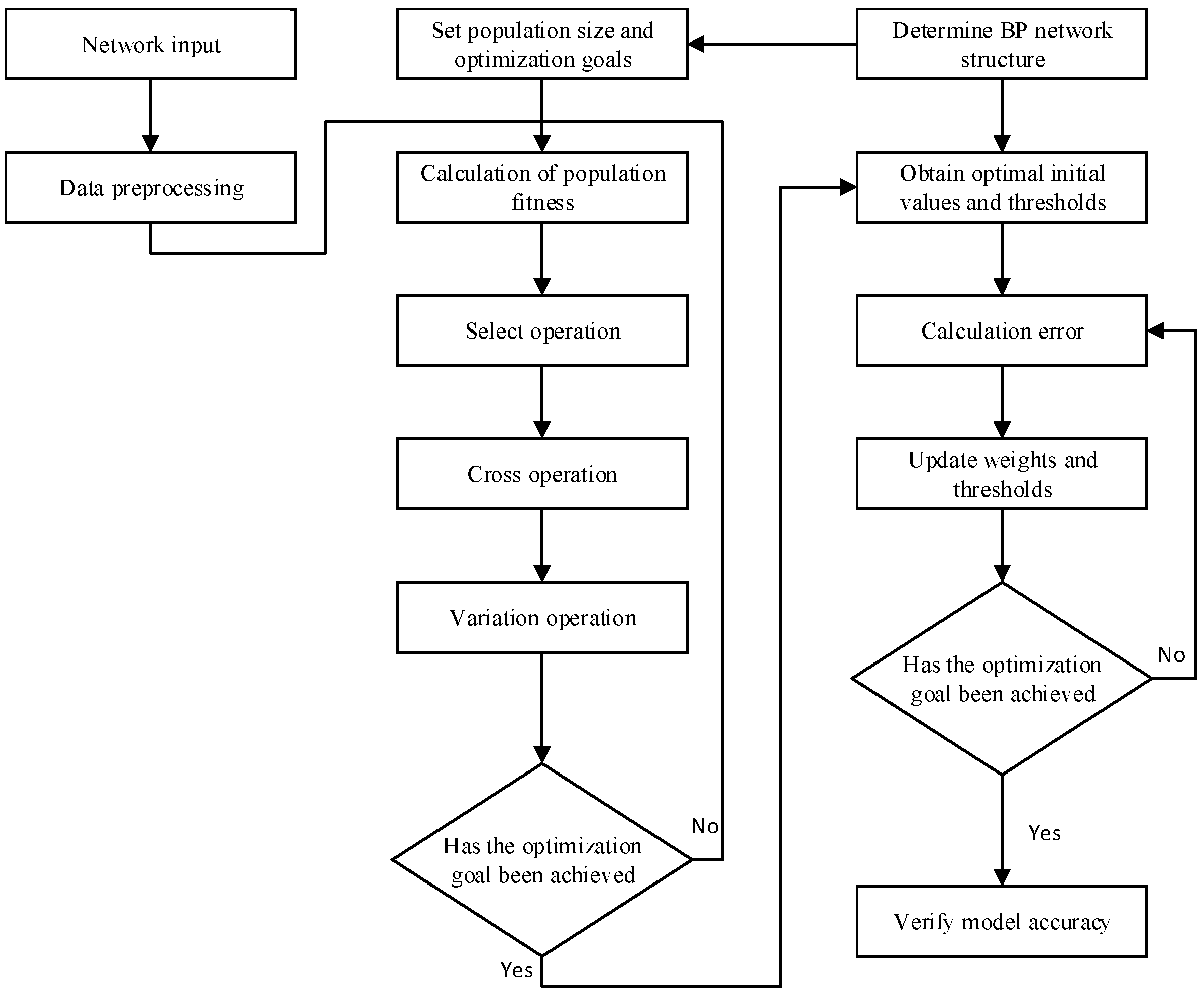
- DEA-GA-BP neural network prediction model
- 2.
- Entropy method-grey correlation analysis method
3. Indicator Descriptions and Data Acquisition
3.1. Description of Indicators
3.2. Data Acquisition
4. Results and Analysis
4.1. Efficiency Calculation Results and Analysis of Agricultural Business Entities
4.1.1. Results of DEA-BCC Model Calculation
4.1.2. Results of Cross-Efficiency DEA Model
4.1.3. Analysis and Discussion of Efficiency Calculation Results
- Comparing the average values of comprehensive technical efficiency, pure technical efficiency, and scale efficiency of the agricultural business entities.
- 2.
- Compare the average cross-efficiency values of the agricultural business entities.
- 3.
- Comparison of efficiency values for different types of agricultural business entities under two models.
4.2. Forecast and Analyse the Moderation of Business Scale of Family Farm
4.2.1. Results of DEA-GA-BP Prediction Model
- Network structure and parameters
- 2.
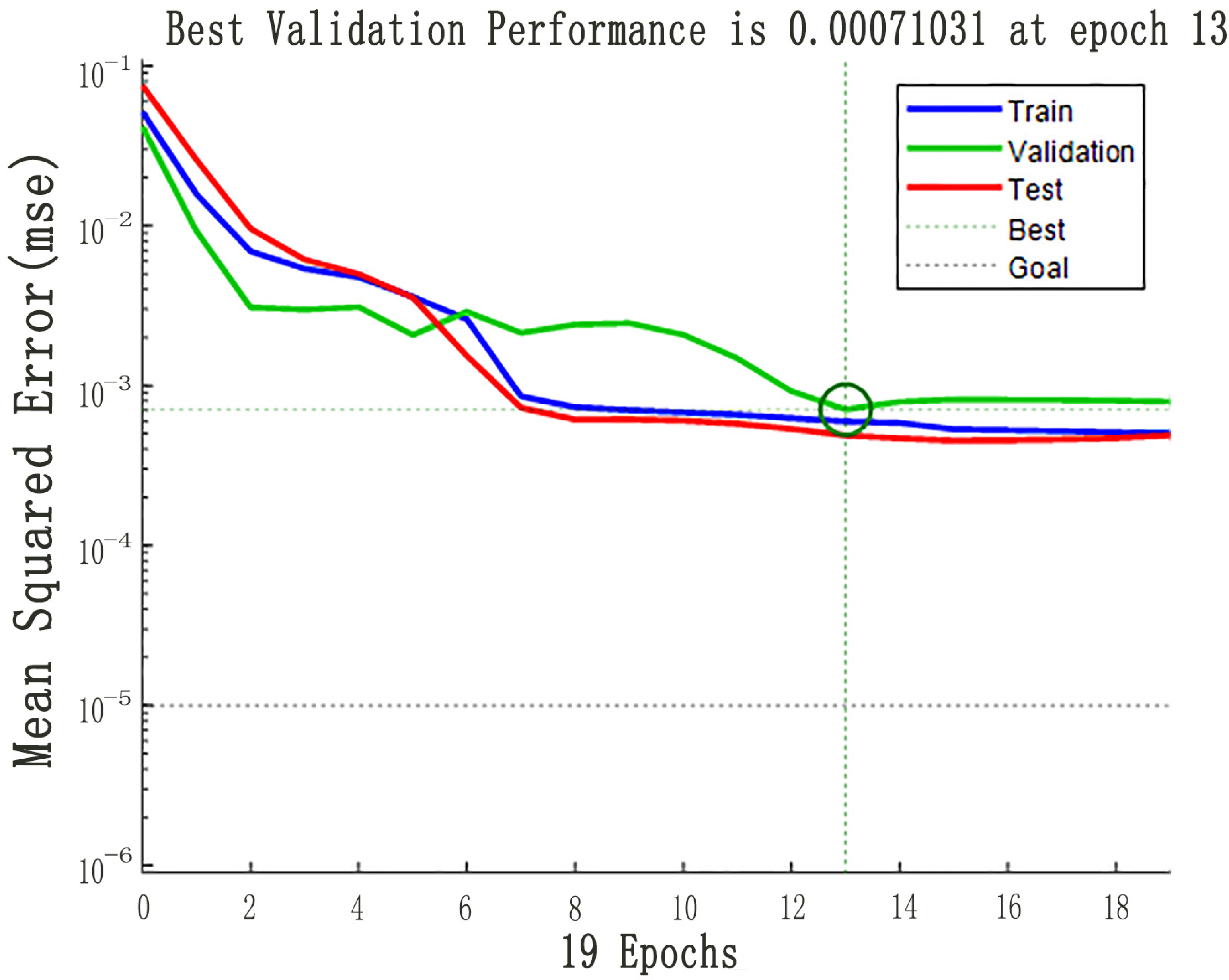
- Fitting effect
- Prediction accuracy
4.2.2. Results of Moderate Operational Scale of Family Farm Based on Entropy Method and Grey Relational Analysis Method
4.2.3. Analysis and Discussion of Results on The Appropriateness of Business Scale
- The DEA-GA-BP prediction model can be further optimized.
- 2.
- The optimal scale of operation can be further analyzed.
5. Discussion
- Discussion on the analysis of efficiency differences among new agricultural business entities.
- 2.
- Discussion on the moderate operational scale of new agricultural business entities.
6. Conclusions and Suggestions
6.1. Conclusions
- The DEA-BCC model and the cross-efficiency DEA model were used to measure and calculate the efficiency of different agricultural business entities, and the comprehensive analysis of the results of the two models showed that the most suitable type of agriculture for dry farmland crops in Northeast China was the family farm.
- The DEA-GA-BP prediction model had higher goodness of fit and a smaller relative error than the ordinary BP-ANN model, which verified the effectiveness of the DEA-GA-BP prediction model proposed in this paper.
- The entropy method and gray relational analysis method were used to calculate the value of the correlation degree of the scheme combination of family farms. The optimal management combination for a family farm for dry farmland crops in Northeast China was obtained as follows: when the range of input for farmland planting area is 9015 to 10,000 mu, the range of direct input is 6,160,060 RMB to 6,840,500 RMB; the range of indirect input is 733,008 RMB to 1,213,400 RMB; the range of artificial input is 51,200 RMB to 100,000 RMB; and the range of mechanical input is 22,800 RMB to 1,100,000 RMB. At this time, the range of maximum output value is 12,347,630 RMB to 12,349,290 RMB; the total net income is 5,910,000 RMB.
6.2. Measures and Suggestions
- The construction of new agricultural business entities should focus on the development of family farms.
- 2.
- Optimize the allocation ratio of production factors in family farms.
- 3.
- Strengthen the effective application of advanced production technology on family farms.
Author Contributions
Funding
Institutional Review Board Statement
Informed Consent Statement
Data Availability Statement
Acknowledgments
Conflicts of Interest
References
- Kimhi, A. Plot size and maize productivity in Zambia: Is there an inverse relationship? J. Agric. Econ. 2006, 35, 1–9. [Google Scholar] [CrossRef]
- Helfand, S.M.; Levine, E.S. Farm Size and the Determinants of Productivity Efficiency in the Brazilian Center-West. J. Agric. Econ. 2004, 31, 241–249. [Google Scholar] [CrossRef]
- Zhou, M.; Huang, S.L.; Zhang, Y.; Lin, J. Moderate scale of agricultural land management and its restraining factor in Heilongjiang province. J. Arid Land Resour. Environ. 2018, 32, 37–41. [Google Scholar]
- Han, J.; Liu, S.Y.; Zhang, S.F. Influence of aging of agricultural labor force on large-scale management of land. J. Resour. Sci. 2019, 41, 2284–2295. [Google Scholar] [CrossRef]
- Wang, Y.H.; Li, X.B.; Xin, L.J. The impact of farm land management scale on agricultural labor productivity in China and its regional differentiation. J. Nat. Resour. 2017, 32, 539–552. [Google Scholar]
- Giang, L.T.; Nguyen, K.M. Efficiency Estimates for the Agricultural Production in Vietnam: A Comparison of Parametric and Non-parametric Approaches. J. Agric. Econ. Rev. 2010, 10, 62–78. [Google Scholar]
- Marvin, H.J.P.; Kleter, G.A. Proactive systems for early warning of potential impacts of natural disasters on food safety: Climate-change-induced extreme events as case in point. J. Food Control 2013, 34, 444–456. [Google Scholar] [CrossRef]
- Lunik, E.; Langemeier, M. International Comparison of Cost and Efficiency of Corn and Soybean Production. In Proceedings of the 2015 Annual Meeting, Southern Agricultural Economics Association, Atlanta, GA, USA, 31 January–3 February 2015. [Google Scholar]
- Ma, Y.C.; Guo, X.W. Analysis of Agricultural Production Efficiency in Liaoning Province Based on Three-Stage DEA Model. J. Agric. Econ. 2019, 384, 15–17. [Google Scholar]
- Adhikari, C.B. Analyses of technical efficiency using SDF and DEA models: Evidence from Nepalese agriculture. J. Appl. Econ. 2012, 44, 3297–3308. [Google Scholar] [CrossRef]
- Xiao, S.L.; Zhu, X.Y. Analysis of total factor productivity of grain production of Henan Province based on SFA. J. Henan Agric. Univ. 2015, 49, 861–865. [Google Scholar]
- Dong, Y. Research on China’s Agricultural Technical Progress from the Perspective of Total Factor Productivity and Its Spillover Effects. Ph.D. Thesis, China Agricultural University, Beijing, China, 2016. [Google Scholar]
- Chen, Y.Q.; Wang, H.R. Evaluation of agricultural production efficiency and study on its influential factors in Jiang-Xi province. J. East China Econ. Manag. 2016, 30, 21–28. [Google Scholar]
- Xia, Z.Z. Re-recognition of agricultural moderate scale operation based on “middle farmers’ family farms”. J. Shanxi Agric. Univ. (Soc. Sci. Ed.) 2019, 18, 3–9. [Google Scholar]
- Ahamd, M.; Chaudhry, G.M.; Iqbal, M. Wheat productivity efficiency and sustainability: A stochastic production frontier analysis. J. Pak. Dev. Rev. 2002, 41, 643–663. [Google Scholar] [CrossRef]
- Renato, V.; Euan, F. Technical inefficiency, and production risk in rice farming: Evidence from Central Luzon Philippines. J. Asian Econ. J. 2006, 20, 29–46. [Google Scholar]
- Fan, S.; Chan-Kang, C. Is small beautiful? Farm size, productivity, and poverty in Asian agriculture. J. Agric. Econ. 2005, 32, 135–146. [Google Scholar] [CrossRef]
- Varga, T. Potential for efficiency improvement of Hungarian agriculture. J. Stud. Agric. Econ. 2006, 104, 85–107. [Google Scholar]
- Liu, Y. Impacts of Farmland Transfer on Agricultural Production and Farmers’ Income: An Empirical Study in Gansu Province. Ph.D. Thesis, Lanzhou University, Lanzhou, China, 2018. [Google Scholar]
- Kong, L.C.; Zheng, S. Research on operating efficiency and moderate scale of family farm—Based on DEA model’s analysis of Song-Jiang model. J. Northwest AF Univ. (Soc. Sci. Ed.) 2016, 16, 107–118. [Google Scholar]
- Dong, S. Study on Moderate Scale Management of Grain Production Family Farm in Chang-Chun City. Master’s Thesis, Jilin University, Changchun, China, 2020. [Google Scholar]
- Wei, R. Study on the Moderate Scale Operation of Grain Production Based on the Agricultural Management Entities—Taking the Huang-Huai-Hai Region as an Example. Ph.D. Thesis, Chinese Academy of Agricultural Sciences, Beijing, China, 2016. [Google Scholar]
- Sun, R. Research on the Rural-Household Differentiation and Moderate Scale Agricultural Development in Beijing-Tianjin. Ph.D. Thesis, Tianjin University of Finance and Economics, Tianjin, China, 2017. [Google Scholar]
- Chen, Y.F.; Feng, Z.C. Impact of moderate and scale operation to the International competitiveness of rape planning: An evidence from 360 houses in Hubei Province. J. China Agric. Univ. 2019, 24, 190–200. [Google Scholar]
- Fan, S.; Qi, J.L. A Study on the Supply and Demand of Rural Labor Force from the Perspective of Moderate Land Scale Management: A Case Study of Shenyang City. J. Contemp. Econ. 2019, 500, 110–112. [Google Scholar]
- Xu, Y.; Xin, L.; Li, X.; Tan, M.; Wang, Y. Exploring a Moderate Operation Scale in China’s Grain Production: A Perspective on the Costs of Machinery Services. Sustainability 2019, 11, 2213. [Google Scholar] [CrossRef]
- Sun, X.B. Research on Operating Efficiency of Guangzhou Port Company Based on Two-Stage DEA Model. Master’s Thesis, South China University of Technology, Guangzhou, China, 2019. [Google Scholar]
- Zhong, Y. Cross Efficiency Evaluation Based on the Importance of Output. Master’s Thesis, East China Jiao-Tong University, Nanchang, China, 2016. [Google Scholar]
- Liu, H.R.; Zhao, C.X. Study on a neural network optimization algorithm based on improved genetic algorithm. J. Sci. Instrum. 2016, 37, 1573–1580. [Google Scholar]
- Qin, G.H.; Xie, W.B. Detection and control for tool wear based Online network and genetic algorithm. J. Opt. Precis. Eng. 2015, 23, 1314–1321. [Google Scholar]
- Zhang, D.; Cheney, J.J. Evaluation System for College Counselors Based on Entropy Method and Grey Correlation Method. J. Contemp. Educ. Pract. Teach. Res. 2019, 13, 138–140. [Google Scholar]
- Li, W.Q. Research on Comprehensive Evaluation of Rationality of Tax Burden in China—Based on Entropy Grey Relational Analysis. Master’s Thesis, Shandong University, Jinan, China, 2019. [Google Scholar]
- Wang, L.J. Empirical Study on the High-Quality Development Level of Manufacturing Industry in Liaoning Province—Gray Correlation Analysis Based on Entropy Method. Master’s Thesis, Liaoning University, Shenyang, China, 2019. [Google Scholar]
- Chavas, J.P.; Roth, P.M. Farm Household Production Efficiency: Evidence from the Gambia. J. Am. J. Agric. Econ. 2005, 87, 160–179. [Google Scholar] [CrossRef]
- Zheng, T.W.; Zhang, Y.J. Study on the Management Efficiency and Scale of Corn Family Farms in Jilin Province. J. Maize Sci. 2022, 30, 185–190. [Google Scholar]
- He, T.T. Dynamic Changes and Factors of Growth of Agricultural Total Factor Productivity in China—Based on a Compare Study by Using DEA and SFA. J. Chongqing Univ. Arts Sci. (Soc. Sci. Ed.) 2017, 36, L3-21.4. [Google Scholar]
- Mehta, C.R.; Chandel, N.S. Status, Challenges and Strategies for Farm Mechanization in India. J. AMA Agric. Mech. Asia Afr. Lat. Am. 2014, 45, 43–50. [Google Scholar]
- Tong, G.J.; Li, W.F. Comparative Study on the Production Efficiency of New Agricultural Management Entities—Taking Maize Planting Management Entities in Four Provinces as an Example. J. Dong Yue Tribune 2022, 43, 140–147. [Google Scholar]
- Wu, F. Measurement of Technical Efficiency and Analysis of Influencing Factors of Family Farm Based on SFA. J. Hua-Zhong Agric. Univ. (Soc. Sci. Ed.) 2020, 48–56+162–163. [Google Scholar]
- Niu, H.; Chen, S.W.; An, K. Does Agricultural Insurance Meet the Protection Needs of New Agricultural Operators—Evidence Based on 422 Provincial Demonstration Family Farms in Shandong Province. J. Insur. Stud. 2020, 386, 58–68. [Google Scholar]
- Gu, R.P.; Lai, J.H. Prediction Method of Flight delay based on Grey GA-BP neural Network. J. Comput. Integr. Manuf. Syst. 2022, 39, 38–43+59. [Google Scholar]
- Kazimipour, B.; Li, X.; Qin, K. A review of population initialization techniques for evolutionary algorithms. In Proceedings of the 2014 IEEE Congress on Evolutionary Computation (CEC), Beijing, China, 6–11 July 2014. [Google Scholar]
- Yang, Y.Q. Parameters optimization of polygonal fuzzy neural networks based on GA-BP hybrid algorithm. Int. J. Mach. Learn. Cybern. 2014, 5, 815–822. [Google Scholar] [CrossRef]
- Zhan, X.; He, N. Study on Classification and Applicability of Comprehensive Evaluation Methods. J. Stat. Decis. 2022, 38, 31–36. [Google Scholar]
- Zhu, J.D. A Comparative Study on Production Efficiency of New Agricultural Production and Management Entities—Based on the survey data of Xinyang City. J. Chin. J. Agric. Resour. Reg. Plan. 2017, 38, 181–189. [Google Scholar]
- Xu, J.B.; Wang, Y. Is new agricultural management entity capable of promoting the development of small holders: From the perspective of technical efficiency comparison. J. China Agric. Univ. 2020, 25, 200–214. [Google Scholar]
- Lowder, S.K.; Skoet, J. The Number, Size, and Distribution of Farms, Smallholder Farms, and Family Farms Worldwide. World Dev. 2016, 87, 16–29. [Google Scholar] [CrossRef]
- Guan, F.X. The Land Scale of Grain Production Family Farms in North China Plain: An Example from Henan, a Major Grain Production Province. J. Chin. Rural. Econ. 2018, 22–38. [Google Scholar]
- Yan, X.; Wang, Y.; Yang, G.; Liao, N.; Li, F. Research on the Scale of Agricultural Land Moderate Management and Countermeasures Based on Farm Household Analysis. Sustainability 2021, 13, 10591. [Google Scholar] [CrossRef]
- Shi, Y.; Yang, Q.; Zhou, L.; Shi, S. Can Moderate Agricultural Scale Operations Be Developed against the Background of Plot Fragmentation and Land Dispersion? Evidence from the Suburbs of Shanghai. Sustainability 2022, 14, 8697. [Google Scholar] [CrossRef]


| Type of Indicator | Selection of Indicators | Unit of Measurement | Indicator Description |
|---|---|---|---|
| Input indicators | Direct input | Yuan | Including other direct costs such as seeds, fertilizers, farmyard manure, pesticides, farmland transfer fees, drainage and irrigation, animal power, technical services, tools and materials, repairs and maintenance |
| Indirect input | Yuan | Including depreciation of fixed assets, insurance, management fees, finance costs, selling fees, depreciation of rent for own camp, etc. | |
| Labor input | Yuan | Including the amount of labor employed and the discounted price for domestic labor | |
| Farmland input | Acres | Total area of farmland operated by agricultural business entities | |
| Mechanical input | Yuan | Includes the value of agricultural machinery and machinery operations, fuel and power costs, machinery repair and maintenance costs, agricultural mechanics’ hiring costs and other machinery-related costs | |
| Output indicators | Total net income | Yuan | Annual net income of the operating entity, including the government subsidy component and net income from farming operations |
| Output value | Yuan | Annual income of the operating entity |
| Sample Business Entities | Number of Samples | Average Farmland Input (Acres) | Average Direct Input (Yuan) | Average Indirect Input (Yuan) | Average Labor Input (Yuan) | Average Machinery Input (Yuan) | Average Output Value (Yuan) | Average Net Income (Yuan) |
|---|---|---|---|---|---|---|---|---|
| Farmers | 20 | 86 | 14,673 | 6538 | 14,000 | 15,879 | 71,895 | 20,800 |
| Family farms | 56 | 1761.8036 | 883,570 | 134,831 | 33,175 | 178,095 | 1,697,064 | 467,392 |
| Large professional households | 14 | 482.5000 | 218,661 | 57,006 | 18,293 | 94,643 | 536,222 | 147,620 |
| Agricultural Cooperative | 16 | 3988.6875 | 2,709,178 | 546,027 | 376,363 | 267,477 | 5,228,556 | 1,329,512 |
| Type | Number | Scale Area (Acres) | Input Indicators | Output Indicators | |||||
|---|---|---|---|---|---|---|---|---|---|
| Direct Input (Yuan) | Indirect Input (Yuan) | Labor Input (Yuan) | Farmland Input (Acres) | Machinery Input (Yuan) | Output Value (Yuan) | Total Net Income (Yuan) | |||
| Largerurual Professional households | 1 | <200 | 66,500 | 58,650 | 19,560 | 150.000 | 18,200 | 183,750 | 24,800 |
| 2 | 200 ≤ s < 500 | 177,230 | 27,650 | 23,310 | 299.125 | 45,690 | 369,490 | 85,610 | |
| 3 | 500 ≤ s < 1000 | 303,920 | 35,920 | 27,330 | 517.333 | 89,970 | 495,400 | 138,260 | |
| 4 | 1000 ≤ s < 2000 | 492,560 | 205,240 | 58,800 | 1330.000 | 305,700 | 1,360,600 | 298,300 | |
| Agriculture cooperative | 5 | 500 ≤ s < 1000 | 255,670 | 223,760 | 147,500 | 700.000 | 95,910 | 964,380 | 241,540 |
| 6 | 1000 ≤ s < 2000 | 562,420 | 292,420 | 248,750 | 1488.750 | 322,910 | 1,673,440 | 386,940 | |
| 7 | 2000 ≤ s < 1000 | 2,492,830 | 308,360 | 507,980 | 5073.778 | 399,570 | 5,228,490 | 2,019,760 | |
| 8 | ≥10,000 | 5,950,400 | 644,000 | 700,000 | 10,800.00 | 520,040 | 11,758,000 | 4,243,560 | |
| Family farm | 9 | <200 | 47,100 | 38,200 | 12,650 | 150.000 | 48,650 | 187,550 | 42,150 |
| 10 | 200 ≤ s < 500 | 135,250 | 43,710 | 41,760 | 334.455 | 45,510 | 408,820 | 132,590 | |
| 11 | 500 ≤ s < 1000 | 293,050 | 80,430 | 41,690 | 650.667 | 91,190 | 705,340 | 218,980 | |
| 12 | 1000 ≤ s < 2000 | 603,330 | 137,290 | 52,460 | 1283.846 | 177,220 | 1,331,820 | 361,520 | |
| 13 | 2000 ≤ s < 10,000 | 2,140,170 | 221,740 | 48,000 | 4220.909 | 379,150 | 3,356,050 | 566,990 | |
| 14 | ≥10,000 | 5,422,750 | 669,730 | 159,000 | 10,000.00 | 654,330 | 12,344,200 | 5,438,380 | |
| Peasant household | 15 | 86 | 34,673 | 6538 | 40,000 | 86.000 | 5879 | 71,895 | 20,800 |
| Decision-Making Unit | Overall Technical Efficiency | Pure Technical Efficiency | Scale Efficiency | Scale Elasticity |
|---|---|---|---|---|
| DMU1 | 0.929 | 1.000 | 0.929 | Increasing |
| DMU2 | 0.989 | 1.000 | 0.989 | Increasing |
| DMU3 | 0.775 | 0.825 | 0.939 | Increasing |
| DMU4 | 0.947 | 1.000 | 0.947 | Decreasing |
| DMU5 | 1.000 | 1.000 | 1.000 | - |
| DMU6 | 0.891 | 1.000 | 0.891 | Decreasing |
| DMU7 | 0.921 | 0.925 | 0.996 | Increasing |
| DMU8 | 1.000 | 1.000 | 1.000 | - |
| DMU9 | 1.000 | 1.000 | 1.000 | - |
| DMU10 | 1.000 | 1.000 | 1.000 | - |
| DMU11 | 0.884 | 0.898 | 0.984 | Decreasing |
| DMU12 | 0.862 | 0.880 | 0.980 | Decreasing |
| DMU13 | 0.901 | 0.947 | 0.950 | Increasing |
| DMU14 | 1.000 | 1.000 | 1.000 | - |
| DMU15 | 0.840 | 1.000 | 0.840 | Increasing |
| Average value | 0.929 | 0.965 | 0.963 |
| Various Agricultural Business Entities | Comprehensive Technical Efficiency Value | Pure Technical Efficiency | Scale Efficiency |
|---|---|---|---|
| Large rural professional households | 0.907 | 0.955 | 0.949 |
| Agriculture cooperative | 0.953 | 0.981 | 0.972 |
| Family farm | 0.941 | 0.954 | 0.986 |
| Traditional household farmer | 0.840 | 1.000 | 0.840 |
| Mean value | 0.910 | 0.973 | 0.937 |
| Different Types of Agricultural Business Entities | Average Cross-Efficiency Values |
|---|---|
| Large rural professional households | 0.610 |
| Agriculture cooperative | 0.684 |
| Family farm | 0.724 |
| Traditional farmers. | 0.619 |
| Different Types of Agricultural Business Entities | DEA-BCC Efficiency Values | Cross-Over Efficiency DEA Efficiency Values |
|---|---|---|
| Large rural professional households | 0.907 | 0.610 |
| Agriculture cooperative | 0.953 | 0.684 |
| Family farms | 0.941 | 0.724 |
| Traditional farmers | 0.840 | 0.619 |
| Mean value | 0.910 | 0.610 |
| Parameters | Population Size | Crossover Probability | Mutation Probability | Maximum Iterations | Learning Rate |
|---|---|---|---|---|---|
| value | 70 | 0.3 | 0.15 | 200 | 0.01 |
| Index | Direct Input | Indirect Input | Artificial Input | Farmland Input | Mechanical Input | Output Value | Total Net Income |
|---|---|---|---|---|---|---|---|
| Weight | 0.0188 | 0.0141 | 0.0150 | 0.0290 | 0.0140 | 0.5191 | 0.3900 |
| Index | Direct Input | Indirect Input | Artificial Input | Farmland Input | Mechanical Input | Output Value | Total Net Income |
|---|---|---|---|---|---|---|---|
| Minimum Value | 6,160,060 | 733,008 | 51,200 | 9015 | 22,800 | 12,347,630 | 5,910,000 |
| Maximum Value | 6,840,500 | 1,213,400 | 100,000 | 10,000 | 1,100,000 | 12,349,290 |
Disclaimer/Publisher’s Note: The statements, opinions and data contained in all publications are solely those of the individual author(s) and contributor(s) and not of MDPI and/or the editor(s). MDPI and/or the editor(s) disclaim responsibility for any injury to people or property resulting from any ideas, methods, instructions or products referred to in the content. |
© 2023 by the authors. Licensee MDPI, Basel, Switzerland. This article is an open access article distributed under the terms and conditions of the Creative Commons Attribution (CC BY) license (https://creativecommons.org/licenses/by/4.0/).
Share and Cite
Ma, L.; Li, C.; Xin, M.; Sun, N.; Teng, Y. Analysis of Efficiency Differences and Research on Moderate Operational Scale of New Agricultural Business Entities in Northeast China. Sustainability 2023, 15, 9746. https://doi.org/10.3390/su15129746
Ma L, Li C, Xin M, Sun N, Teng Y. Analysis of Efficiency Differences and Research on Moderate Operational Scale of New Agricultural Business Entities in Northeast China. Sustainability. 2023; 15(12):9746. https://doi.org/10.3390/su15129746
Chicago/Turabian StyleMa, Li, Chuangang Li, Minghan Xin, Nan Sun, and Yun Teng. 2023. "Analysis of Efficiency Differences and Research on Moderate Operational Scale of New Agricultural Business Entities in Northeast China" Sustainability 15, no. 12: 9746. https://doi.org/10.3390/su15129746
APA StyleMa, L., Li, C., Xin, M., Sun, N., & Teng, Y. (2023). Analysis of Efficiency Differences and Research on Moderate Operational Scale of New Agricultural Business Entities in Northeast China. Sustainability, 15(12), 9746. https://doi.org/10.3390/su15129746