Predictive Control of a Wind Turbine Based on Neural Network-Based Wind Speed Estimation

Abstract

Predictive control is an advanced control technique that performs well in various application domains. In this work, linearised control design models are first derived in state-space form from the full nonlinear model of the 5 MW Supergen (Sustainable Power Generation and Supply) exemplar wind turbine. Feedback model predictive controllers (FB-MPCs) and feedforward model predictive controllers (FF-MPCs) are subsequently designed based on these linearised models. A neural network (NN)-based wind speed estimation method is then employed to obtain the accurate wind estimation required for designing a FF-MPC. This method uses a LiDAR to be shared between multiple wind turbines in a cluster, i.e., one turbine is mounted with a LiDAR, and each of the remaining turbines from the cluster is provided with a NN-based estimator, which replaces the LiDAR, making the approach more economically viable. The resulting controllers are tested by application to the full nonlinear model (based on which the linearised models are derived). Moreover, the mismatch between the control design model and the simulation model (model–plant mismatch) allows the robustness of the controllers’ design to be tested. Simulations are carried out at varying wind speeds to evaluate the robustness of the controllers by applying them to a full nonlinear 5 MW Matlab/SIMULINK model of the same exemplar Supergen wind turbine. Improved torque/speed plane tracking is achieved with a FF-MPC compared to a FB-MPC. Simulation results further demonstrate that the control performance is enhanced in both the time and frequency domains without increasing the wind turbine’s control activity; that is, the controller’s gain crossover frequency (or bandwidth) remains within the acceptable range, which is about 1 rad/s.

1. Introduction

Wind energy-based power generation has been an emerging sustainable energy resource in recent decades. According to a 2021 statistic publication [1], more than 750 GW of wind energy has been installed worldwide. Several challenges arise owing to the high penetration of wind energy. Wind power generation can be more competitive by reducing operation and maintenance costs and minimising the levelized cost of energy. One way this can be achieved is by improving the control performance of wind turbines [1,2,3].

The standard controllers used in the industry do not incorporate wind information into the controllers but the incorporation of wind information has been gaining significant attention over the past years in an attempt to improve the standard wind turbine controllers; some simulation examples have been reported in [4,5,6,7]. In [8], a sliding mode control (SMC) is presented for C_pmax tracking instead of a more standard PI controller but it suffers from chattering problems due to the discontinued terms present in its control law. A backstepping algorithm is discussed in [9] that uses the Lyapunov function for stability even in the presence of varying wind and assures good convergence. However, the disadvantage is the explosion of terms [10] and that some changes can be made by including observers, such as neuron networks and fuzzy logic-based observers, to overcome such problems. In [11], an adaptive backstepping method, based on the Lyapunov stability function, applied to a doubly fed induction generator (DFIG) is discussed, and in [12], SMC is implemented on a DFIG. The results could be more effective in terms of robustness and chattering perspective.

MPC has become a more lucrative option due to its ability to include the upcoming wind speed and constraints in the objective function. In [13], a MPC has been proposed for regulating the pitch demand to control load frequency oscillations. In [14], predictive control is implemented for the nacelle angle control of wind turbines. In some of the literature, MPC has been used for operational and economic approaches to control wind turbines [15,16,17]. In [18], a nonlinear MPC for variable-speed wind turbines is proposed. In [19], a comparative study of predictive control on a linearised wind turbine model is presented.

This study, on the other hand, mainly focuses on the application of MPCs to a full nonlinear Supergen wind turbine model with a feedforward component incorporated into the controller that uses the upcoming wind speed information obtained through NN-based estimation as part of the controller design, yielding a rather simple FF-MPC, as opposed to a complex FB-MPC.

In this paper, feedback MPCs (FB-MPC) are first designed based on the linearised model of a full nonlinear Matlab/SIMULINK model of the Supergen 5 MW exemplar turbine [20]. The linearisation is carried out using the Taylor series expansion [21]. The FB-MPC is subsequently applied to the full nonlinear Matlab/SIMULINK model. In the literature, linear controllers designed based on the linearised models are often applied to the same linearised models [17,19,22], implying that there is no model–plant mismatch. However, in this study, the linear controllers are applied to a more sophisticated full nonlinear model, meaning that there is a model–plant mismatch. This makes the experiment more realistic, allowing the controllers’ robustness to be assessed to some extent.

A FB-MPC is subsequently bolstered by incorporating the feedforward component that exploits the upcoming wind speed, yielding a feedforward MPC (FF-MPC). Some experimental examples of FF-MPCs being applied to wind turbines have been reported [23]. In recent years, the use of LiDAR to incorporate the upcoming wind speed in the control design has received much attention [24,25]. However, although LiDARs are gradually becoming more affordable, a major drawback is still their high cost.

To reduce the cost of LiDAR, several wind speed estimation techniques have been proposed [26,27,28,29,30,31,32,33,34]. The upcoming wind speed is only estimated in extreme wind conditions in [26]. In [27,28], the wind speed probability distribution is considered rather than wind speed estimation in the time domain. Due to the highly nonlinear behaviour of wind turbines, it is not often feasible to apply conventional linear estimators, such as the ones based on Luengerger observers and Kalman filters [28,29,30,31]. The observer introduced in [31] is only designed for a fixed-speed wind turbine rather than a more sophisticated variable-speed turbine model considered in this work. The nonlinear estimators such as extended Kalman filters have been utilised [32,33,34,35] but the design of such estimators requires accurate models, which are often unavailable. As a result, NNs have been gaining more attention for designing nonlinear wind speed estimators [36,37,38,39]. Neural networks (NNs) are used to predict wind speed instead of real-time adaptive control methods because NNs capture complex patterns and nonlinear relationships in data. In contrast, adaptive control methods focus on adjusting control actions based on real-time measurements. NNs provide a data-driven approach, adaptability to change conditions, and can utilize available wind speed data for training. Adaptive control methods [40,41] are typically used for control and optimization purposes, while NNs are better suited for prediction tasks.

The wind speed estimation method introduced here is also based on a NN but differs from the ones in the literature [36,37,38,39]. It focuses on being cost-effective in addition to providing an accurate wind speed estimation. More precisely, only one wind turbine in a cluster of several wind turbines (five in this paper) has a LiDAR, and each of the remaining turbines in the cluster has a NN-based estimator, which in effect replaces the LiDAR, reducing the overall cost significantly. Thus, each NN-based estimator is trained using measurements from the only turbine equipped with LiDAR. A requirement here is that the turbines in the same cluster should ideally be of the same design. It should be noted that the estimation used in this work is based on measurements of not only torque and rotor speed of the wind turbine but also blade bending moments, which, as a result, enhances the precision and resolution of estimation. This wind estimation method allows FF-MPC to be designed for improved control performance cost-effectively.

The contributions mentioned thus far can be summarized as follows:

(1)

The FB-MPC is designed using the linearised model of the Supergen 5 MW exemplar turbine and then applied to the corresponding full nonlinear model of the same exemplar turbine, which has not been done before for the Supergen exemplar turbine. The model–plant mismatch that exists here makes the simulations more realistic and allows the controller design’s robustness to be tested simultaneously.

(2)

To reduce the cost of LiDAR, we introduced a wind speed estimation method based on the NN that allows multiple wind turbines to share a single LiDAR.

(3)

The FF-MPC is developed to further enhance the performance of the FB-MPC from the (i) above by incorporating the wind speed estimation (ii) into the controller design.

Simulation results are presented, demonstrating that the FB-MPC performs similarly to conventional PI-based controllers and the FF-MPC outperforms both the FB-MPC and PI-based controllers. The improvement (reduction in the power fluctuation) is achieved, keeping their gain crossover frequency (or bandwidth) within the acceptable range; that is, the controllers do not become more aggressive in order to reduce the power fluctuation. As this is a preliminary study, the effect of wind evolution [42,43] is neglected when designing the FF-MPC but will be considered as future work.

The paper is organised as follows: Section 2 describes the full nonlinear model of a 5 MW Supergen exemplar turbine and its linearisation. In Section 3, cost-effective wind speed estimation based on the NN is discussed. Section 4 covers the design of the FB and FF-MPC, and detailed simulation results are presented in Section 5. Finally, Section 6 discusses the conclusions and future work.

2. Modelling of a 5 MW Wind Turbine

The Matlab/SIMULINK model of the 5 MW exemplar Supergen wind turbine consists of the modules of aerodynamics, the rotor, tower dynamics, and the generator [20,44,45], as summarised below. A schematic diagram of a wind turbine, representing key elements and variables, is portrayed in Figure 1. To design optimal controllers, such as the MPC used here, control design models are required. Such control design models are produced by linearising the full nonlinear model reported in Section 2.1, Section 2.2 and Section 2.3 using the Taylor series expansion from Section 2.4.

2.1. Pitch Module

The pitch can be expressed by a second-order transfer function [20]:

$$P\left(s\right)=\frac{a_1}{s^2+a_{2}s+a_1},$$

(1)

where a₁ and a₂ determine the pitch actuator characteristics.

2.2. Aerodynamic Module

The rotor torque (in-plane) is given as follows [20]:

$$A_{\theta R}=\frac{1}{2}\rho \pi V^2{R}^3\frac{C_p\left(\lambda ,\beta \right)}{\lambda },$$

(2)

where the pitch angle (in rad) is denoted β, rotor radius (m) is represented as $R$, air density (kg/m³) is denoted as ⍴, the aerodynamic power coefficient is denoted as C_p, wind speed (m/s) is defined as V, and λ is the TSR.

The rotor torque (out-of-plane) is described by [20]:

$$A_{\varphi R}=\frac{1}{2}\rho \pi V^2{R}^3{C}_o\left(\lambda ,\beta \right),$$

(3)

where the bending moment coefficient is denoted as C_o.

The thrust force (F_T)can be given as [20]:

$$F_T=\frac{1}{2}\rho \pi V^2{R}^2{C}_T\left(\lambda ,\beta \right),$$

(4)

where the thrust coefficient is denoted as C_T.

2.3. Rotor Component

The dynamics of the rotor can be modelled as [44]:

$$\begin{gathered} \stackrel{..}{{\theta }_P}=-{\omega }_{es}^2\left[\left({\theta }_P-{\theta }_V\right)cos\beta -\left({\varphi }_P-L_a{\varphi }_T\right)sin\beta \right]cos\beta -\left({\omega }_e^2-{\omega }_{es}^2\right)\left(\frac{{\Omega }^2}{{\Omega }^2{}_P}\right)\left({\theta }_P-{\theta }_V\right)+\frac{M_{\theta }}{J} \\ -{\omega }_{fs}^2\left[\left({\theta }_P-{\theta }_V\right)sin\beta +\left({\varphi }_P-L_a{\varphi }_T\right)cos\beta \right]sin\beta , \end{gathered}$$

(5)

where ω_es and ω_e are the frequency of the stationary and rotating blade edge [rad/s], respectively. The symbols ${\Omega }_P$ and $\Omega$ are rated in-plane rotor speed and in-plane rotor speed [rad/s]. The symbols θ_V and θ_P are angular displacements of the hub and rotor[rad]. Blade flap frequency [rad/s] is denoted as ω_fs. The symbol ${\varphi }_T$ is the angular displacement of the hub (fore-aft), out-of-plane displacement of the blade [rad] is denoted as ${\varphi }_P$, in-plane aerodynamic rotor torque [Nm] is denoted as $M_{\theta }$. L_a is the tower shape factor, and J is rotor fore-aft inertia [kg·m²].

$$\begin{gathered} \frac{J{J}_T-J_c^2}{J{J}_T+L_{a}J{J}_c}\stackrel{..}{{\varphi }_P}={\omega }_{es}^2\left[\left({\theta }_P-{\theta }_V\right)\mathit{cos}\beta -\left({\varphi }_P-L_a{\varphi }_T\right)\mathit{sin}\beta \right]\mathit{sin}\beta -{\omega }_{fs}^2\left[\left({\theta }_P-{\theta }_V\right)\mathit{sin}\beta +\left({\varphi }_P-L_a{\varphi }_T\right)\mathit{cos}\beta \right]\mathit{cos}\beta \\ -\left({\omega }_f^2-{\omega }_{fs}^2\right)\left(\frac{{\Omega }^2}{{\Omega }^2{}_P}\right)\left({\theta }_P-L_a{\theta }_T\right)+\frac{M_{\varphi }}{J}+\frac{\frac{J_C}{J}}{J_T+L_a{J}_c}\left(L_T{\varphi }_T+B_T\stackrel{.}{{\varphi }_T}-h{F}_T\right), \end{gathered}$$

(6)

where ${\dot{\varphi }}_T$ is the fore-aft of the tower and ${\dot{\theta }}_T$ is the side-to-side speeds of the tower, respectively. The damping moment of the tower (fore-aft) [Nm] is denoted as B_T and the rotor acceleration in the out-of-plane is denoted as ${\ddot{\varphi }}_P$. The symbol ω_f is the rotating blade flap frequency [rad/s]. The symbol J_T is the fore-aft inertia of the tower [kg-m²] and the tower/rotor cross-coupling is denoted as J_C.

$$\begin{gathered} \frac{J{J}_T-J_c^2}{J{J}_T+L_a{J}^2}\stackrel{..}{{\varphi }_T}=-{\omega }_{es}^2\left[\left({\theta }_P-{\theta }_V\right)\mathit{cos}\beta -\left({\varphi }_P-L_a{\varphi }_T\right)\mathit{sin}\beta \right]\mathit{sin}\beta +{\omega }_{fs}^2[\left({\theta }_P-{\theta }_V\right)\mathit{sin}\beta +({\varphi }_P- \\ {L}_a{\varphi }_T)\mathit{cos}\beta ]\mathit{cos}\beta +\left({\omega }_f^2-{\omega }_{fs}^2\right)\left(\frac{{\Omega }^2}{{\Omega }^2{}_P}\right)\left({\theta }_P-L_a{\theta }_T\right)-\frac{M_{\varphi }}{J}-\frac{1}{J_C+L_{a}J}\left(L_T{\varphi }_T+B_T\stackrel{.}{{\varphi }_T}-h{F}_T\right) \end{gathered}$$

(7)

where B_T and ${\ddot{\varphi }}_T$ are the damping moment [Nm] and acceleration of the tower fore-aft, respectively. The tower height is denoted as h [m] and $M_{\varphi }$ is the aerodynamic rotor torque (out-of-plane) on blade [Nm].

The hub torque (T_H) is represented by [44]:

$$\begin{gathered} T_H=J{\omega }_{es}^2\left[\left({\theta }_p-{\theta }_v\right)\mathit{cos}\beta -\left({\varphi }_p-L_a{\varphi }_T\right)\mathit{sin}\beta \right]\mathit{cos}\beta +J{\omega }_{es}^2\left[\left({\theta }_P-{\theta }_V\right)\mathit{sin}\beta +\left({\varphi }_P-L_a{\varphi }_T\right)\mathit{cos}\beta \right]\mathit{sin}\beta \\ -J\left({\omega }_e^2-{\omega }_{es}^2\right)\left(\frac{{\Omega }^2}{{\Omega }^2{}_P}\right)\left({\theta }_P-{\theta }_V\right) \end{gathered}$$

(8)

2.4. Linearised Wind Turbine Using Taylor Series

Linear models are required to design a MPC. In this work, the 5 MW wind turbine (Supergen model) [20] is linearised using the Taylor series expansion [21] to derive linearised models in state-space form as:

$$\begin{gathered} \mathsf{\Delta }\dot{x}\left(t\right)=A\mathsf{\Delta }x\left(t\right)+B\mathsf{\Delta }{u}_t\left(t\right) \\ \mathsf{\Delta }y\left(t\right)=C\mathsf{\Delta }x\left(t\right)+D\mathsf{\Delta }{u}_t\left(t\right) \end{gathered}$$

(9)

where $\mathsf{\Delta }x\left(t\right)\in K^a$,$\mathsf{\Delta }{u}_t\left(t\right)\in K^b$ and $\mathsf{\Delta }y\left(t\right)\in K^c$ denote states, input, and output, respectively; a, b, and c represent the number of states, input, and output, respectively.

The prediction equations for designing a FB-MPC are specified in Equation (10). Here, direct feedthrough is not taken into consideration; hence, the D matrix is zero.

$$\begin{array}{l}\left[\begin{array}{l}{x}_{k+1}\\ x_{k+2}\\ ⋮\\ x_{k+n_y}\end{array}\right]=\left[\begin{array}{l} A\\ A^2\\ ⋮\\ A^{n_y}\end{array}\right]x_k+\left[\begin{array}{l} B_u 0 \cdots \\ A{B}_u B_u \dots \\ ⋮ ⋮ ⋮\\ A^{n_y-1}{B}_u A^{n_y-2}{B}_u \dots \end{array}\right]\left[\begin{array}{l}{u}_{k+1}\\ u_{k+2}\\ ⋮\\ u_{k+n_y}\end{array}\right]\\ \hspace{1em}\hspace{1em}\hspace{1em}\hspace{1em} \left[\begin{array}{l} y_{k+1}\\ y_{k+2}\\ ⋮\\ y_{k+n_y}\end{array}\right]=\left[ \begin{array}{l} C_{g}A\\ C_g{A}^2\\ ⋮\\ C_g{A}^{n_y}\end{array}\right]x_k+\left[\begin{array}{l} C_{g}B 0 \cdots \\ C_{g}AB C_g{B}_{u }\dots \\ ⋮ ⋮ ⋮\\ C_g{A}^{n_y-1}B C_g{A}^{n_y-2}B \dots \end{array}\right]\left[\begin{array}{l}{u}_{k+1}\\ u_{k+2}\\ ⋮\\ u_{k+n_h}\end{array}\right]\end{array}$$

(10)

where the prediction and control horizons are denoted as n_y and n_h, respectively.

2.5. Modelling of Wind Speed

In this study, the effective wind speed is obtained from the point wind (derived from DNV-Bladed) using the filters introduced in [46,47]. The effective wind speed is input for the Matlab/SIMULINK models. The effective and point wind speeds for 8 m/s are shown in Figure 2.

3. Neural Network-Based Wind Speed Estimation

To enhance the control performance without increasing the pitch activity, wind speed measurements from LiDAR are required. However, LiDAR is still considered costly, and in this work, a cost-effective method that allows a LiDAR to be shared between multiple turbines (five in this study) is proposed. One turbine has a LiDAR, and the remaining turbines are equipped with a NN-based estimator. The data produced by the only turbine mounted with a LiDAR are then utilized for training the NN estimators. Thus, each NN-based estimator replaces an expensive LiDAR. It can be described in more detail as follows.

A NN can be considered a mathematical model that resembles the learning algorithms used by the human brain to store information. As with the human brain, a NN operates with many processing layers of connected nodes. A NN generally comprises the input layer, a few hidden layers, and the output layer. These layers are connected through neurons; each layer’s output becomes the next layer’s input [36,38].

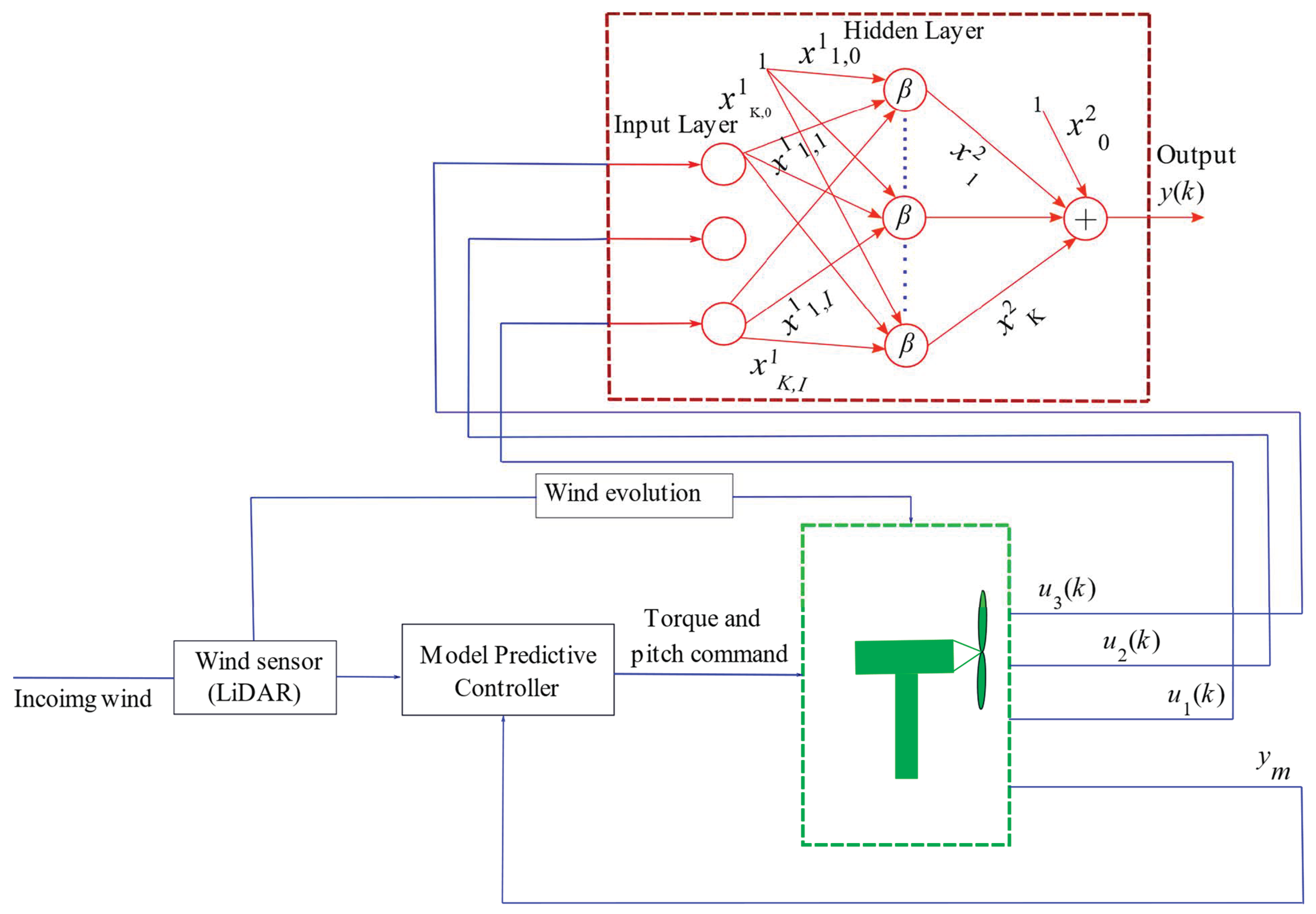
This study uses the double-layer perceptron feedforward structure for pattern recognition to estimate the wind, as shown in Figure 3. Its generalised nonlinear model is mathematically described as follows:

$$y\left(k\right)=h(u_1\left(k\right),u_2\left(k\right),u_3\left(k\right)),$$

(11)

where u₁(k), u₂(k), and u₃(k) are the inputs to NN, y(k) is the output, i.e., wind speed. Furthermore, β is the following bipolar sigmoid activation function:

B(x) = tanh(αx),

(12)

where α is a constant (normally set to 1).

The first-layer weights are represented by $x_{i,j }^1$ where i = 1, 2, …, K, j = 0, 1, …, I, and the second-layer weights are denoted by $x_{i }^2$, where i = 0, 1, …, K. The output is calculated as follows [38]:

$$y\left(k\right)=x_{0 }^2+{\displaystyle {\sum }_{i=1}^K}{x}_{i }^2\beta \left(v_i\left(k\right)\right).$$

(13)

The resultant output of the $ith$ hidden neuron is as follows:

$$v_i\left(\mathrm{k}\right)=x_{i,0}^1+x_{1,1}^{1}u\left(k\right)+x_{2,1}^{1}u\left(k\right)\dots +x_{K,1}^{1}u\left(k\right).$$

(14)

Eventually, the NN is trained by minimizing the following error:

$$\mathrm{e}={\sum }_{i=1}^m{(y\left(k\right)-\tilde{y} \left(k\right))}^2,$$

(15)

where $y\left(k\right)$ and $\tilde{y} \left(k\right)$ denote the measured output and the output estimated by the NN, respectively, and m represents the total number of samples.

The NN utilises the Levenberg–Marquardt (LM) algorithm. As with the quasi-Newton method, LM uses the Jacobian method to calculate the gradient as follows.

$$g=J^{T}e$$

(16)

where J is the Jacobian matrix consisting of the first derivatives of the NN errors regarding the weights and biases, and e is a vector of the NN errors.

Using the backpropagation technique, the Jacobian matrix can be computed by treating the performance function as a mean squared error (MSE). Therefore, the NN trained with the LM algorithm utilises the MSE function to determine the effectiveness of the NN. The wind speed data used to train the NN is acquired from the full nonlinear described in Section 2.

A feedforward NN is constructed for wind speed estimation; the network architecture consists of three layers, each with 20 neurons. The network is trained using three inputs (different combinations of rotor speed, fore-aft acceleration, tower bending moment, and generator torque) and one output (wind speed), each containing 25,000 samples. The training algorithm used is the Levenberg–Marquardt method, which iteratively adjusts the weights and biases of the network to minimize the root mean square error (RMSE) performance function. The activation function is the rectified linear unit (ReLU) [36,37,38,39].

During training, a learning rate of 0.2 is applied, controlling the step size of parameter updates. The training data is divided into batches of size 64, which are processed before updating the parameters of the network. The training process is repeated for 1000 epochs, representing complete iterations over the entire data set. Note that this is still a preliminary study, and in the future, more realistic data, such as field data, will be used instead. In this paper, 70% of the data is used for modeling the NN, 20% of the data is for testing the NN, and the remaining 10% of the data is for validating the NN model with a sampling rate of 100 Hz. The training algorithm, activation function, learning rate, batch size, and a number of epochs are selected to facilitate effective learning and the convergence of the NN. Similar results have been obtained for different wind speeds, although, they are not presented in this paper due to the page limit.

The NN-based estimator is trained and operated as follows:

(1)

Turbine 1 is equipped with a LiDAR, while the remaining turbines are equipped with nonlinear NN-based estimators, as discussed earlier.

(2)

Data required for training the NN-based estimators are collected from turbine 1 at regular intervals, such as every 1000 s. The inputs for training the NN-based estimators consist of a combination of torque, rotor speed, and tower bending moment, and the output for training the NN-based estimators is the wind speed from turbine 1.

(3)

Each of the remaining turbines (turbines 2–5) is equipped with a trained NN-based estimator, providing the turbines with wind speed estimation.

(4)

Steps (2) and (3) are repeated every 1000 s.

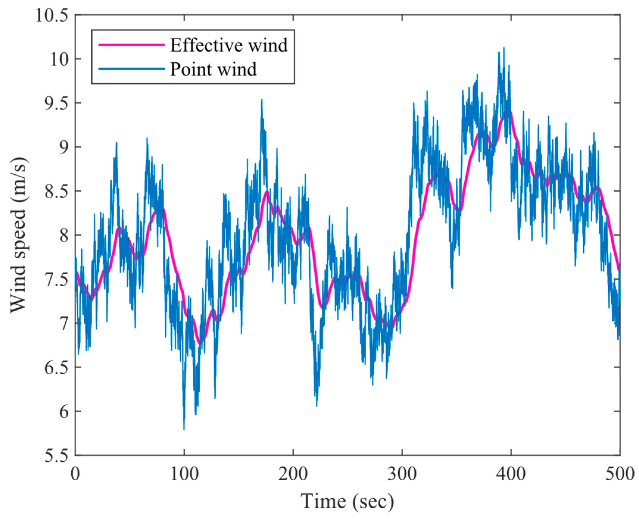
Simulations are carried out in Matlab/SIMULINK. Figure 4a and Figure 5a show the wind speed estimated (in pink) by the NN-based estimator for turbine 2 (randomly chosen) compared with the actual measurement (in blue) at mean wind speeds of 8 and 16 m/s, respectively. It should be noted that the actual measurements (in blue) would not be available in real-world scenarios but are presented here for comparison purposes only.

The time responses demonstrate that the wind estimated by the NN-based estimator attached to turbine 2 tracks the measured wind closely at mean wind speeds of 8 and 16 m/s. The corresponding power spectral densities in the frequency domain are shown in Figure 4b and Figure 5b, respectively. The frequency responses also indicate that the estimation closely matches the measurements.

To investigate whether the differences in the PSDs shown in Figure 4 and Figure 5 amount to significant differences in the time domain, the MSE, RMSE, and mean absolute error (MAE) have also been calculated at two different mean wind speeds, as shown in

Table 1. Performance evaluation metrics for turbine 2.

Metric	At 8 m/s	At 16 m/s
MSE	0.009	0.095
RMSE	0.69	0.75
MAE	0.60	0.70

. The results in the table show that the differences are not very significant.

In summary, the time and frequency responses demonstrate that the wind estimated by the NN-based estimator for turbine 2 closely tracks the measured wind at mean wind speeds of 8 and 16 m/s. Furthermore, similar results have been obtained for different turbines and at different wind speeds, although, they are not included in this paper due to the page limit.

Although the five turbines are assumed to be the same, their interaction may yield complicated wind fields. To guarantee the accuracy and practicality of the NN-based estimator, it should be trained under as various wind conditions as possible, e.g., considering the upstream wind turbines’ wake, etc. However, in this study, it is assumed that the wind turbines are aligned side-by-side, implying that the interaction of the wind field is kept relatively simple. Situations with various kinds of complicated wind fields will be investigated in more detail in future work.

4. Design of Controllers

In this section, the design of controllers (FB and FF-MPCs) for below-rated, rated, and above-rated operations is explained. More precisely, the control objectives and strategy are explained in Section 4.1, and the control syntheses are reported in Section 4.2.

4.1. Control Strategy

The design objectives of the controllers for different operating modes can be described by referencing the control strategy curve in the torque-speed plane illustrated in Figure 6. In Mode 1, the C_pmax curve is followed by regulating the torque demand; in Mode 3, the rated power (5 MW in this case) is maintained by active pitching; Mode 2 can be considered a buffer zone, where the torque is adjusted to track a constant generator speed (120 rad/s in this case).

In more detail, the C_pmax curve in Mode 1 is tracked by minimising the following index:

x₁ = T_e − k.ω²

(17)

where T_e is the generator torque, and k represents a constant that defines the C_pmax curve in Mode 1.

The vertical line in Mode 2 is followed by minimising x₂ given by

x₂ = ω − ω_rated,

(18)

where ω_rated is 120 rad/s in this example.

Through active pitching, the rated power (P_rated) in Mode 3 is maintained by minimising x₃ given by

x₃ = P − P_rated

(19)

where P_rated is the rated power of 5 MW.

4.2. Synthesis of Controllers

FB-MPCs are first designed using the linearised models from Section 2.4. Then, the FB-MPCs are improved by incorporating a feedforward component that utilises the upcoming wind speed information, reported in Section 3, resulting in FF-MPCs. A flowchart justifying the overall controller strategy is shown in Figure 7.

The FB-MPCs are designed using Equation (10) in Section 2, and the FF-MPCs are designed utilising the modified state-space equation below, which includes wind disturbance terms:

$$\begin{gathered} x\left(k+1\right)=Ax\left(k\right)+B_{1}u\left(k\right)+B_{2}w\left(k\right) \\ y\left(k\right)=Cx\left(k\right)+D_{1}u\left(k\right)+D_{2}w\left(k\right) \end{gathered}$$

(20)

where $y\left(k\right)$ is the generator speed, $u\left(k\right)$ is the torque demand in Modes 1 and 2 and pitch demand in Mode 3, and $w\left(k\right)$ is the upcoming wind speed, measured by the LiDAR or estimated by the NN-based estimator reported in Section 3. Note that the last terms ($B_{2}w\left(k\right)$ and $D_{2}w\left(k\right)$) in the state and output equations are only used for the FF-MPCs because they are only concerned with wind information, which is unavailable for the FB-MPCs.

The prediction matrices for the FF-MPCs are as follows:

$$\begin{gathered} \underset{\underrightarrow{y_k}}{\underbrace{\left[\begin{array}{l}{y}_{k+1}\\ y_{k+2}\\ y_{k+3}\\ ⋮\\ y_{k+n_y}\end{array}\right]}}=\underset{S_x}{\underbrace{\left[ \begin{array}{l} C\\ CA\\ C{A}^2\\ ⋮\\ C{A}^{n_y-1}\end{array}\right]}}{x}_k+\underset{Q_u}{\underbrace{\left[\begin{array}{l} D_1 0 \cdots 0\\ C{B}_1 D_1 \dots ⋮\\ CA B_{1}C{B}_1\\ ⋮ ⋮ ⋮ 0\\ C{A}^{n_y-2}{B}_1 C{A}^{n_y-1}{B}_1 \dots D_1\end{array}\right]}}\underrightarrow{u_k} \\ +\underset{T_w}{\underbrace{\left[\begin{array}{l} D_2 0 \cdots 0\\ C{B}_2 D_{2 } \dots ⋮\\ CA{B}_2 C{B}_2\\ ⋮ ⋮ ⋮ 0\\ C{A}^{n_y-2}{B}_2 C{A}^{n_y-1}{B}_2 \dots D_2\end{array}\right]}}\underrightarrow{w_k} \end{gathered}$$

(21)

where S_x, Q_u, and T_w are the prediction matrices. n_y is the prediction horizon and n_h is control horizon.

The D₂ matrix is set to zero and non-zero for the FB-MPCs and FF-MPCs, respectively. The values of $\underrightarrow{u_k}$ and $\underrightarrow{w_k}$ are given by

$$\overrightarrow{u_k}={\left[u_{k+1}{u}_{k+2}\dots u_{k+n_h-1}{u}_{k+n_h}{u}_{k+n_h}\dots u_{k+n_h}\right]}^T$$

(22)

$$\overrightarrow{w_k}={\left[w_{k+1}{w}_{k+2}\dots w_{k+n_h-1}{w}_{k+n_h}{w}_{k+n_h}\dots w_{k+n_h}\right]}^T$$

(23)

The control design is realised by minimising the following cost function $\left(J\right)$ given by

$$J={\sum }_{j=1}^{n_y}{\overrightarrow{e}}_{k+j}{}^T{\overrightarrow{e}}_{k+j}+{\sum }_{j=0}^{n_h}{\overrightarrow{\mathsf{\Delta }u}}_{k+j}{}^T{W}_x{\overrightarrow{\mathsf{\Delta }u}}_{k+j},$$

(24)

where r is the reference, e is the tracking error (the difference between r and y), $W_x$ is the weight matrix, and the control increment is denoted as ∆u.

Using Equations (21) and (24), the $\left(J\right)$, can be written as:

$$J=\left|Lr-S_{x}x\left(k\right)-Q_u{u}_{fut}-T_{w}w\left(k\right)-L\times \sigma \right|+W_x \left|u_{fut}\right|,$$

(25)

where L signifies the vector of ones and its size is n_y$\times 1$, and the weight matrix is denoted as $W_x$. The symbol $\sigma$ is the offset, the difference between the output of the process and the model.

Equation (25) is deduced as the control input function,

$$J\left(u,k\right)=u_{fut}{}^T \underset{N}{\underbrace{\left( Q_u{}^{T } Q_u+W_x\right)}}\times u_{fut }+2 u_{fut}{}^T\times \underset{P}{\lceil \underbrace{\begin{array}{c}\left((Q_u{}^{T }{S}_x)\times x\left(k\right) \right)-\left((Q_u{}^{T } L+W_x M)\times \left(r-\sigma \right)\right)+\\ \left((Q_u{}^{T }{T}_w)\times w\left(k\right) \right)\end{array}}\rceil }$$

(26)

where M = ($u_{ss}/(r-\sigma$)) is steady state input gain.

Finally, the derived constraint quadratic cost function is as follows:

$$minJ\left(u,k\right)=u_{fut}{(k)}^{T}N{u}_{fut}\left(k\right)+u_{fut}{(k)}^{T}P,$$

(27)

and it is subject to the following constraints of

$$\begin{gathered} u_{min}\le u_{fut}\le u_{max} \\ \Delta u_{min}\le \Delta u_{fut}\le \Delta u_{max} \\ y{\left(k+1\right)}_{min}\le y\left(k+1\right)\le y{\left(k+1\right)}_{max}, \end{gathered}$$

(28)

where u_min and u_max are the lower and upper limits of u_fut, respectively. The symbols ∆u_min and ∆u_max are the lower and the upper limits of ∆u_fut, respectively.

5. Simulation Studies

The FB and FF-MPCs designed in Section 4 are evaluated using the full nonlinear model described in Section 2 to test their control performance, including their robustness to the model–plant mismatch. In this paper, the FB-MPCs are applied to the more sophisticated full nonlinear model to test the design’s robustness to some degree. Simulations are conducted in both the frequency and time domains to evaluate the controllers’ performance in the torque-speed plane, with and without wind estimation. Furthermore, the controllers are compared with the conventional PI controllers and also FF-PIs.

5.1. At Below-Rated Wind Speed

In this section, the FB and FF-MPCs are tested in both the time and frequency domains at a below-rated wind speed with a turbulence intensity of around 15% (per IEC class C standards) [48]. The prediction horizon, n_y and control horizon, n_h, are taken as 20 and 15, respectively, with a weight of 2 × 10⁻¹². The sampling time (T_s) is set to 0.02 s.

Figure 8 compares the generator speeds (measured output) produced by the FB and FF−MPCs at a below-rated wind speed (i.e., at a mean wind speed of 8 m/s). However, from these plots, it is very hard to assess the performance of tracking the C_pmax curve, which is the main control objective in Mode 1, as previously mentioned. In Mode 1, the wind turbine’s low wind-speed operating region, the control objective is to harness the maximum power possible from the wind—this is achieved by tracking the C_pmax curve in the torque/speed plane shown in Figure 9, for instance. 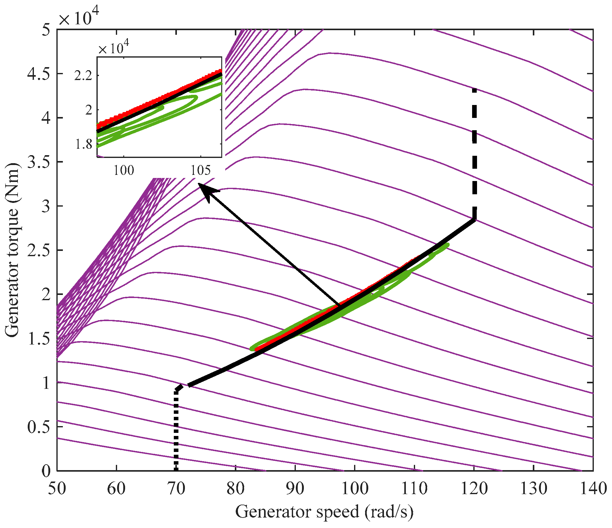Hence, the performance of the controllers is tested in the torque/speed plane, as portrayed in Figure 9.

Figure 9 shows that the FF-MPC tracks the C_pmax curve more accurately than FB-MPC because the C_pmax curve, the black line, is followed more tightly by the red plots (FF-MPC) than the green plots (FB-MPC). This is due to the controller’s feedforward component obtained mainly through NN-based estimation.

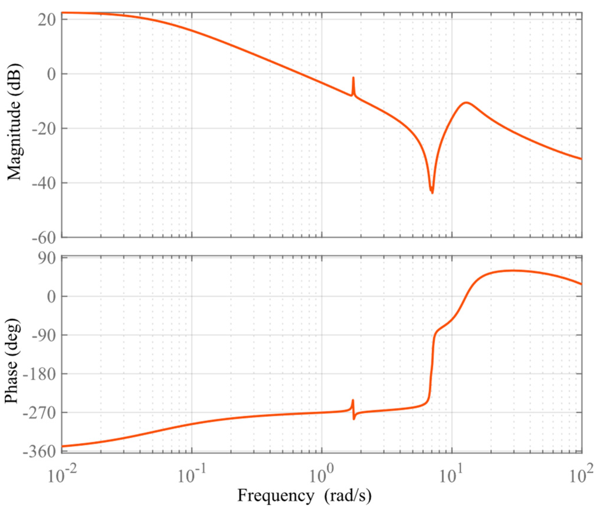
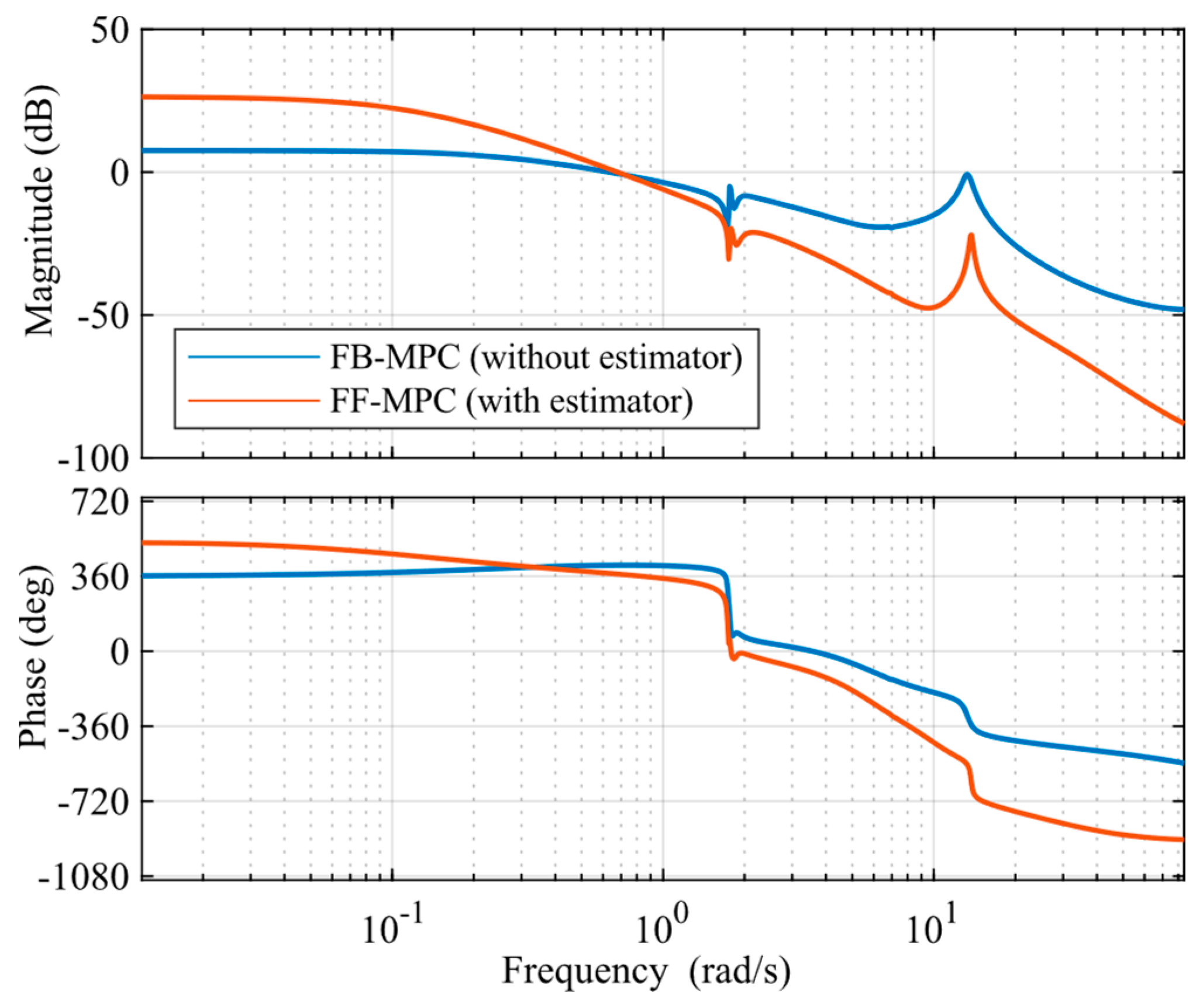
Figure 10 illustrates the control performance in the frequency domain. The gain crossover frequency (GCF) should be between 0.6 and 2 rad/s [49]. A GCF below 0.6 rad/s can lead to a sluggish control, while a GCF above 2 rad/s can result in an overly aggressive control.

From the above findings, it can be concluded that an improved time response and more precise C_pmax tracking on the torque/speed plane, which would lead to improved power efficiency, are accomplished when wind estimation is incorporated (compared to the FB-MPC without wind estimation). Notably, the GCF of the controller (FF-MPC), as shown in Figure 10, fell within the acceptable range, and this improvement is achieved without increasing control activity with the use of FF-MPC.

It can also be observed that the peak around 10 rad/s is below 0 dB. This is another significant finding, as conventional PI controllers necessitate a drive-train damper to ensure these peaks do not crossover 0 dB [50].

A quantitative evaluation is made in Mode 1, as given in

Table 2. Controller performance in each mode.

Parameters	FB-MPC without Estimator	FF-MPC with Estimator
Mean power efficiency in Mode 1	98.40	99.21
RMSE of generator speed in Mode 2	5.42	3.56
RMSE of power in Mode 3	1.9410 × 105	1.7709 × 104

RMSE: Root mean square error.

(second row). The comparison in the table shows that the improved mean power efficiency is achieved by FF-MPC in Mode 1, confirming what has been discussed in this section; that is, FF-MPC outperforms FB-MPC in Mode 1. Table 2 and Figure 9 demonstrate moderate improvement, i.e., 0.8% is achieved. As discussed later in the section, improvement is expected to be more significant at higher wind speeds.

5.2. At Just Above-Rated Wind Speed

This section demonstrates the responses of the FF-MPC and FB-MPC at a mean wind speed of 12 m/s. Figure 11a depicts the measured output (i.e., generator speed), and the corresponding control inputs, i.e., pitch angles, with and without the wind estimator, are shown in Figure 11b. The results demonstrate that the improvement in control performance is attained due to phase lead in control input (pitch angle) rather than increased pitch activity, as depicted in Figure 11b.

A quantitative evaluation is also made in Mode 2, as given in Table 2 (third row). The comparison shows that FF-MPC achieves improved RMSE of generator speed compared to the FB-MPC.

5.3. At Above-Rated Wind Speed

This section tests the FB and FF-MPCs in the time and frequency domains for a mean wind speed of 16 m/s. The n_y, n_h, and weight are set to 20, 10, and 3 × 10⁻¹⁰, respectively. To maintain the rated wind speed of the 5 MW machine, the generator speed is maintained close to 120 rad/s, as explained in Section 4.1.

The results in Figure 12a illustrate that the FB-MPC (in blue) maintains the generator speed close to 120 rad/s very well, keeping fluctuations given in Equation (29) below 12%, which usually is a requirement [50]. However, the figures also illustrate that the FF-MPC yields improved results compared to the FB-MPC, as expected.

$$N=\left(\left(y_{max}-y_{mean}\right)/y_{mean}\right)$$

(29)

The corresponding control inputs (pitch angles) for both controllers are shown in Figure 13. The comparison reveals that the improvement observed in Figure 12 is not owing to more aggressive control but rather to a phase lead in the control input. The incorporated wind speed estimation let the FF-MPC react to the variations in the approaching wind earlier than FB-MPC, significantly improving power fluctuations, as shown in Figure 12b, without increasing the control action.

The similarity between the GCFs of the two controllers is evident, as shown in Figure 14. This indicates that the aggressiveness of the FB-MPC is nearly identical to that of FF-MPC. Furthermore, the GCF of both controllers is within the satisfactory range, as shown in Figure 14. Importantly, the peaks at around 11 rad/s remained below 0 dB for both controllers, which is another important finding since traditional PI-based controllers require a drive-train damper to maintain the peaks below 0 dB [50].

To attain robustness, the controller should produce an acceptable GCF between 0.6–2 rad/s [49]. A GCF below 0.6 rad/s can create a prolonged control action, whereas a GCF greater than 2 rad/s can cause an excessively aggressive action. For better understanding, simulations are conducted on a 5 MW Supergen exemplar wind turbine at 16 m/s mean wind speed. The robustness of the controller is confirmed by simulating it with different design parameters. The n_y, n_h, and weighting factors are varied to observe their impact on the frequency response of the controller. Figure 15 demonstrates that the GCFs (directly related to the bandwidth) are within acceptable limits, confirming that the controller’s robustness remains intact without increased aggressiveness, which is remarkable.

For case: 1 (GCF at 1.02 rad/s), n_y, n_h, and weight are taken as 20, 10, and 2 $\times$ 10⁻¹⁰, respectively; for case: 2 (GCF at 1.13 rad/s), n_y, n_h, and weight are 15, 10, and 2 $\times$ 10⁻¹², respectively; and for case: 3 (GCF at 1.2 rad/s), n_y, n_h, and weight are 25, 15, and 3 $\times$ 10⁻¹⁰, respectively.

The weighting factor needs to be chosen suitably, and there exists a tradeoff among parameter selections, such as n_y, n_h, and sampling time, which affect the responses of the turbines in the time and frequency domains.

A quantitative evaluation is also made in Mode 3, as shown in Table 2 (bottom row). The result indicates that the FF-MPC outperforms the FB-MPC in Mode 3, with a reduced RMSE, which is consistent with the findings discussed in this section.

5.4. Comparison with Standard Controllers

The comparison between the FF-MPC and conventional PI-based controllers is discussed in this section. First, simulation results are presented for the PI, FF-PI, and FF-MPC together. Then, the corresponding outputs (generator speed) at a mean wind speed of 16 m/s are displayed in Figure 16a. The results indicate that the FF-MPC significantly reduced the generator speed fluctuations compared to the PI and FF-PI.

Figure 16b displays the demanded pitch angles for the PI, FF-PI, and FF-MPC to demonstrate that the FF-MPC achieves improved control due to a phase advance in pitch angle rather than increased pitch activity compared to the PI and FF-PI.

The corresponding open-loop frequency responses are shown in Figure 17. GCFs are within the acceptable range, between 0.6 to 2 rad/s, which shows that all the controllers are neither too aggressive nor unresponsive. However, the PI and FF-PI show peaks exceeding 0 dB at about 13.5 rad/s, which would require a drive-train damper to keep them below 0 dB [50]. By contrast, the FF-MPC and FB-MPC do not need a drive-train damper, which is a significant advantage.

5.5. Discussion

In summary, the time (generator speed and pitch demand) and frequency responses and the table in this section demonstrate that the FF-MPC outperforms the PI, FF-PI, and FB-MPC, as expected. Improvements are much more significant in above-rated wind speeds than in the below-rated wind speed. Importantly, the improvement is not due to increased control activity but to a phase lead enabled by LiDAR and wind estimation. The model–plant mismatch between the control design model, based on which the controllers are designed and the more sophisticated full nonlinear model, to which the designed controllers are applied, let the controllers’ robustness be assessed to some extent. This study assumes that the wind measurement is perfect, implying that wind evolution [42,43] can be neglected. Based on this assumption, the wind speed is estimated using the NN-estimator discussed in Section 3. If the wind evolution is included, the results are expected to deteriorate. Likewise, when the controllers are applied to a high-fidelity aeroelastic model or the real-life turbine of the exemplar turbine, the control performance is also expected to degrade.

6. Conclusions and Future Work

This study presents the application of the MPCs to a full nonlinear 5 MW Matlab/SIMULINK model of the same exemplar Supergen wind turbine using NN-based wind speed estimation. In this work, first, the FB-MPC controller is designed using linearised models derived from the full nonlinear model of the Supergen 5 MW turbine. In addition, the control performance is improved by incorporating a feedforward component that uses the upcoming wind speed information obtained through a NN-based estimation as part of the controller design, yielding the FF-MPC.

To make the system economically feasible, a LiDAR is shared in a cluster of several wind turbines (five in this paper). In more detail, one of the five turbines is equipped with only LiDAR, and each of the remaining four turbines with a NN-based estimator, which in effect replaces the LiDAR for other turbines, reducing the overall cost significantly.

Both the FB and FF-MPC, designed based on the linearised models, are applied to a much more detailed full nonlinear model to test the robustness of the controller design. Simulations are conducted at varying wind speeds, and the controllers are thoroughly evaluated in the frequency and time domains, as well as in the speed-torque plane. As expected, the simulation results demonstrate that the FF-MPC performs better than the FB-MPC without increasing the pitch activity of the turbine; that is, the controller’s bandwidth (or the GCF) remains within the acceptable range. The FF-MPC is also tested against conventional PI and FF-PI controllers. The results illustrate that the FF-MPC also outperforms both controllers. Another notable finding is that the FB and FF-MPC do not require a drive-train damper, which sets them apart from conventional PI-based controllers.

In future work, the controllers will be applied to a high-fidelity aeroelastic model of the same turbine, i.e., the DNV-Bladed or NREL FAST model. Additionally, wind evolution from the LiDAR to the rotor, not considered in this study, will be examined by applying the controllers to a high-fidelity aeroelastic model that takes into account the effect of wind evolution.